Abstract
All long-term hydropower planning problems require a forecast of the inflow during the planning period. However, it is challenging to accurately forecast inflows for a year or more. Therefore, it is common to use stochastic models considering the uncertainties of the inflow. This paper compares deterministic and stochastic models in a weekly rolling horizon framework considering inflow uncertainty. The stochastic model is tested in both a risk-neutral and a risk-averse version. The rolling horizon framework helps make periodic decisions and update the information in each rolling week, which minimizes the errors in prolonged forecasts. The models aim to utilize the water stored in the rainy season throughout the year with minimum load shedding while storing as much water as possible at the end of the planning horizon. The Conditional Value at Risk () risk measure is used to develop the risk-averse stochastic model. Three different risk measures are investigated to choose the risk measure that yields the best outcome in the risk-averse problem, and the two best measures are compared to a deterministic and risk-neutral model in a weekly rolling horizon framework. The results show that the risk-neutral and best risk-averse models perform almost equally and are better than the deterministic model. Hence, using a stochastic model would be an improvement to the actual planning performed in the Ethiopian and other African countries’ power systems.
1. Introduction
Many hydropower plants have large reservoirs, which allow water to be stored for an extended period of time. This water is used when the demand is high or other generation sources are scarce in the system. In many cases, there are a few short periods with substantial inflow each year. The task of long-term hydropower planning is to decide during which periods this water should be used. In a country like Ethiopia, where hydropower plants dominate power generation, the challenge is to decide how to use the inflow from the rainy season while considering the uncertainty of future inflow. Hydropower planning will, therefore, have to find an appropriate trade-off between using the available water now (risking future energy shortages) or starting load shedding to a smaller extent now. Therefore, all long-term planning problems require a forecast of the inflow during the planning period. However, it is challenging to accurately forecast the inflow to hydropower reservoirs with a reasonable time resolution (preferably not longer than one week) for one year or more. Therefore, it is common to use stochastic planning models, where the planning is based on several possible scenarios.
For a vertically integrated electricity market dominated by hydropower plants, where the government determines the electricity prices without any competition, like in Ethiopia and most African countries, there is no price uncertainty, but the most crucial factor in proper hydropower scheduling is the uncertain inflow. A straightforward solution to such scenarios is to use historical data, i.e., to assume that the inflow during the year will be similar to what was recorded in earlier years. Alternatively, one of the methods presented in [1] can be employed for scenario generation through selection from historical data, using techniques such as sampling, k-means clustering, and scenario reduction methods, provided that sufficient historical inflow datasets are available. If a sufficient dataset of historical inflow data is unavailable and there is a lack of accurate measurements (as in the case of Ethiopia and many African countries), another method is needed to generate inflow scenarios. Here, we use the methods described in [2]. In this paper, a method to generate inflow data is developed based on the correlation between generation statistics in the Ethiopian power system and publicly available precipitation statistics in the specific locations of the reservoirs.
Hydropower planning models have been developed over the past few decades [3,4,5,6]. There are various ways to model hydropower for the short term and long term, including deterministic [7,8,9,10,11] and stochastic models [12,13,14,15], as well as risk-neutral and risk-averse models [16,17,18]. Moreover, the rolling horizon framework has long been used to solve stochastic programming models in different applications. For instance, a rolling horizon framework was used in [19,20,21,22,23,24] for unit commitment problems, production decisions, load shedding strategies, and so on.
In general, hydropower planning models minimize operation costs or maximize profits using different levels of detail and mathematical formulations. Thus, there is a wide variety of possible models for hydropower planning to choose from. The challenge is to find a model that yields good results in an Ethiopian context, where the primary goal of planning is to supply uninterrupted power to end users and utilize the water in the rainy season throughout the year with minimal load shedding. However, load shedding during the planning period has to be weighed against the risk of large load shedding in the future if not enough water is stored in the reservoirs at the end of the planning period.
The objective of this paper is to test how efficient some of the long-term planning models would be in the Ethiopian system due to its special characteristics, i.e., a hydro-dominated system dependent on seasonal rainfall. The reservoirs receive most of their inflow during the short rainy season; therefore, there is a need to determine how to allocate the water over the coming year. Another challenge in the system is the lack of availability of organized data. The other objective is to identify which models are best at avoiding load shedding in the system.
The contribution of this paper is, therefore, to develop a long-term stochastic hydropower planning model for the Ethiopian power system considering uncertain inflows. The aim of the planning model is to minimize or avoid load shedding occurring in the dry season in the system by optimizing the scheduling of the hydropower plants in such a way that excess water in the rainy season is stored and utilized in the dry season. It is computationally difficult to plan a stochastic model in the long term, as the time step is smaller and the number of scenarios is larger. In addition, it is difficult to obtain an accurate forecast for long-term planning. Forecast information should be updated intermittently throughout the planning horizon. Therefore, the other contribution of this paper is to test the planning tools in a rolling horizon framework for the long-term stochastic model, in which only a subset of the time horizon decisions is considered at a time. The model rolls in a fixed horizon, with the first period updated in each roll.
According to the information collected from Ethiopian Electric Power (EEP) and as discussed in [2], generation and operation planning in the Ethiopian power system is fully dependent on the relationship between the historical generation and historical water level patterns of the reservoirs. There is no planning tool developed so far to consider uncertain environmental incidents. Therefore, this long-term stochastic model could be used as a substitute for traditional planning methods based on historical data.
2. Mathematical Model
2.1. Problem Definition
A long-term stochastic model is developed for the Ethiopian power system considering the existing large hydropower plants that were functional in the 2018–2019 planning year [25]. The generation from three wind power plants and a waste-to-energy plant is taken as a constant value from historical generation data. Details of the Ethiopian hydropower system are provided in [2]. The stochastic model is developed in a weekly time step for a one-year planning horizon considering uncertain inflow scenarios to the reservoirs. The inflow scenarios are generated using the method described in [2]. The data on the weekly load demand for the 2018–2019 planning year and the contents of the reservoirs at the start of the planning year are collected from EEP. The value of stored water is calculated from the future electricity price and the amount of energy that could be generated from the stored water. A penalty cost is taken into account for load shedding.
2.2. Assumptions
One of the biggest challenges in the Ethiopian and most African countries’ power systems is the availability of well-organized data. To overcome this challenge, we have made some reasonable assumptions in the model development process.
The model neglects the head dependency of the hydropower plants and the efficiency curve of the turbines; therefore, generation is approximated as a product of the discharge () and production equivalent () of the power plant (). The starting contents of the reservoirs () are assumed to be the average of the starting contents for the past ten years. The minimum discharge () from all the reservoirs is assumed to be zero, except for reservoirs with downstream sugar cane plantations. The water delay time between cascaded hydropower plants is neglected. The system is considered as one area, i.e., transmission limitation is neglected, and power export to neighboring countries is considered from historical data.
2.3. Stochastic Optimization Model
The stochastic optimization model maximizes the value of stored water and minimizes load shedding, considering the uncertainties in the inflows of the reservoirs. The optimization problem is realized as a two-stage stochastic model with a weekly time resolution and a one-year planning period. The first stage comprises the first week of the planning period, and the second stage comprises the rest of the year and all inflow scenarios, as shown in the scenario tree in Figure 1.
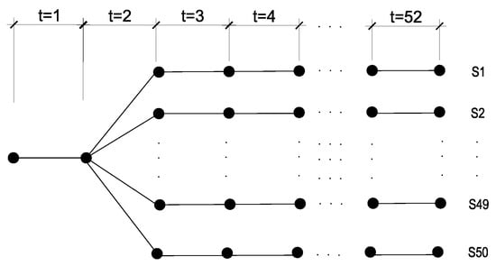
Figure 1.
Scenario tree.
2.3.1. Objective Function
The objective function consists of two sub-functions. The first function maximizes the value of the stored water (1), and the second function minimizes the penalty cost of load shedding (2).
Therefore, the overall objective function maximizes the difference between the value of stored water () and the cost of load shedding (). The first constraint is the hydrological balance (5), i.e., the reservoir contents at time t equal the sum of all the inflows minus the sum of all the outflows at the same time t. The next constraint is the load balance constraint (6), i.e., the total generation from all power plants should satisfy the local demand plus the export. If the demand exceeds the generation, the excess load will be the load shedding. Finally, there are different variable limits, as described in Equations (8)–(12). The non-anticipativity constraint for the first stage of the stochastic model (13), which describes the discharge at time t, is not scenario-dependent for the first stage.
2.3.2. Risk Measures
Risk measures are used to characterize the risk associated with a given decision. The main advantage of considering risk measures is that it is possible to avoid the very low costs experienced in some unfavorable scenarios in profit maximization. A risk measure can be incorporated either into the objective function of the problem or as an additional set of constraints in the problem formulation [26].
In this paper, we consider two types of risk. The first is the load shedding risk, which is concerned with the occurrence of unnecessary load shedding in the process of water value maximization. This is included in the objective function as a penalty cost of load shedding weighted by a cost factor .
The second is the risk of having empty reservoirs or low reservoir contents at the end of the planning period while minimizing load shedding penalty costs. In order to avoid this risk, we introduce a variable bound for the final contents of the reservoir.
For an equiprobable scenario and a given confidence level , the Conditional Value at Risk () is defined as the expected profit in the worst scenarios [26].
The variable represents the highest profit in the () worst scenario such that the probability of experiencing a profit less than is less than or equal to () [27]. The risk measure is included in the objective function weighted by a risk factor . Therefore, the overall risk-averse equation becomes:
This objective function is subject to the same constraints as the risk-neutral problem (5)–(13). In addition, a risk measure constraint must be added. In this paper, we investigate three possible formulations: three different risk measure constraints.
The risk measure could be considered to account for the risk of low stored water (19a) and high load shedding (19b) separately or in combination, i.e., when the risk measure is considered for the entire objective function (19c). It should be noted that only one of the constraints from (19a) to (19c) should be applied at the same time. The consequences of choosing different risk measure constraints are analyzed in Section 3.2.
2.4. Stochastic Model in a Weekly Rolling Horizon Framework
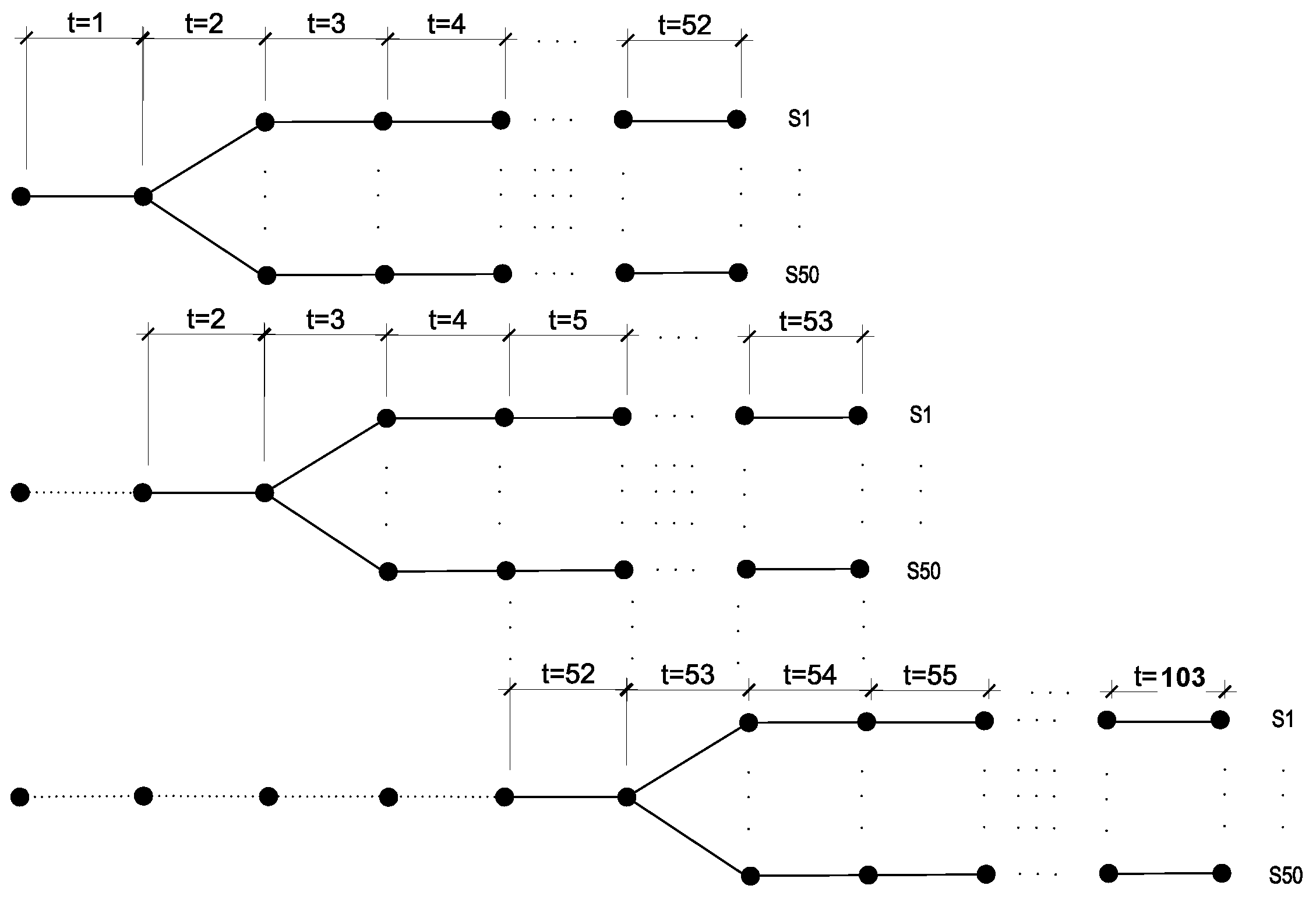
A rolling horizon framework is developed to simulate the two-stage stochastic model described in the previous section. The stochastic model is simulated in a weekly rolling horizon, as shown in Figure 2.
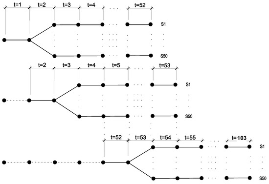
Figure 2.
Scenario tree in a weekly rolling horizon.
The first week’s (week r) operation is based on the stochastic model’s output for the period (), where r is the rolling time step (one week in this case) and T is the planning horizon (one year or 52 weeks in this case). For the first week, the system is operated to generate the sum of the total power scheduled in each plant. This helps in allocating the power scheduled for the run-off of the rivers during the model simulation in case there is insufficient inflow during actual operation. At the end of the week, all the information, such as the inflow, reservoir contents at the end of the week, load shedding, and spillage, is updated and recorded. Then, the model is simulated for the next period () using the updated information. This continues rolling until the end of the planning period (), which is one year in this case.
The algorithms for the risk-neutral (Algorithm 1) and risk-averse stochastic rolling horizon models (Algorithm 2) are described as follows.
| Algorithm 1 Risk-neutral stochastic rolling horizon model |
|
| Algorithm 2 Risk-averse stochastic rolling horizon model |
|
The information about the inflow is updated for the actual inflow of in the rolling week. (21) is used to set the total generation for the rolling week to be equal to the scheduled total generation for the week. At the end of the week, we will know the actual reservoir contents, which are used as the starting contents for the next rolling week. Finally, (22) is the non-anticipativity constraint for the stochastic model of the next rolling horizon.
The problem is analyzed using the JULIA scientific programming tool version 1.7.2, with JuMP mathematical optimizer of version 0.22.3 and Gurobi solver version 0.10.3.
3. Results and Discussion
3.1. Risk-Neutral Model
This section discusses the advantages of considering uncertainties in the planning model to account for unfavorable conditions instead of planning considering average values, i.e., the advantage of using stochastic models over deterministic models. The risk-neutral stochastic model for the first week of the rolling horizon is compared to the deterministic model developed in [25]. The load demand of the 2018–2019 planning year is used for both models. The 50 inflow scenarios in [2] are used in the stochastic simulation. The inflow in the deterministic model is set to be the average of these 50 scenarios.
The Value of the Stochastic Solution () quality metric determines the benefits of solving the stochastic model over the deterministic model. The is the value of the difference between the results of using the expected value solution () and the recourse problem solution () [28]. The compares the profitability of decisions based on uncertainties to those based on the expected value. For a two-stage maximization stochastic problem, the can be calculated as:
where is the optimal value of the stochastic problem (recourse problem), and is the optimal value of the stochastic problem when the first-stage variables are fixed to the values provided by a deterministic problem using expected values for all uncertain parameters.
Table 1 shows the optimal values for the stochastic problem (), , and for the different load level increases in the first week of the rolling horizon model. For the maximization problem, all the values of the for the different load level increases are positive. This indicates that solving the stochastic model is more profitable compared to the deterministic one, and it is worth considering the uncertainties in the inflow in the hydropower planning model.

Table 1.
Value of stochastic solution () for different load level increases in the first week of the rolling horizon.
3.2. Risk-Averse Model
The risk-averse model considers risk measures related to low reservoir contents, high load shedding, and a combination of the two, i.e., the risk of low optimal value in some unfavorable inflow scenarios.
The risk of high load shedding is controlled by varying the penalty cost of load shedding in the risk-neutral problem, which protects the model from high load shedding in the process of stored water maximization. To determine a reasonable penalty cost, the model is simulated for different values of C, as shown in Table 2.

Table 2.
Sensitivity analysis of the cost of load shedding
In the optimization process, a reasonable value is assigned to the value of stored water based on the tariff set in the Ethiopian power system, which is 50 USD/MWh. We simulate the model using different values of the penalty cost to determine how high we should set the penalty cost in the model. As can be seen in Table 2, the load shedding is higher for USD 200, but it is the same for USD 500, USD 750, and USD 1000; hence, regardless of how high the penalty cost is, the system cannot keep the load shedding below 0.65 TWh. Therefore, the highest penalty cost that could be assigned in this model is USD 500.
We use the risk measure in three different cases using Equations (19a)–(19c) to determine the risk measure with reasonable results: Case-a, where the risk measure considers only the value of stored water (constraint (19a)); Case-b, where the risk measure considers only the load shedding (constraint (19b)); and Case-c, where the risk measure considers all the objective functions (constraint (19c)).
The model is simulated for different values. The simulation results presented in Table 3 show that when , the problem is risk-neutral; the values are consistent across all three cases. However, when the value of deviates from zero, the model becomes risk-averse, leading to different results for the different cases.

Table 3.
Summary of risk measure with and different values of .
In Case-a, where the risk measure considers the value of stored water only, as the value of increases from zero to 0.5, the energy in stored water increases by 0.07 TWh and load shedding increases by 0.03 TWh. This is an indication that water is used more efficiently since the increase in stored energy is larger than the increase in load shedding. When comparing to , we can see that the energy in stored water increases by 0.94 TWh and load shedding increases by 0.39 TWh, which, again, means that we store more water in the future at the expense of a small amount of load shedding now. However, further increasing the value of results in a significant amount of load shedding, leading to a very high penalty cost without an equivalent increase in the stored water, which indicates inefficient water use.
In Case-b, where the risk measure considers load shedding only, as the value of increases to 0.5 and 0.75, there are no changes in any of the values; the changes start when , i.e., when we are 100% risk-conscious, at which point, the energy in stored water decreases by 0.65 TWh and load shedding increases by 0.20 TWh, which is less efficient than what we saw in Case-a when .
In Case-c, where the risk measure considers the entire objective function, as the value of increases to 0.5 and 0.75, there are no changes in any of the values; when , the energy in stored water decreases by 1.87 TWh and load shedding increases by 0.57 TWh, which is less efficient than Case-b when and Case-a when .
3.3. Rolling Horizon Model
The results from a single week can only provide an indication as to how well different risk-averse models will perform. Therefore, the different models are evaluated in a weekly rolling horizon framework. This framework allows for making immediate decisions for one week at a time and updating the actual information after each week. The update can also include an updated forecast for the remaining time horizon. However, in this study, we use the same 50 inflow scenarios for the rolling horizon.
The simulation results of the two risk-averse stochastic models are compared to those of the risk-neutral stochastic model and the deterministic model developed in [25]. Based on the results in Section 3.2, the risk-averse model is tested for two risk measures: Case-a with and Case-b with .
The objective of the comparison is to study how they manage load shedding when there is not enough hydropower generation available. In particular, the challenge is the trade-off between load shedding now and in the future. In principle, we can avoid load shedding using all the water we have right now, but then if we have a poor rainy season with low inflow next year, we may face a problem in supplying the demand next year. Therefore, we have to have some margins left if things become worse in the future. This is a challenge for power system planners; they want to avoid massive load shedding events where they have to disconnect almost half the power system. This inevitably disconnects essential loads, leading to enormous problems for society, whereas if we have smaller load shedding, we can implement rotating load curtailments that affect residential areas, which may have a smaller societal impact. Hence, if load shedding is inevitable, it is preferable to have small levels of load shedding for longer periods rather than massive load shedding for shorter periods. The overall objective is still to minimize load shedding as much as possible. Consequently, there are three questions to evaluate for the different planning models:
- What is the total load shedding during a year?
- How much water is saved for the future?
- How is load shedding distributed throughout the year?
The four models are studied as four cases, with the deterministic model considered as Case-D, the risk-neutral stochastic model considered as Case-RN, the risk-averse model with the risk measure of stored water when considered as Case-RA-1, and the risk-averse model with the risk measure of load shedding when considered as Case-RA-2.
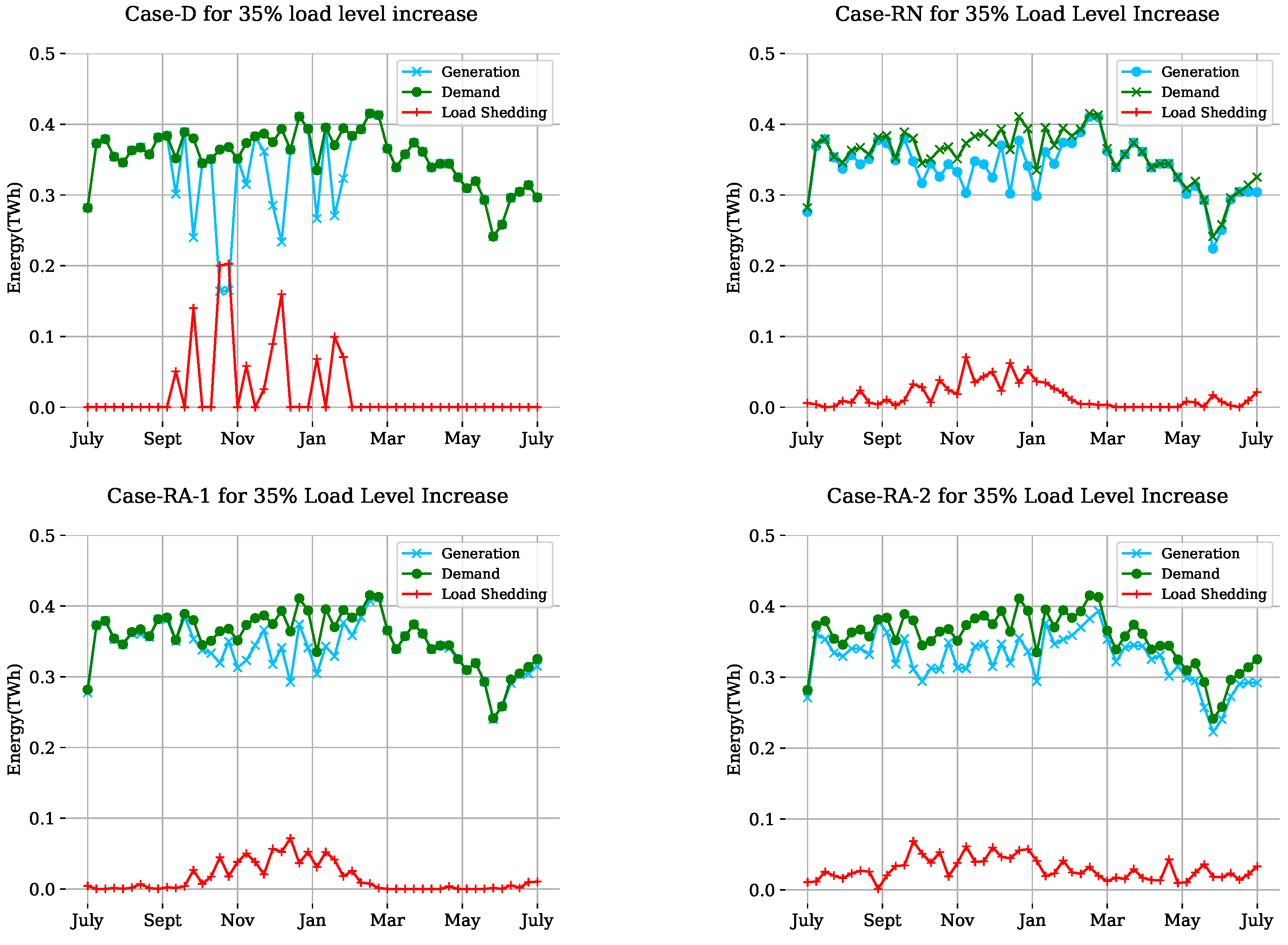
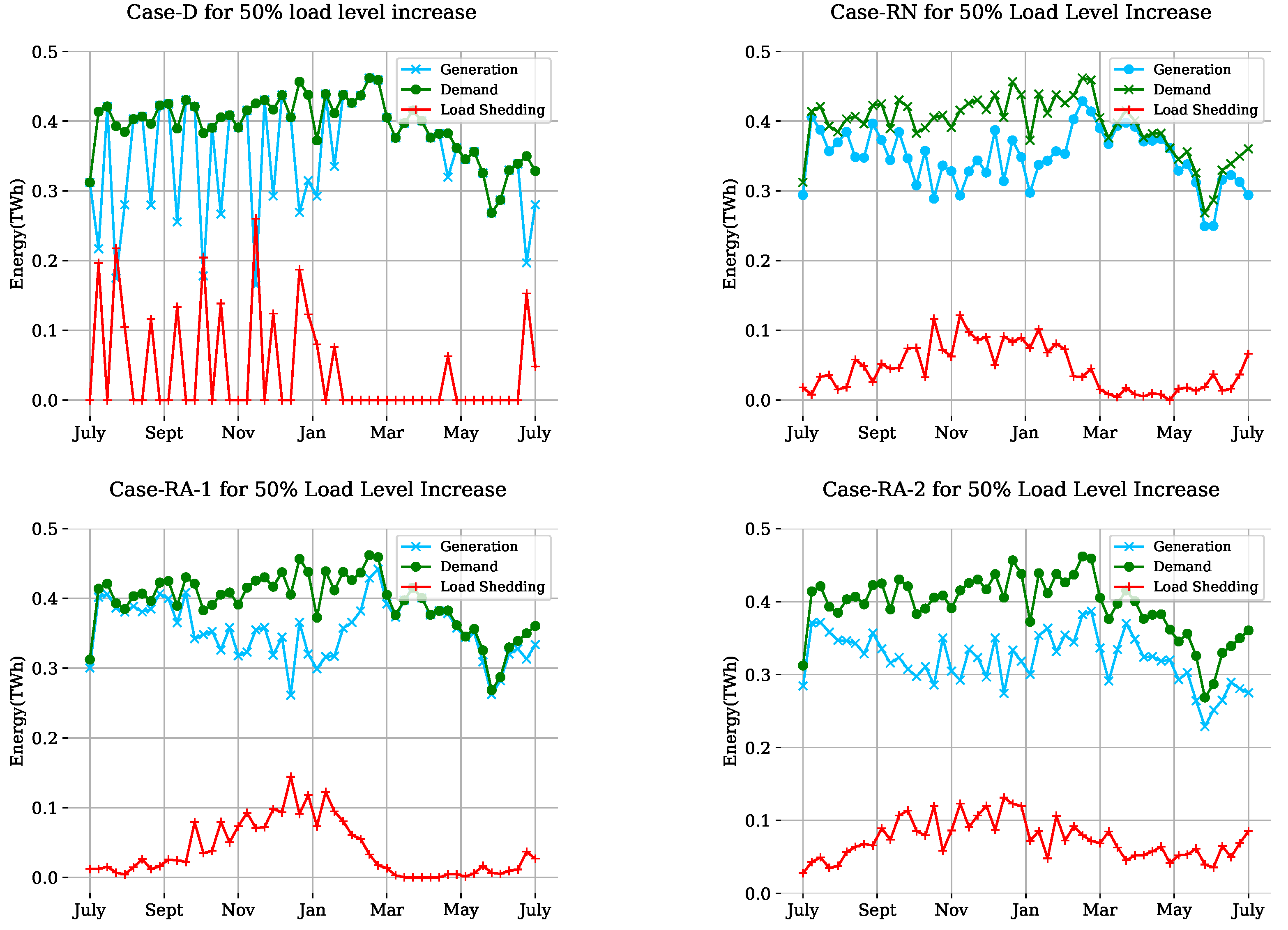
All the cases are simulated in a weekly rolling horizon framework using the synthetic historical inflow from 2018–2019 as the actual inflow to update the information after each one-week time step. The load demand from the 2018–2019 planning year is used as the current load demand. The system supplies the current load demand with zero load shedding in all the cases. Therefore, it would be interesting to see how the system performs in the four cases as the demand increases without additional capacity. All the cases are simulated with load level increases of 35% and 50% from the current load to study the performance when the hydropower capacity is insufficient. The results are summarized in Table 4 and Figure 3 and Figure 4. The two figures show different patterns and distributions of the load shedding throughout the year for the different cases.

Table 4.
Summary of total and maximum load shedding and energy in stored and spilled water in (TWh) for the four cases.
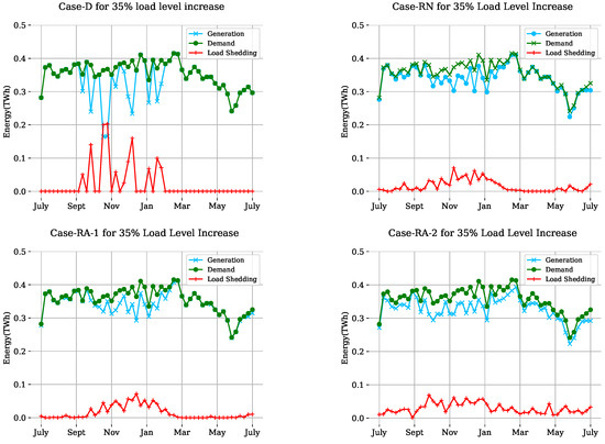
Figure 3.
Generation, demand, and load shedding for a 35% load level increase for the four cases.
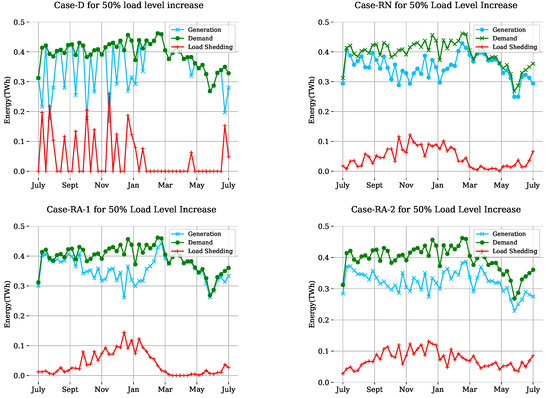
Figure 4.
Generation, demand, and load shedding for a 50% load level increase for the four cases.
For the deterministic model (Case-D), Table 4 and Figure 3 show that for a 35% load level increase, load shedding is concentrated in the second half of the year, totaling 1.17 TWh with a maximum of 0.20 TWh. When the load demand increases by 50%, as shown in Figure 4, we can see frequent, massive load shedding periods starting from the beginning of the planning year and extending to January, totaling 2.23 TWh with a maximum of 0.26 TWh recorded at one time. Moreover, the model stores the least amount of energy for both 35% and 50% load level increases and spills the highest amount of energy for a 35% load level increase. Therefore, Case-D performs poorly based on all the three criteria described.
The risk-neutral stochastic model (Case-RN) evenly distributes load shedding throughout the year, totaling 0.82 TWh with a maximum of 0.07 TWh recorded at one time for a 35% load level increase. The risk-neutral model performs better than the deterministic model regarding total and maximum load shedding, as well as the amount of stored energy. As the load level increases by 50%, as shown in Figure 4, total load shedding becomes higher than that in Case-D and Case-RA-1, but the model distributes load shedding more evenly throughout the year, keeping the value below 0.12 TWh. In terms of stored energy, the model falls between the two risk-averse models; it stores 0.02 TWh more energy than Case-D, 0.07 TWh more energy than Case-RA-1, and 0.20 TWh less energy than Case-RA-2. It spills 0.11 TWh more energy than Case-D, 0.02 TWh more energy than Case-RA-1, and 0.04TWh less energy than Case-RA.
For a 35% load increase, the first risk-averse stochastic model (Case-RA-1) keeps load shedding below 0.07 TWh, the same as Case-RN, throughout the year, totaling 0.77 TWh, which is lower than all the other cases. It stores and spills less energy than the other two stochastic models. When the load demand increases by 50%, as shown in Figure 4, total load shedding amounts to 2.00 TWh, the lowest among all the models. Load shedding is fairly evenly distributed throughout the year, with the maximum being 0.14 TWh, slightly higher than Case-RN and Case-RA-2. The model stores 0.07 TWh less energy than Case-RN and 0.27 TWh less energy than Case-RA-2. However, it has the advantage of lower load shedding at the expense of slightly lower stored energy at the end of the year compared to the other cases.
For a 35% load increase, the second risk-averse stochastic model (Case-RA-2) keeps load shedding below 0.05 TWh throughout the year, which is lower than the other cases; however, total load shedding is 1.32 TWh, the highest among all the cases. On the other hand, the model stores 0.20 TWh more energy than Case-D, 0.13 TWh more energy than Case-RN, and 0.18 TWh more energy than Case-RA-2. When the load demand increases by 50%, as shown in Figure 4, the system keeps load shedding below 0.11 TWh, totaling 3.34 TWh, which is higher than the other cases. However, the model stores and spills more energy compared to the other cases at the end of the year; for example, it stores 0.20 TWh and spills 0.04 TWh more energy compared to Case-RN and stores 0.27 TWh and spills 0.07 TWh more energy compared to Case-RA-1. Therefore, the poor performance of this case in terms of total load shedding is because it stores and spills more energy compared to the other cases.
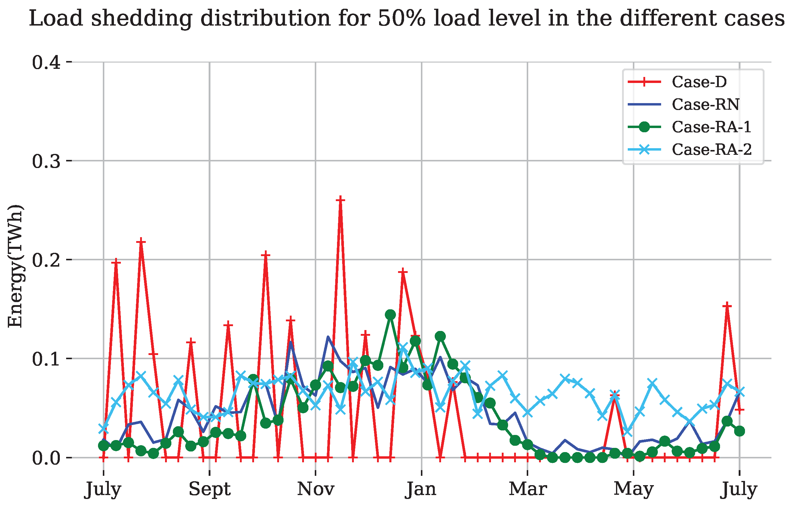
Figure 5 compares the distributions of load shedding in the four cases for a 50% load level increase.

Figure 5.
Load shedding distribution in the four cases for a 50% load level increase.
It is evident from the figure that the stochastic models are more efficient than the deterministic models, which indicates that it would be beneficial to consider uncertainties to avoid the inefficient use of water and incidents of extensive load shedding. The stochastic models distribute the load throughout the year, i.e., small load shedding for an extended period instead of massive load shedding for a short period. The risk-neutral (Case-RN) and the best risk-averse model (Case-RA-1) perform almost equally, with the risk-averse model being slightly better in this particular case. When we examine the risk-averse model (Case-RA-2), considering only the risk with , we have unnecessary load shedding, which leads to the spilling of more water at the end. Therefore, we believe that Case-RA-1 could be the best model for the system. However, it needs further testing and fine-tuning of the parameters. In addition, the model should be tested for a period longer than one year.
4. Conclusions
This paper presents risk-averse and risk-neutral stochastic hydropower planning models in a rolling horizon framework for a one-year planning period developed for the Ethiopian power system. The model is designed to utilize stored water in the rainy season throughout the dry season with minimal load shedding, considering the uncertainties in the inflow. The stochastic model for the first rolling week is compared to its deterministic equivalent model using the quality matrix VSS to show the advantage of solving stochastic problems over deterministic ones. The results show a positive VSS, which is expected for a maximization model.
This paper also considers different risk measures and three cases of risk considerations are compared to account for a reasonable risk measure in the risk-averse problem: Case-a, where the risk considers only the value of stored water; Case-b, where the risk considers only the cost of load shedding; and Case-c, where the risk considers the entire objective function. It is concluded that Case-a with is the best risk measure, and Case-b with is the second-best risk measure considered. Therefore, the two cases are used to develop the risk-averse stochastic model in a weekly rolling horizon framework.
The risk-averse stochastic models are then compared to the risk-neutral stochastic and deterministic models, taking the deterministic model as Case-D, risk-neutral model as Case-RN, and risk-averse model as Case-RA-1 and Case-RA-2. Next, all four cases are simulated in a weekly rolling horizon framework for a one-year planning period using the synthetic historical inflow data of the 2018–2019 planning year as the actual inflow to update the rolling week inflow. Finally, we use 35% and 50% load level increases to compare the performance of the models. The results show that the stochastic models achieve the goal of not having a massive blackout; they distribute load shedding throughout the year. The risk-averse model (Case-RA-1) improves the load shedding situation compared to the other cases for both load level increases, whereas the second risk-averse model (Case-RA-2) results in a lot of load shedding, especially at the 50% load level, which is not sufficiently compensated by the amount of extra stored water at the end of the year.
The results clearly indicate that a stochastic planning model is preferable to a deterministic one. The risk-neutral (Case-RN) and risk-averse (Case-RA-1) models seem to be the most promising planning tools. The case study in this paper only shows a small difference between the risk-neutral and risk-averse models, and it is not possible to draw any definite conclusions about which method is preferable, leaving it open for further interpretation and testing. There are other methods that can be compared with these models, such as the water value method [29] used in the Nordic power system. It could be worth looking at how it works when applied to the Ethiopian power system. Nevertheless, this is outside the scope of this paper.
Therefore, using either of these two stochastic models would be an improvement compared to current planning, which is based on historical generation patterns. The long-term stochastic rolling horizon models can improve the utilization of hydropower, as well as reduce and manage the load-shedding encountered randomly at any time of the year, as well as the draining of reservoirs in the dry season. In addition, they can indicate the need for additional capacity in the system when the load demand exceeds a certain level. Moreover, better planning tools can improve the utilization of hydropower, thereby minimizing generation costs and load shedding.
To further improve long-term planning, it would be interesting to investigate and further test the risk-averse model using a load profile from a different year or simulating a period longer than one year; otherwise, we would not obtain the trade-off between load shedding this year and the energy stored for the following year. Moreover, it would be interesting to apply the water value method to the Ethiopian power system and evaluate its performance in the future.
Author Contributions
Conceptualization, F.G.D. and M.A.; Methodology, F.G.D.; Software, F.G.D.; Validation, F.G.D.; Formal analysis, F.G.D.; Investigation, F.G.D.; Resources, M.A. and G.B.; Data curation, F.G.D.; Writing—original draft, F.G.D.; Writing—review & editing, M.A. and G.B.; Visualization, F.G.D.; Supervision, M.A. and G.B.; Project administration, M.A. and G.B.; Funding acquisition, G.B. All authors have read and agreed to the published version of the manuscript.
Funding
This research was funded by the SIDA-Ethiopia Bilateral program, contribution number 51080124. The APC was funded by the KTH Royal Institute of Technology.
Data Availability Statement
The data presented in this study are available upon request from the corresponding authors.
Conflicts of Interest
The authors declare no conflict of interest.
Nomenclature
| Indices: | |
| i | Index for hydropower plants: |
| m | Index for export area: |
| n | Index for wind power plants: |
| Index for inflow scenarios: | |
| t | Planning period of one year with a weekly time resolution: |
| Parameters: | |
| C | Penalty cost of load shedding |
| Load forecast during week t | |
| Maximal generation in power plant i | |
| I | Number of reservoirs |
| Index set of all power plants downstream of reservoir i | |
| Index set of power plants upstream of reservoir i | |
| Starting contents of reservoir i | |
| Maximal contents of reservoir i | |
| Minimal contents of reservoir i | |
| Minimal contents of reservoir i at the end of planning period T | |
| Power export to area m during week t | |
| M | Number of export areas |
| N | Number of wind power plants |
| Power generation of waste to energy plants during week t | |
| Minimal discharge of power plant i | |
| Maximal discharge of power plant i | |
| T | Number of weeks in the planning horizon |
| Local inflow to reservoir i during week t for scenario | |
| Total wind power generation during week t | |
| Confidence level of Conditional Value at Risk () | |
| risk factor | |
| Production equivalent of power plant i, | |
| Value of future electricity generation | |
| Number of scenarios | |
| Probability of inflow scenario | |
| Variables: | |
| Generation of hydropower plant i during week t for scenario | |
| Contents of reservoir i at the end of week t for scenario | |
| Discharge from power plant i during week t for scenario | |
| Spillage from reservoir i during week t for scenario | |
| Load shedding during week t for scenario | |
| Auxiliary variables for calculating | |
References
- Kaut, M. Scenario generation by selection from historical data. Comput. Manag. Sci. 2021, 18, 411–429. [Google Scholar] [CrossRef]
- Dires, F.G.; Amelin, M.; Bekele, G. Inflow Scenario Generation for the Ethiopian Hydropower System. Water 2023, 15, 500. [Google Scholar] [CrossRef]
- Azad, A.S.; Md, M.S.; Watada, J.; Vasant, P.; Vintaned, J.A.G. Optimization of the hydropower energy generation using Meta-Heuristic approaches: A review. Energy Rep. 2020, 6, 2230–2248. [Google Scholar] [CrossRef]
- Ahlfors, C.; Amelin, M. Weekly planning of hydropower in systems with large volumes and varying power generation: A literature review. In Proceedings of the 2021 IEEE Madrid PowerTech, PowerTech 2021—Conference Proceedings, Madrid, Spain, 28 June–2 July 2021; Institute of Electrical and Electronics Engineers, Inc.: Piscataway, NJ, USA, 2021. [Google Scholar] [CrossRef]
- Hammid, A.T.; Awad, O.I.; Sulaiman, M.H.; Gunasekaran, S.S.; Mostafa, S.A.; Kumar, N.M.; Khalaf, B.A.; Al-Jawhar, Y.A.; Abdulhasan, R.A. A review of optimization algorithms in solving hydro generation scheduling problems. Energies 2020, 13, 2787. [Google Scholar] [CrossRef]
- Gjelsvik, A.; Mo, B.; Haugstad, A. Long- and Medium-term Operations Planning and Stochastic Modelling in Hydro-dominated Power systems Based on Stochastic Dual Dynamic Programming. In Hand Book of Power System I; Springer: Berlin/Heidelberg, Germany, 2010; pp. 33–41. [Google Scholar] [CrossRef]
- Séguin, S.; Fleten, S.E.; Côté, P.; Pichler, A.; Audet, C. Stochastic short-term hydropower planning with inflow scenario trees. Eur. J. Oper. Res. 2017, 259, 1156–1168. [Google Scholar] [CrossRef]
- Vardanyan, Y.; Amelin, M. A sensitivity analysis of short-term hydropower planning using stochastic programming. In Proceedings of the IEEE Power and Energy Society General Meeting, San Diego, CA, USA, 22–26 July 2012; pp. 1–7. [Google Scholar] [CrossRef]
- Fleten, S.E.; Kristoffersen, T.K. Short-term hydropower production planning by stochastic programming. Comput. Oper. Res. 2008, 35, 2656–2671. [Google Scholar] [CrossRef]
- Shang, L.; Li, X.; Shi, H.; Kong, F.; Wang, Y.; Shang, Y. Long-, Medium-, and Short-Term Nested Optimized-Scheduling Model for Cascade Hydropower Plants: Development and Practical Application. Water 2022, 14, 1586. [Google Scholar] [CrossRef]
- Flatabø, N.; Haugstad, A.; Mo, B.; Fosso, O.B. Short-term and Medium-term Generation Scheduling in the Norwegian Hydro System under a Competitive Power Market Structure. In Proceedings of the EPSOM’98 (International Conference on Electrical Power System Operation and Management), Zürich, Switzerland, 23–25 September 1998; pp. 1–18. [Google Scholar]
- Baslis, C.G.; Bakirtzis, A.G. Mid-term stochastic scheduling of a price-maker hydro producer with pumped storage. IEEE Trans. Power Syst. 2011, 26, 1856–1865. [Google Scholar] [CrossRef]
- Côté, P.; Leconte, R. Comparison of Stochastic Optimization Algorithms for Hydropower Reservoir Operation with Ensemble Streamflow Prediction. J. Water Resour. Plan. Manag. 2016, 142, 04015046. [Google Scholar] [CrossRef]
- Quintana, V.H.; Chikhani, A.Y. A Stochastic Model for Mid-Term Operation Planning of Hydro-Thermal Systems with Random Reservoir Inflows. IEEE Trans. Power Appar. Syst. 1981, PAS-100, 1119–1127. [Google Scholar] [CrossRef]
- Scarcelli, R.O.; Zambelli, M.S.; Filho, S.S.; Carneiro, A.A. Aggregated inflows on stochastic dynamic programming for long term hydropower scheduling. In Proceedings of the 2014 North American Power Symposium, NAPS 2014, Pullman, WA, USA, 7–9 September 2014; Institute of Electrical and Electronics Engineers, Inc.: Piscataway, NJ, USA, 2014. [Google Scholar] [CrossRef]
- Rodilla, P.; García-González, J.; Baíllo, Á.; Cerisola, S.; Batlle, C. Hydro resource management, risk aversion and equilibrium in an incomplete electricity market setting. Energy Econ. 2015, 51, 365–382. [Google Scholar] [CrossRef]
- Çavuş, Ö.; Kocaman, A.S.; Yılmaz, Ö. A risk-averse approach for the planning of a hybrid energy system with conventional hydropower. Comput. Oper. Res. 2021, 126, 105092. [Google Scholar] [CrossRef]
- Shapiro, A.; Tekaya, W.; Da Costa, J.P.; Soares, M.P. Risk neutral and risk averse Stochastic Dual Dynamic Programming method. Eur. J. Oper. Res. 2013, 224, 375–391. [Google Scholar] [CrossRef]
- Costley, M.; Feizollahi, M.J.; Ahmed, S.; Grijalva, S. A rolling-horizon unit commitment framework with flexible periodicity. Int. J. Electr. Power Energy Syst. 2017, 90, 280–291. [Google Scholar] [CrossRef]
- Sethi, S.; Sorger, G. A Theory of Rolling Horizon Decision Making. Ann. Oper. Res. 1991, 29, 387–416. [Google Scholar] [CrossRef]
- Devine, M.T.; Bertsch, V. Examining the benefits of load shedding strategies using a rolling-horizon stochastic mixed complementarity equilibrium model. Eur. J. Oper. Res. 2018, 267, 643–658. [Google Scholar] [CrossRef]
- Devine, M.T.; Gabriel, S.A.; Moryadee, S. A rolling horizon approach for stochastic mixed complementarity problems with endogenous learning: Application to natural gas markets. Comput. Oper. Res. 2016, 68, 1–15. [Google Scholar] [CrossRef]
- Bischi, A.; Taccari, L.; Martelli, E.; Amaldi, E.; Manzolini, G.; Silva, P.; Campanari, S.; Macchi, E. A rolling-horizon optimization algorithm for the long term operational scheduling of cogeneration systems. Energy 2019, 184, 73–90. [Google Scholar] [CrossRef]
- Beraldi, P.; Violi, A.; Scordino, N.; Sorrentino, N. Short-term electricity procurement: A rolling horizon stochastic programming approach. Appl. Math. Model. 2011, 35, 3980–3990. [Google Scholar] [CrossRef]
- Dires, F.G.; Amelin, M.; Bekele, G. Deterministic Hydropower Simulation Model for Ethiopia. In Proceedings of the 2021 IEEE Madrid PowerTech, PowerTech 2021—Conference Proceedings, Madrid, Spain, 28 June–2 July 2021. [Google Scholar] [CrossRef]
- Conejo, A.J.; Carrión, M.; Morales, J.M. Risk management. In Decision Making Under Uncertainty in Electricity Markets; Springer: New York, NY, USA, 2010; Chapter 4; pp. 121–152. [Google Scholar] [CrossRef]
- Song, M.; Amelin, M. Price-Maker Bidding in Day-Ahead Electricity Market for a Retailer with Flexible Demands. IEEE Trans. Power Syst. 2018, 33, 1948–1958. [Google Scholar] [CrossRef]
- Birge John, R. The Value of The Stochastic Solution In Stochastic Linear Programs with Fixed Recourse. Math. Program. 1982, 24, 314–325. [Google Scholar] [CrossRef]
- Wangensteen, I. Power System Economics: The Nordic Electricity Market; Tapir Academic Press: Trondheim, Norway, 2006. [Google Scholar]
Disclaimer/Publisher’s Note: The statements, opinions and data contained in all publications are solely those of the individual author(s) and contributor(s) and not of MDPI and/or the editor(s). MDPI and/or the editor(s) disclaim responsibility for any injury to people or property resulting from any ideas, methods, instructions or products referred to in the content. |
© 2023 by the authors. Licensee MDPI, Basel, Switzerland. This article is an open access article distributed under the terms and conditions of the Creative Commons Attribution (CC BY) license (https://creativecommons.org/licenses/by/4.0/).


