Abstract
Current trends in aero-engine design are oriented at designing high-lift low-pressure turbine blades to reduce engine weight and dimensions. Therefore, the validation of numerical methods able to correctly capture the boundary layer transition at cruise conditions with a steady inflow for high-speed blades is of great relevance for turbine designers. The present paper details numerical simulations of a novel open-access high-speed low-pressure turbine test case that are performed using RANS-based transition models. The test case is the SPLEEN C1 cascade, tested in transonic conditions at the von Karman Institute for Fluid Dynamics. Both physics-based and correlation-based transition models are employed to predict blade loading, boundary layer characteristics, and wake development. 2D simulations are run for a wide range of operating conditions ranging from low to high transonic Mach numbers (0.7–0.95) and from low to moderate Reynolds numbers (70,000–120,000). The - transition model shows a good performance over the whole range of simulated operating conditions, thus demonstrating a good capability in both reproducing blade loading and average losses, although the wake’s width is underestimated. This leads to an overestimation of the total pressure deficit in the center of the wake which can exceed experimental measurements by more than 50%. On the other hand, the k-- model achieves satisfactory results at Ma = 0.95, where the boundary layer state is affected by the presence of a weak shock impinging on the blade suction side which thickens the boundary layer, leading to a predicted shape factor equal to five, downstream of the shock. However, at low and moderate Mach numbers, the k-- model predicts long or open separation bubbles contrary to the experimental findings, thus indicating insufficient turbulence production downstream of the boundary layer separation. The slow boundary layer transition in the aft region of the suction side that is exhibited by the k-- model also affects the prediction of the outlet flow, featuring large peaks of a total pressure deficit if compared to both the experimental measurements and the - predictions. For the k-- model, the maximum overestimation of the total pressure deficit is approximately 60%.
1. Introduction
The continuous demand for energy and air transportation leads turbine manufacturers to tackle technological challenges associated with the design of more efficient and sustainable turbomachinery for both propulsion and energy production. In the current trends, the study of high-lift airfoils has sparked major interest thanks to the possibility of reducing the number of blades, maintaining the same work per stage. From an operational point of view, the combination of increased loading with a low chord-based Reynolds number flow, occurring at nominal operating conditions, is likely to cause laminar boundary layer separation which represents one of the major sources of profile losses for the airfoils [1,2]. For this reason, fast and reliable predictive tools are necessary to evaluate design performance in a wide range of operating conditions.
The characterization of high-lift low-pressure turbine cascades in terms of profile and wake losses, both in steady and unsteady conditions, has been extensively analyzed [3,4]. From a numerical standpoint, the prediction of laminar boundary layers can be achieved both by means of high-fidelity methods such as Direct Numerical Simulation (DNS) and Large Eddy Simulation (LES) [5,6,7] and by transition-sensitive Reynolds-Averaged Navier-Stokes (RANS) closures. While LES becomes a more and more widespread tool for the analysis of such configurations in a 3D framework, its adoption from an industrial perspective is still prohibitive because of the large resource requirements. For this reason, RANS models still serve as the most appropriate tool for design optimization [8,9].
RANS-based transition closures can be split into two different classes of models: on one hand, the prediction of the laminar state of the boundary layer is addressed with the concept of intermittency, providing a blending between laminar and turbulent states. To this end, suitable transition onset criteria that allow for complying with different types of transitions (natural, bypass, and separation-induced) are used. In this framework, the most common model was introduced by Menter et al. [10] and later modified by Langtry and Menter [11]. The second class of transition models is physics-based, typically relying on the concept of Laminar Kinetic Energy (LKE) proposed by Mayle and Schulz [12]. This quantity has been used for the development of various transition-sensitive models such as those by Walters and Cokljat [13] and Pacciani et al. [14]. Both approaches have seen extensive use for the simulation of high-lift low-pressure turbine airfoils.
Babajee and Arts [15] applied the - model to the prediction of the T106C low-pressure turbine blade, highlighting the sensitivity of the model to free-stream conditions. The same test case has been used by Minot et al. [16], to assess the effect of numerical implementations of the transition model. The authors studied both the effect of limiters of turbulence production at stagnation points and various correlations for the model’s parameters. More recently, the model has been used for the prediction of 3D flow fields by Pichler et al. [17] and has been adapted for the prediction of a wake-induced transition in steady calculations by Führing et al. [18]. As far as physics-based models are concerned, promising results were obtained both for steady [19] and unsteady computations [20]. The performance of these modeling approaches for the prediction of low-pressure turbine flows has been compared by Pacciani et al. [21] by means of both steady and unsteady computations on high-lift airfoils with a maximum exit isentropic Mach number of 0.65. More recently, Kubacki et al. [22] compared the performance of the - against an algebraic transition model [23] in incompressible flow conditions. Despite the amount of literature devoted to the analysis of RANS-based transition modeling, the performance of such models in a wide range of transonic and low-Reynolds conditions is still an open question. Moreover, the characterization of high-speed, low-pressure turbine blades characterized by the occurrence of weak shocks impinging on the blade suction side (SS) is rarely dealt with within the available literature.
In this paper, predictions by both correlation-based (the -) and physics-based (the k--[24]) transition-sensitive models are compared with experimental data obtained for a transonic low-pressure turbine blade studied in the framework of the EU-funded project SPLEEN [25,26]. While the first model is widely adopted for the prediction of low-Reynolds flows in the turbomachinery community, the k-- has only seen limited applications for this type of flow condition. The accuracy of the models in reproducing the boundary layer behavior is discussed for a wide range of operating conditions obtained by varying both the isentropic outlet Mach number and the isentropic outlet Reynolds number. Conclusions are drawn based on a quantitative comparison between experimental and numerical data. This study identifies the most accurate model to numerically predict transition in high-speed low-pressure turbine blades.
The remainder of the paper is organized as follows. In Section 2, the test case is introduced along with the experimental and numerical methodologies. In Section 2.3, the turbulence models are briefly discussed. In Section 2.4, the mesh sensitivity study performed on the nominal conditions of the rig is presented. The experimental measurements and the numerical predictions are compared in terms of blade loading and losses in Section 3.1 and Section 3.2. Eventually, the predictions of the boundary layer states from both models are discussed to address the main strengths and weaknesses of the two modeling approaches.
2. Test Case
2.1. Experimental Setup
The test case selected for the present activity is the SPLEEN C1 cascade, investigated in the context of the EU-funded project SPLEEN at the von Karman Institute for Fluid Dynamics (BE). The test case has been thoroughly described in ref. [25] and is briefly described here. The SPLEEN C1 cascade is representative of a rotor airfoil of a modern high-speed low-pressure turbine (LPT). The cascade assembly includes 23 blades with a span of 165 mm. The Cascade C1 has been extensively investigated in a wide range of isentropic outlet Mach and Reynolds numbers [26]. During the tests, the freestream turbulence intensity (FSTI) was kept fixed at ∼ using a passive turbulence grid. The mesh size (12 mm) and distance of the latter to the cascade central blade (400 mm) resulted in a measured integral length scale (ILS) of ∼12 mm. The key geometrical characteristics of the airfoil and flow conditions at which the cascade has been investigated are reported in Table 1.

Table 1.
SPLEEN C1 geometry and flow conditions.
The experimental campaign was conducted in the high-speed, low-Reynolds closed loop facility VKI S-1/C. The rig is driven by a 13 stage axial compressor. Near ambient temperature conditions are ensured by means of an air-to-oil heat exchanger. The mass flow rate in the loop is controlled by adjusting the compressor rotational speed and a by-pass valve. The cascade is mounted in the first elbow of the closed loop downstream of the compressor, following a wire mesh and honeycomb that ensure homogeneous inlet flow conditions to the cascade test section.
The cascade mounted in the first elbow of the VKI S-1/C is reported in Figure 1a. The cascade test section, along with the measurement planes in which the measurements have been performed, is reported in Figure 1b. Since the cascade is heavily instrumented [25], only the instrumentation used in the scope of this study is displayed. The turbulence grid location is also highlighted with respect to the instrumentation.
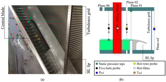
Figure 1.
Experimental setup used to support the current study. (a) SPLEEN Cascade C1 mounted in VKI S-1/C; (b) Test section measurement planes and instrumentation.
Fixed instrumentation is used to live-monitor the flow conditions inside the rig. The isentropic outlet/inlet Mach number and Reynolds number were estimated by means of the inlet total pressure downstream of the grid, outlet/inlet static pressure, and inlet total temperature. The inlet total pressure is not measured; therefore, a correlation to estimate the turbulence grid pressure decay in function of the flow condition was developed to estimate the cascade inlet total pressure based on the measured reference total pressure (upstream of the turbulence grid). Details can be found in [25].
The reference total pressure and temperature were acquired with an absolute pressure sensor (WIKA P-30) and a bare K-type thermocouple. The static pressure is measured at Plane 01 ( upstream of the blade leading edge) and 06 ( downstream of the blade trailing edge). The inlet turbulence measurements were carried out using two hot-wire probes operated in a constant temperature mode. The inlet flow field was characterized at Plane 02 ( upstream of the blade leading edge, LE) by means of a Cobra-shaped 5-hole probe (C5HP). The outlet flow field was surveyed at Plane 06 by means of an L-shaped 5-hole probe (L5HP). The blade loading was computed from pressure tap measurements on the blade surface. The blade suction side (SS) and pressure side (PS) were instrumented with 24 and 17 taps, respectively. Two Scanivalve MPS4264s with ranges of 1 psi and 2.5 psi were used to record the pressure measurements from pneumatic probes and pressure taps at Plane 01, Plane 06, and blade surfaces. Turbulence measurements were recorded by means of an NI card. Surface mounted hot-films were used to survey the BL on the blade PS and SS. Details on the sensor geometry and operating principle are reported by Lopes et al. [27] and by Simonassi et al. [28].
The uncertainty of the quantities computed with the aforementioned instrumentation is presented in Table 2. Both random and systematic uncertainties are expressed with a 95% confidence interval.
Table 2.
Uncertainty of measurements used in this study.
A complete overview of the experimental methods and data generated during the EU project SPLEEN can be retrieved from the open-access experimental database that can be found in ref. [29].
2.2. Numerical Setup
The numerical simulations have been run using HybFlow [30,31,32], a cell-centered finite volume solver developed at the University of Florence (IT), and currently under development at the Politecnico di Torino (IT). The code solves the conservative form of Navier-Stokes equations on hybrid grid topologies. The inviscid fluxes are computed using Roe’s scheme [33], while viscous fluxes are approximated by means of cell gradients plus a penalization term according to [34]. Variable reconstruction is performed by means of a least-square method [35], which achieves second order accuracy on unstructured grid topologies. A steady solution is achieved by means of a pseudo-transient technique based on a damped Newton method with Krylov acceleration. At each numerical time-step, the solution of the linear system is found by means of a preconditioned GMRES solver [36]. The preconditioner is based on a serial 1-level additive Schwarz method, obtained with the ILU(0) factorization of local matrices [37]. For the present investigation, steady simulations were run at a constant CFL of 4.0 and were considered as converged when the density residuals reached a threshold level equal to 10.
Because of the high blade-to-chord ratio, the flow is assumed to be symmetric at mid-span and all simulations are 2D. The inlet of the numerical domain is placed at 1.12 axial chords upstream of the blade LE, namely at Plane 01 of the experimental configuration, while the outlet of the domain is placed one axial chord downstream of the blade TE. The inlet flow field is specified using total pressure, total temperature, and flow angles, while uniform static pressure is imposed at the outlet section. Boundary conditions are chosen in accordance to the experimental non-dimensional rig conditions computed via Equations (1) and (2). Turbulence quantities at the inlet are prescribed in terms of turbulence intensity and integral length scale.
Periodicity is imposed over the lateral boundaries. Hybrid grids were generated using the commercial software Centaur [38]. They consist of triangular elements in the blade passage and quadrilateral elements in the wall vicinity, for a better discretization of the regions characterized by steep gradients. The numerical model of the blade, along with the definitions of blade metal angles () and flow angles (), and the positions of the measurement planes, is shown in Figure 2.
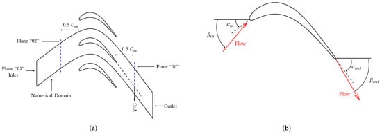
Figure 2.
Blade definition. (a) SPLEEN C1 Blade; (b) Angles Definition.
2.3. Turbulence Modeling
For the present investigation, two different turbulence models have been adopted. The first one is the - transition model [11], in combination with the SST fully turbulent model (Equations (3)–(6)).
The model resorts to the definition of the intermittency variable to simulate the state of the boundary layer. The production of the turbulent kinetic energy is controlled by the parameter , while the transition is controlled by means of the Re at the transition onset. When this variable exceeds a critical threshold (Re), the transition is initiated and the transition length is controlled by the model parameter F. Numerous correlations have been proposed in the literature for the former quantities (e.g., Content and Houdeville [39] and Suluksna et al. [40], among the most relevant ones). In the present paper, the implementation of the model follows the original correlations proposed in [11]. The model is sensitive to the separation-induced transition via the definition of = max(,. The latter model parameter can exceed unity, allowing for a fast transition in the case of separated regions.
The second transition-sensitive turbulence model is the k-- model by Lopez and Walters [24] (Equations (7)–(9)).
The model is a revisited version of the -- transition model by Walters and Cokljat [13], which has been successfully used for the prediction of a high-lift low-pressure turbine airfoil (T106C) by Wang et al. [19]. In this case, the transition is controlled by means of which accounts for fully turbulent, three-dimensional velocity fluctuations. The use of over has the theoretical advantage that the variable can be directly linked to pressure-strain terms, providing a more general framework for physics-based transition modeling. The model activates the transition using the two terms and , which make the model sensitive to bypass and natural transitions. The main difference with the original, LKE-based model is the introduction of a shear stress term similar to the one present in the SST fully turbulent model. Despite the popularity of the --, the k-- has only seen limited applications for the study of turbomachinery flows. To the authors knowledge, the only application for low-pressure turbine blades has been reported by Akolekar et al. [41]. The performance of the k-- model has been compared to the widely-used transition-sensitive RANS closures (LKE-based model [13] and -) and fully turbulent models (k- SST and Spalart-Allmaras [42]). The authors concluded that the k-- yields the most accurate prediction of the boundary layer flow among all the used models. Despite this, the investigation refers to a low-speed low-pressure turbine blade, namely the T106A, working at an outlet isentropic Mach number of ≈0.4.
2.4. Mesh Sensitivity
The sensitivity of the solution to the mesh density was assessed using 4 different grids, ranging from 50 × 10 to 100 × 10 total elements. The analysis was performed for the nominal conditions of the cascade (Ma = 0.9, Re = 70,000) and using the - model. The main characteristics of the meshes are summarized in Table 3. The analysis of the mesh sensitivity is focused on the predictions of both the blade loading (Figure 3a) and the wake development (Figure 3b). Experimental results are also plotted for reference. The effect of the domain discretization on the loading is not evident, neither at LE nor in the formation of the separation bubble on the pressure side. While the simulations manage to capture the acceleration in the front part of the blade up to S/S ≈ 0.6, the diffusion in the rear part of the suction side is slightly faster than the experiments. To conclude, all of the blade loadings obtained by using the investigated meshes converge to the same result.
Table 3.
Mesh characteristics.
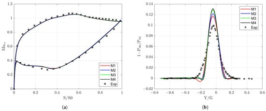
Figure 3.
Mesh sensitivity. (a) Load; (b) Wake. Experimental data retrieved from [29].
Greater differences can be found in the prediction of the wake, both between the meshes and with the experimental measurements. The coarsest mesh predicts the shallowest and thickest wake and the insufficient domain discretization in the wake region is also the probable cause for the slight overshoot in total pressure occurring at Y/G ≈ 0.22. The meshes predict a similar spreading of the wake, with a slightly different peak of the losses. In detail, all the meshes tend to underestimate the spreading, leading to an overestimation of the losses’ peak. This is a typical shortcoming of RANS which has been observed in other numerical works, both for correlation-based and physics-based transition models [43,44]. Despite this, the variability of the results passing from the mesh M2 to the mesh M4 is very low. Eventually, the mesh M3 was considered to be dense enough to properly resolve the flow physics using the selected turbulence models. Full details of the selected mesh can be found in Figure 4.
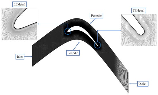
Figure 4.
M3 mesh details.
3. Results and Discussion
In this section, the main findings of the investigation are analyzed. At first, the predictions of the blade loading are compared with experimental measurements, with a particular emphasis on the effect of the Reynolds number and impingement of shocks on the blade suction side. The last sections are dedicated to the discussion of the wake development and the prediction of the boundary layer from both models.
3.1. Blade Loading
The predictions of the blade loading, both for the - and the k-- models, are shown in Figure 5a–c, respectively, for the cases at Re = 70,000, Re = 100,000, and Re = 120,000. Crosses represent experimental points, while numerical predictions from the - and the k-- models are reported with continuous and dashed lines, respectively. The two models present a quite different behavior at low and moderate exit Mach numbers (0.7–0.8), while the predictions are very similar at the highest Mach number (0.95).
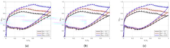
Figure 5.
Blade load: Experimental (cross), - (continuous), and k-- (dashed). (a) Blade load—Re = 70,000; (b) Blade load—Re = 100,000; (c) Blade load—Re = 120,000.
Regarding the -, the prediction of the blade loading follows the experimental trend for the whole range of numerically tested conditions. At the lowest Mach number, the experimental blade loading evidences the occurrence of a separation bubble with a consequent reattachment on the blade suction side. This is clearly seen, especially at the lowest Reynolds number (Figure 5a). For this case, the model fairly predicts the occurrence of the bubble, even though it can be inferred that the size of the separation bubble is too small, which leads to a slight misprediction of the suction side pressure distribution in the range 0.4 < S/S < 0.9. On the other hand, the reattachment region is adequately predicted and the model recovers the experimental diffusion rate in the last part of the suction side closer to the TE. When the Mach number is increased at the same Reynolds number, the model is still able to correctly capture the loading, especially at Ma = 0.95, where both the suction side peak isentropic velocity and the later diffusion are captured properly. At Ma = 0.8 instead, the diffusion is slightly faster than the experimental one. This misprediction was already noticed in Section 2.4. For the medium and the high-Reynolds cases, the performances of the model are approximately the same. At the highest Mach, the load is correctly captured, while at the lowest Mach, the prediction of the rear diffusion after the formation of the separation bubble is correct but the isentropic velocity is slightly underestimated in the central region of the blade. On the contrary, at Ma = 0.8, predictions improve at a higher Re. As far as the k-- is concerned, the model predicts an open separation bubble with no evident reattachment at the lowest Mach numbers. For Ma = 0.95, the results are comparable to the ones obtained with the -, with a fair prediction of the peak velocity point and the later diffusion down to the TE. The k-- also exhibits a worse prediction of the pressure side separation bubble occurring in the region 0.15 < S/S < 0.3 for all tested conditions.
A more detailed analysis of the effect of the Reynolds and Mach numbers on the loading distribution obtained using the - model is presented in Figure 6 and Figure 7, respectively, where the acceleration parameter K and its derivative along the curvilinear coordinate are shown. The figures also report the experimental values of the acceleration parameter only, which have been obtained via a spline interpolation of the experimental insentropic Mach number distribution on the blade suction side.
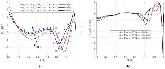
Figure 6.
Acceleration parameter—-. Effect of isentropic outlet Reynolds number. (a) Acceleration parameter; (b) dK/dS.
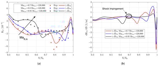
Figure 7.
Acceleration parameter—-. Effect of isentropic outlet Mach number. (a) Acceleration parameter; (b) dK/dS.
As can be observed in Figure 6a, the Reynolds number majorly affects K values in the central region of the blade, but, in general, does not change the loading distribution. The zero of K, which indicates the peak velocity point over the suction side does not change with Reynolds number, while the relative minimum position located in the rear part of the suction side moves downstream along the curvilinear coordinate. This is caused by a change in the separation bubble formation and growth at a different Reynolds number. From a loading perspective, the size and the location of the separation bubble recovery point and reattachment point can be inferred from the distribution of the acceleration parameter [26], even though the exact location of the separation point and the reattachment point are analyzed better by resorting to the wall shear stress. The relative minimum of K approximately indicates the initiation of a separation bubble (at S/S 0.52 for Re = 70,000), while the peak (S/S 0.76 for Re = 70,000) indicates the recovery point, where the separation bubble reaches its maximum size. By increasing the Reynolds number, the peak moves upstream, and the acceleration curve is flatter, indicating a lower size of the bubble. Moreover, the diffusion in the rear part at a lower Reynolds is faster, due to a later reattachment of the bubble itself. This point can be approximately located at the peak of the acceleration derivative (Figure 6b), which moves from S/S = 0.85 at Re = 120,000 to S/S = 0.95 at Re = 70,000.
The Mach number mainly affects the acceleration in the front part, bringing the peak velocity point from S/S 0.37 for Ma = 0.7 to S/S 0.61 for Ma = 0.95, as can be seen in Figure 7a by tracking the K = 0 abscissa for the three Mach numbers. Also, with an increase of the Mach number, the acceleration derivative tends to be 0, downstream of the velocity peak at S/S 0.7 (see Figure 7b), and the K curve tends to be flatter in the high-Mach case if compared to the low-Mach number case. This is caused by the fact that the separation bubble tends to be suppressed and does not retain a major effect on the acceleration over the profile. Another major feature of the high-Mach case is the presence of a small bump in close to S/S 0.7. This is not present in the other cases and is due to the presence of a shock in the throat section of the cascade, as shown in Figure 8 using the numerical Schlieren.
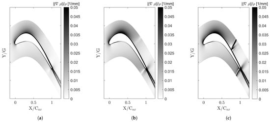
Figure 8.
Numerical Schlieren. (a) Ma = 0.7, Re = 120,000; (b) Ma = 0.9, Re = 120,000; (c) Ma = 0.95, Re = 120,000.
The simulations underestimate the experimental acceleration parameter at a low-Mach (Figure 6) for all Reynolds numbers in the front region up to S/S = 0.7. At Re = 70,000, numerical predictions underestimate the acceleration parameter until S/S = 0.91, thus including the minimum value. At the highest outlet Reynolds number, the underestimation stops at S/S = 0.7 and the minimum value is overestimated. The best prediction in the aft region is obtained at the medium outlet Reynolds number, where the minimum value of the acceleration parameter is retrieved correctly.
A better agreement between simulations and experiments in the front part of the blade is found at Re = 120,000 (Figure 7). For the medium Mach case, the simulations correctly capture the experimental values up to S/S = 0.8. Experiments show an almost constant diffusion rate in the region 0.85 < S/S < 0.95, while the simulations show a clear minimum at S/S = 0.91 with a less smoother trend. At the highest Mach number, simulations overestimate the acceleration in the region 0.51 < S/S < 0.61. Moreover, the diffusion rate is faster in the region 0.68 < S/S < 0.88, where the acceleration parameter is underestimated. Finally, an overestimation is found in high-Mach conditions for S/S > 0.88.
3.2. Wake Prediction
The flow field measured at Plane 06 was compared to the numerical results from both models in terms of the mass-flow-averaged total pressure loss and deviation angle (Equation (10)) in Table 4 and Table 5.
Table 4.
Total pressure losses—Plane 06.
Table 5.
Deviation—Plane 06.
Regarding the total pressure losses, both models manage to satisfactorily predict the experimental values. The maximum discrepancy occurs for the Ma = 0.95 Re = 70,000 case when using the - model. The two models tend to overestimate the losses, but in both cases, they manage to correctly retrieve the experimental trend which sees an increase of the losses with Ma. Moreover, both models predict a reduction of losses when Re is increased from 70,000 to 120,000 for Ma = 0.9. The same trend has been found for the deviation angle. Table 5 also reports the experimental uncertainty over the measured angle. It can be observed that the predictions obtained with the - model are generally in better agreement than the ones produced by the k-- in terms of the deviation angle.
Figure 9 shows the predicted shape of the wake, compared with the experimental measurements. The effect of the Reynolds number is shown in Figure 9a, where the wakes are compared at Ma = 0.9. Both models overpredict the peak of losses at the center of the wake and underestimate the wake spreading, as already mentioned in Section 2.4. The - model performs better than the k-- model, especially at Re = 120,000, with a maximum deviation from the experimental measurement equal to ≈0.045. However, the - exhibits very little sensitivity to the Reynolds number at Ma = 0.9. Indeed, the peak of the losses only reduces by ≈0.01 when the outlet Reynolds number is increased from 70,000 to 120,000. The experiments show a reduction of ≈0.02. A similar reduction in the peak of losses is found in the predictions from the k-- model (≈0.023).
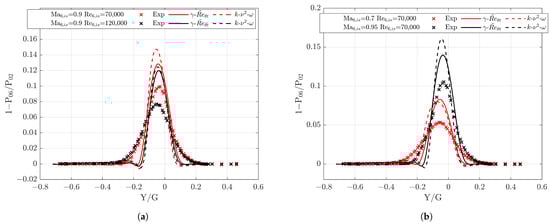
Figure 9.
Wake prediction. (a) Effect of the Reynolds number; (b) Effect of Mach number.
The effect of the Mach number is instead shown in Figure 9b, for Re = 70,000. The two models perform similarly for the lowest isentropic Mach (0.7), but the k-- performs sensibly worse at the highest Mach number, predicting a very thin wake, with a very high peak in the losses which exceeds the experimental one by more than 50%. The - also retrieves the experimental increase in the peak of losses (≈0.05) passing from Ma = 0.7 to Ma = 0.95. It is worth mentioning that the k-- wakes are slightly misaligned with respect to the experimental one, being a little closer to the blade SS. On the other hand, the - correctly predicts the position of the wake for all the combinations of outlet isentropic Mach and Reynolds numbers. It must be underlined that the two models have a similar treatment of the wake region, both implementing a shear stress transport term, so the different prediction of the wake region is to be addressed to the different state of the boundary layer in the rear part of the SS, which affects the wake growth and position, especially in the case of open and long separation bubbles. This topic will be discussed in Section 3.3, where the boundary layers predicted by the two models will be compared.
3.3. Boundary Layer Analysis
In this section, the prediction of the boundary layer parameters from both models are analyzed and compared to the main experimental findings.
3.3.1. Separation and Reattachment Prediction
In order to understand the performance of the two models in the prediction of the separation point and the reattachment location, the Reynolds number at the separation point Re and the Reynolds number at the reattachment point Re are compared with the experimental correlations from Hatman and Wang [45]. The comparison is carried out for low and moderate Mach numbers and, as far as the reattachment point is concerned, only for the - model, which consistently predicts the reattachment of the separation bubble. The k-- predicts a reattachment point only for the highest Reynolds, so this part of the analysis has been skipped.
The definition of the separation and reattachment location is carried out resorting to the points where the wall shear stress changes sign. While the shape of the acceleration parameter gives an insight on the separation, recovery, and reattachment points based on the loading of the blade as discussed in Section 3.1, the prediction of both the separation point and the reattachment point is not properly accurate as shown in Figure 10a. The separation and reattachment locations predicted from the acceleration parameter are compared to the locations obtained from an analysis of the shear stress for the low-Mach, low-Reynolds case, and the - model. The separation and reattachment points obtained from the acceleration parameter are indicated as S and R, respectively, while the separation and reattachment points from the wall shear stress are indicated as S and R. The reattachment point R is located in correspondence of the peak of the acceleration parameter derivative (the blue curve). The use of the acceleration parameter leads to a slight over-prediction of the separation bubble length. This is due to both an anticipated position of the separation point and a slight overestimation in the position of the reattachment when compared to the data obtained from the wall shear stress.
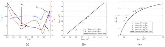
Figure 10.
Bubble prediction. (a) Prediction of the separation and reattachment point: Ma = 0.7, Re = 70,000; (b) Comparison with experimental correlation [45]: reattachment point; (c) Comparison with experimental correlation [45]: separation point.
The bubble size is compared with experimental correlations in Figure 10b. The experimental correlations are those of Hatman and Wang [45], obtained for a flat plate operating in subsonic conditions. While the numerical trend is in good agreement with the experimental one, the size of the separation bubble length is underpredicted, especially in the case of low-Reynolds number (bottom-left region of the plot). It must be said that the correlations were obtained for a very low free-stream turbulence intensity (TI < 0.6%), which can explain the difference with respect to this particular test case.
In Figure 10c, the separation Reynolds number is compared to the acceleration parameter at the separation location. In this case, both the models predict an earlier separation with respect to experimental correlations, even though the origin of this disagreement could not be identified.
3.3.2. Wall Shear Stress
In Figure 11, the normalized wall shear stress obtained from the numerical simulations is compared to the quasi-shear stress measured during the experimental campaign [29] for a set of three different combinations of Ma and Re. The wall shear stress is normalized with respect to the value observed at S/S = 0.038, which corresponds to the first available measurement point on the suction side. The comparison between the numerical shear stress and the experimental quasi-shear stress values is primarily qualitative. It addresses the ability of both models in capturing shear stress variations associated to flow acceleration/deceleration, the occurrence of the separation bubble, and the impinging shock on the blade suction side. Separation and reattachment locations can be identified as the points where the absolute value of the shear stress is null. The isentropic Mach number distributions are also added for convenience.
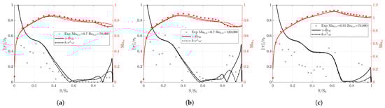
Figure 11.
Normalized wall shear stress. (a) Ma = 0.7 Re = 70,000; (b) Ma = 0.7 Re = 120,000; (c) Ma = 0.95 Re = 70,000.
Concerning the - model, for the low-Mach, low-Reynolds case (Figure 11a), the numerical predictions agree with the experimental trend over the whole length of the suction side up to S/S 0.8. At this point, the model predicts the start of the transition induced by the growth of the separation bubble, which can be seen from the increase of the magnitude of the wall shear stress, with a later reattachment occurring at S/S 0.89. After the reattachment, the model tends to overestimate the growth of , overpredicting the values close to the TE.
At the low-Mach, high-Reynolds (Figure 11b), the prediction is satisfactory up to the separation point that occurs at S/S 0.59. In comparison with the experimental data, the prediction of the wall shear stress in the separation bubble region (0.59 < S/S < 0.84) is very good, but the transition occurs slower and a turbulent state of the boundary layer is almost reached further downstream, close to the TE (see also the discussion about the shape factor in Figure 12a, Section 3.3.2).
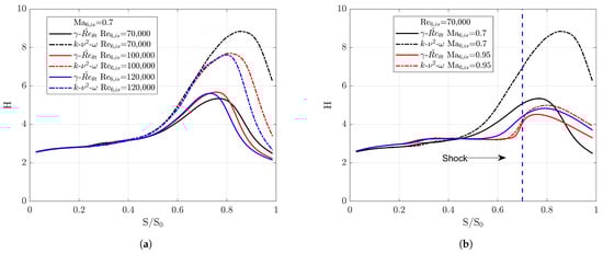
Figure 12.
Comparison of Shape Factor. (a) Effect of Reynolds number; (b) Effect of Mach number.
At the high-Mach, low-Reynolds instead (Figure 11c), experimental data are more scattered. However, both the trend in the accelerating region S/S < 0.6 and the sudden drop in the wall shear stress after the velocity peak at S/S 0.6 are correctly captured by both models. In the region 0.7 < S/S < 0.84, both the experiments and the CFD predict a very low value of the wall shear stress. This is due to the impinging of the shock on the suction side, shown by means of the numerical Schlieren in Figure 8 and by means of the acceleration parameter in Figure 6. When the shock impinges on the suction side, the increase in pressure favors the thickening of the boundary layer with a consequent low value of the wall shear stress. This aspect is investigated further in Figure 12 in Section 3.3.2. At a high-Mach low-Reynolds, the k-- model retains a similar behavior compared to the -. The major difference is the prediction of a very thin separation bubble in the region 0.71 < S/S < 0.87, which is not evidenced by the - model. It is worth mentioning that the size of the separation bubble is so small that it does not retain any effect on the loading.
On the other hand, the two models behave quite differently at the low-Mach, as can be observed in Figure 11a,b. For Re = 70,000, the k-- model predicts an open separation bubble with no reattachment. While the comparison with the experimental shear stress is reasonably good (in terms of absolute values), the misprediction of the loading in the rear part of the suction side shows that the bubble is actually closed. The same behavior can be seen at a high-Reynolds (Re = 120,000). In this case, the k-- predicts a reattachment point after separation (S/S 0.94), occurring significantly later than the reattachment point predicted by the - (S/S 0.84). Despite a better prediction of the absolute values of the wall shear stress in the separation bubble region, the loading shows an overestimation of the reattachment location from the k-- model. It must be noted that the main difference between the two models in terms of wall shear stress occurs in the prediction of the reattachment location (if present), while the results in the laminar region up to the velocity peak are similar.
3.3.3. Shape Factor
The effect of the Reynolds number and Mach number on the prediction of the boundary layer shape factor (H = ) is shown in Figure 12a,b, respectively. The models predict a different state of the boundary layer for all cases.
At Ma = 0.7, the models have the same behavior in the accelerating region of the suction side up to S/S 0.4, close to the velocity peak. The boundary layer tends to become thicker downstream of the velocity peak, due to the adverse pressure gradient, and eventually separates. Concerning the k-- model, the separation bubble is much bigger, leading to almost twice the shape factor compared to the one predicted using the -. In fact, looking at the shear stress values reported in Figure 11a, for the k-- model, the separation bubble tends to reattach at the intermediate and highest Reynolds, while the same does not occur at the lowest Reynolds which shows a shape factor of six in the TE region. On the contrary, the - model always predicts a reattachment, with a near turbulent shape factor (≈2) at the TE [46] for all the Reynolds numbers.
The different behavior of the two models in presence of a separation bubble is analyzed in Figure 13, where the intermittency contour and the ratio are shown. It is worth explaining that the ratio is equal to 1 in fully turbulent regions (where ) while the transition is not fully complete when the ratio is <1. The analysis is performed for the low-Mach, low-Reynolds case.
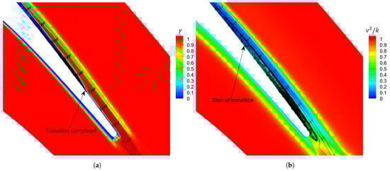
Figure 13.
Separation-induced transition—Ma = 0.7 Re = 70,000. (a) -; (b) k--.
After the occurrence of the separation bubble, the - model predicts a fully turbulent boundary layer at S/S 0.9. This occurs slightly before the reattachment of the separation bubble. This fast reaction of the model to the separation bubble is due to the term that controls the production of turbulent kinetic energy. On the contrary, for the k-- model, the boundary layer transition starts at S/S 0.8, well after the initiation of the separation bubble at S/S 0.55. Eventually, it is not completed before reaching the TE of the blade. The reason for this behavior is that the k-- model is not sensitized to a separation-induced mechanism, but only to the bypass transition (occurring at high free-stream turbulence intensity) via the term and to the natural transition (which is an inherently slow process) via the term .
Concerning the effect of the Mach number, the boundary layer shape factors at Re = 70,000 are shown in Figure 12b for low and high-Mach conditions. At Ma = 0.95, the shape factor reaches a peak at S/S = 0.33, slightly before the velocity peak (S/S 0.45). After that, when the shock impinges on the suction side at S/S 0.7, the boundary layer shape factor grows above four, and then decreases until the TE. The trend is the same for both models. For the -, the boundary layer predicted at a low-Mach has a lower shape factor with respect to the one at a high-Mach for S/S > 0.87. This is caused by the fact that the occurrence of the separation bubble at Ma = 0.7 favors both the transition of the boundary layer to a turbulent state and inherently, a lower shape factor at the TE region. As shown in Figure 14, no evident transition occurs at Ma = 0.95, so the boundary layer remains in a laminar state after the impingement of the weak shock on the blade suction side.
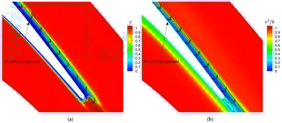
Figure 14.
Suction side boundary layer—Ma = 0.95 Re = 70,000. (a) -; (b) k--.
4. Conclusions
In this paper, the performance of two different transition-sensitive RANS closure models was compared for a low-pressure turbine blade tested in the framework of the EU-funded SPLEEN project for a wide range of operating conditions. The selected models are the commonly adopted - and the k--. The numerical predictions are compared with the experimentally measured load and wake distributions, while a deep analysis of the boundary layer state is performed to address the main differences between the two closure models.
The - performs well in all operating regimes, with a satisfactory prediction of both the blade loading and the averaged losses and deviations at the outlet measurement plane. Despite this, the wake is not mixed enough with the main flow, leading to a narrow distribution with an overprediction of the total pressure loss over its centerline. The prediction of the separation and reattachment position is compared to experimental correlations, showing a good agreement in terms of the trend. Despite this, the separation point occurs too early.
Contrarily to available literature findings at low-Mach conditions (namely Ma = 0.4 [41]), the k-- model performs sensibly worse than the - in transonic regimes with an isentropic outlet Mach number ranging from 0.7 to 0.8. The model predicts long/open separation bubbles, failing to correctly retrieve the experimental blade loading, especially at Re = 70,000–100,000. The model also predicts a slight misalignment of the wake, with large peaks of losses over the centerline. As a matter of fact, the wake is closer to the blade suction side compared to both the experimental findings and the - predictions. It is shown that the main difference between the two models is related to the slow reaction of the k--, to the occurrence of a separation bubble, causing a thick boundary layer in the aft part of the suction side. The boundary layer state eventually affects both the loading and the wake’s prediction.
At Ma = 0.95, the cascade is characterized by the presence of a weak shock impinging over the blade suction side. Its effect is analyzed both in terms of an acceleration parameter and boundary layer state at Re = 70,000. The weak shock causes a thick, laminar boundary layer, with the occurrence of a very small separation bubble for the k-- model. In these conditions, the two models yield similar predictions, both in terms of the loading and boundary layer state upstream of the shock. However, the - predicts a thinner boundary layer in the diffusive region of the blade suction side, which leads to a better prediction of the downstream wake.
It is concluded that the - offers the most accurate predictions in the range of simulated outlet isentropic Mach and Reynolds numbers. On the other hand, it is suggested that the performance of the k-- model for the prediction of high-speed low pressure turbine airfoils could be improved by sensitizing the model to a separation-induced transition.
Author Contributions
Conceptualization, N.R. and G.L., S.S., D.A.M. and S.L.; methodology, N.R., G.L., S.S., S.L. and D.A.M.; software, N.R. and S.S.; validation, N.R., G.L. and S.L.; formal analysis, N.R. and G.L.; investigation, N.R. and G.L.; resources, S.S., D.A.M. and S.L.; data curation, G.L. and S.L.; writing—original draft preparation, N.R. and G.L.; writing—review and editing, N.R., G.L., S.S., S.L. and D.A.M.; visualization, N.R. and G.L.; supervision, S.S., D.A.M. and S.L.; project administration, S.S., D.A.M. and S.L.; funding acquisition, S.L. All authors have read and agreed to the published version of the manuscript.
Funding
The experimental campaign of the SPLEEN project was funded by the Clean Sky 2 Joint Undertaking under the European Union’s Horizon 2020 research and innovation program under the grant agreement 820883.
Data Availability Statement
The experimental data presented in this study are openly available in Zenodo at https://doi.org/10.5281/zenodo.8075795, accessed on 1 July 2023.
Acknowledgments
The authors are grateful to Francesco Martelli for the support provided in the development of the HybFlow solver during his work period at the University of Florence (IT). We acknowledge the CINECA award under the ISCRA initiative, for the availability of high performance computing resources and support. The authors are also grateful to the von Karman Institute for Fluid Dynamics for hosting Nicola.
Conflicts of Interest
The authors declare no conflict of interest.
Abbreviations
The following abbreviations are used in this manuscript:
| Abbreviations | |
| C | Blade true chord |
| Blade axial chord | |
| C5HP | Cobra-shaped five-hole probe |
| d | Deviation angle |
| DNS | Direct numerical simulation |
| FSTI | Freestream turbulence intensity |
| G | Pitch |
| GMRES | Generalized Minimal Residual |
| H | Shape factor |
| HF | Surface mounted hot-film sensor |
| i | Incidence angle |
| ILS | Integral length scale |
| k | Heat capacity ratio |
| K | Acceleration parameter |
| LE | Leading edge |
| LES | Large-Eddy simulation |
| LKE | Laminar kinetic energy |
| L5HP | L-shaped five-hole probe |
| Ma | Mach number |
| PS | Pressure side |
| P | Total pressure |
| RANS | Reynolds-Averaged Navier-Stokes |
| Re | Reynolds number |
| Re | Reynolds number at separation point |
| Re | Reynolds number at reattachment point |
| S | Curvilinear coordinate |
| S | Curve length |
| SS | Suction side |
| SST | Shear stress transport |
| TE | Trailing edge |
| TI | Turbulence intensity |
| U | Experimental uncertainty |
| V | Velocity magnitude |
| Y | Pitchwise coordinate |
| Subscripts and Superscripts | |
| Freestream | |
| Relative to the inlet | |
| Isentropic | |
| Metallic | |
| Relative to the outlet | |
| Random | |
| Systematic | |
| 2 | Relative to Plane 02 |
| 6 | Relative to Plane 06 |
| Greek Letters | |
| Blade metal angle | |
| Flow angle | |
| Displacement thickness | |
| Kinematic viscosity | |
| Density | |
| Wall shear stress | |
| Reference wall shear stress | |
| Momentum thickness | |
References
- Curtis, E.M.; Hodson, H.P.; Banieghbal, M.R.; Denton, J.D.; Howell, R.J.; Harvey, N.W. Development of Blade Profiles for Low-Pressure Turbine Applications. J. Turbomach. 1997, 119, 531–538. [Google Scholar] [CrossRef]
- Lou, W.; Hourmouziadis, J. Separation Bubbles Under Steady and Periodic-Unsteady Main Flow Conditions. J. Turbomach. 2000, 122, 634–643. [Google Scholar] [CrossRef]
- Michálek, J.; Monaldi, M.; Arts, T. Aerodynamic Performance of a Very High Lift Low Pressure Turbine Airfoil (T106C) at Low Reynolds and High Mach Number with Effect of Free Stream Turbulence Intensity. J. Turbomach. 2012, 134, 061009. [Google Scholar] [CrossRef]
- Brunner, S.; Fottner, L.; Schiffer, H.P. Comparison of Two Highly Loaded Low Pressure Turbine Cascades Under the Influence of Wake-Induced Transition. In Proceedings of the ASME Turbo Expo 2000: Power for Land, Sea, and Air, Munich, Germany, 8–11 May 2000; Volume 3: Heat Transfer, Electric Power; Industrial and Cogeneration. p. V003T01A073. [Google Scholar] [CrossRef]
- Michelassi, V.; Wissink, J.; Rodi, W. Analysis of DNS and LES of Flow in a Low Pressure Turbine Cascade with Incoming Wakes and Comparison with Experiments. Flow Turbul. Combust. 2002, 69, 295–329. [Google Scholar] [CrossRef]
- de Wiart, C.C.; Hillewaert, K.; Geuzaine, P. DNS of a Low Pressure Turbine Blade Computed with the Discontinuous Galerkin Method. In Proceedings of the ASME Turbo Expo 2012: Turbine Technical Conference and Exposition, Copenaghen, Denmark, 11–15 June 2012; Volume 8: Turbomachinery, Parts A, B, and C, pp. 2101–2111. [Google Scholar] [CrossRef]
- Garai, A.; Diosady, L.; Murman, S.; Madavan, N. DNS of Flow in a Low-Pressure Turbine Cascade Using a Discontinuous-Galerkin Spectral-Element Method. In Proceedings of the ASME Turbo Expo 2015: Turbine Technical Conference and Exposition, Montreal, QC, Canada, 15–19 June 2015; Volume 2B: Turbomachinery, p. V02BT39A023. [Google Scholar] [CrossRef]
- Baert, L.; Chérière, E.; Sainvitu, C.; Lepot, I.; Nouvellon, A.; Leonardon, V. Aerodynamic Optimization of the Low-Pressure Turbine Module: Exploiting Surrogate Models in a High-Dimensional Design Space. J. Turbomach. 2020, 142, 031005. [Google Scholar] [CrossRef]
- Giovannini, M.; Rubechini, F.; Marconcini, M.; Arnone, A.; Bertini, F. Reducing Secondary Flow Losses in Low-Pressure Turbines: The “Snaked” Blade. Int. Turbomach. Propuls. Power 2019, 4, 28. [Google Scholar] [CrossRef]
- Menter, F.R.; Langtry, R.B.; Likki, S.R.; Suzen, Y.B.; Huang, P.G.; Völker, S. A Correlation-Based Transition Model Using Local Variables—Part I: Model Formulation. J. Turbomach. 2004, 128, 413–422. [Google Scholar] [CrossRef]
- Langtry, R.B.; Menter, F.R. Correlation-Based Transition Modeling for Unstructured Parallelized Computational Fluid Dynamics Codes. AIAA J. 2009, 47, 2894–2906. [Google Scholar] [CrossRef]
- Mayle, R.E.; Schulz, A. The Path to Predicting Bypass Transition. In Proceedings of the ASME 1996 International Gas Turbine and Aeroengine Congress and Exhibition, Birmingham, UK, 10–13 June 1996; Volume 1: Turbomachinery, p. V001T01A065. [Google Scholar] [CrossRef]
- Walters, D.K.; Cokljat, D. A Three-Equation Eddy-Viscosity Model for Reynolds-Averaged Navier–Stokes Simulations of Transitional Flow. J. Fluids Eng. 2008, 130, 121401. [Google Scholar] [CrossRef]
- Pacciani, R.; Marconcini, M.; Fadai-Ghotbi, A.; Lardeau, S.; Leschziner, M.A. Calculation of High-Lift Cascades in Low Pressure Turbine Conditions Using a Three-Equation Model. J. Turbomach. 2010, 133, 031016. [Google Scholar] [CrossRef]
- Babajee, J.; Arts, T. Investigation of the Laminar Separation-Induced Transition with the - Transition Model on Low-Pressure Turbine Rotor Blades at Steady Conditions. In Proceedings of the ASME Turbo Expo 2012: Turbine Technical Conference and Exposition, Copenhagen, Denmark, 11–15 June 2012; Volume 8: Turbomachinery, Parts A, B, and C, pp. 1167–1178. [Google Scholar] [CrossRef]
- Minot, A.; de Saint Victor, X.; Marty, J.; Perraud, J. Advanced Numerical Setup for Separation-Induced Transition on High-Lift Low-Pressure Turbine Flows Using the - Model. In Proceedings of the ASME Turbo Expo 2015: Turbine Technical Conference and Exposition, Montreal, QC, Cnanda, 15–19 June 2015; Volume 2B: Turbomachinery, p. V02BT39A010. [Google Scholar] [CrossRef]
- Pichler, R.; Zhao, Y.; Sandberg, R.; Michelassi, V.; Pacciani, R.; Marconcini, M.; Arnone, A. Large-Eddy Simulation and RANS Analysis of the End-Wall Flow in a Linear Low-Pressure Turbine Cascade, Part I: Flow and Secondary Vorticity Fields Under Varying Inlet Condition. J. Turbomach. 2019, 141, 121005. [Google Scholar] [CrossRef]
- Führing, A.; Kožulović, D.; Bode, C.; Franke, M. Steady State Modeling of Unsteady Wake Induced Transition Effects in a Multistage Low Pressure Turbine. In Proceedings of the ASME Turbo Expo 2020: Turbomachinery Technical Conference and Exposition, Virtual, Online, 21–25 September 2020; Volume 2C: Turbomachinery, p. V02CT35A012. [Google Scholar] [CrossRef]
- Wang, X.; Cui, B.; Xiao, Z. Numerical investigation on ultra-high-lift low-pressure turbine cascade aerodynamics at low Reynolds numbers using transition-based turbulence models. J. Turbul. 2021, 22, 114–139. [Google Scholar] [CrossRef]
- Pacciani, R.; Marconcini, M.; Arnone, A.; Bertini, F. URANS Prediction of the Effects of Upstream Wakes on High-lift LP Turbine Cascades Using Transition-sensitive Turbulence Closures. Energy Procedia 2014, 45, 1097–1106. [Google Scholar] [CrossRef]
- Pacciani, R.; Marconcini, M.; Arnone, A.; Bertini, F. Predicting High-Lift Low-Pressure Turbine Cascades Flow Using Transition-Sensitive Turbulence Closures. J. Turbomach. 2013, 136, 051007. [Google Scholar] [CrossRef]
- Kubacki, S.; Jonak, P.; Dick, E. Evaluation of an algebraic model for laminar-to-turbulent transition on secondary flow loss in a low-pressure turbine cascade with an endwall. Int. J. Heat Fluid Flow 2019, 77, 98–112. [Google Scholar] [CrossRef]
- Kubacki, S.; Dick, E. An algebraic intermittency model for bypass, separation-induced and wake-induced transition. Int. J. Heat Fluid Flow 2016, 62, 344–361. [Google Scholar] [CrossRef]
- Lopez, M.; Walters, D.K. Prediction of transitional and fully turbulent flow using an alternative to the laminar kinetic energy approach. J. Turbul. 2016, 17, 253–273. [Google Scholar] [CrossRef]
- Simonassi, L.; Lopes, G.; Gendebien, S.; Torre, A.F.M.; Patinios, M.; Lavagnoli, S.; Zeller, N.; Pintat, L. An Experimental Test Case for Transonic Low-Pressure Turbines—Part I: Rig Design, Instrumentation and Experimental Methodology. In Proceedings of the ASME Turbo Expo 2022: Turbomachinery Technical Conference and Exposition, Rotterdam, The Netherlands, 13–17 June 2022; Volume 10B: Turbomachinery—Axial Flow Turbine Aerodynamics, Deposition, Erosion, Fouling, and Icing; Radial Turbomachinery Aerodynamics. p. V10BT30A012. [Google Scholar] [CrossRef]
- Lopes, G.; Simonassi, L.; Torre, A.F.M.; Patinios, M.; Lavagnoli, S. An Experimental Test Case for Transonic Low-Pressure Turbines—Part 2: Cascade Aerodynamics at On- and Off-Design Reynolds and Mach Numbers. In Proceedings of the ASME Turbo Expo 2022: Turbomachinery Technical Conference and Exposition, Rotterdam, The Netherlands, 13–17 June 2022; Volume 10B: Turbomachinery—Axial Flow Turbine Aerodynamics, Deposition, Erosion, Fouling, and Icing; Radial Turbomachinery Aerodynamics. p. V10BT30A027. [Google Scholar] [CrossRef]
- Lopes, G.; Simonassi, L.; Lavagnoli, S. Impact of Unsteady Wakes on the Secondary Flows of a High-Speed Low-Pressure Turbine Cascade. Int. J. Turbomach. Propuls. Power 2023, 8, 36. [Google Scholar] [CrossRef]
- Simonassi, L.; Lopes, G.; Lavagnoli, S. Effects of Periodic Incoming Wakes on the Aerodynamics of a High-Speed Low-Pressure Turbine Cascade. Int. J. Turbomach. Propuls. Power 2023, 8, 35. [Google Scholar] [CrossRef]
- Lavagnoli, S.; Lopes, G.; Simonassi, L.; Torre, A.F.M. SPLEEN—High Speed Turbine Cascade—Test Case Database. 2023. Available online: https://zenodo.org/records/8075795 (accessed on 1 July 2023).
- Adami, P.; Salvadori, S.; Chana, K.S. Unsteady Heat Transfer Topics in Gas Turbine Stages Simulations. In Proceedings of the ASME Turbo Expo 2006: Power for Land, Sea, and Air, Barcelona, Spain, 8–11 May 2006; Volume 6: Turbomachinery, Parts A and B, pp. 1733–1744. [Google Scholar] [CrossRef]
- Adami, P.; Belardini, E.; Martelli, F.; Michelassi, V. Unsteady Rotor/Stator Interaction: An Improved Unstructured Approach. In Proceedings of the ASME Turbo Expo 2001: Power for Land, Sea, and Air, New Orleans, LA, USA, 4–7 June 2001; Volume 1: Aircraft Engine, Marine; Turbomachinery; Microturbines and Small Turbomachinery. p. V001T03A051. [Google Scholar] [CrossRef]
- Adami, P.; Martelli, F.; Michelassi, V. Three-Dimensional Investigations for Axial Turbines by an Implicit Unstructured Multi-Block Flow Solver. In Proceedings of the ASME Turbo Expo 2000: Power for Land, Sea, and Air, Munich, Germany, 8–11 May 2000; Volume 1: Aircraft Engine, Marine; Turbomachinery; Microturbines and Small Turbomachinery. p. V001T03A108. [Google Scholar] [CrossRef]
- Roe, P. Approximate Riemann solvers, parameter vectors, and difference schemes. J. Comput. Phys. 1981, 43, 357–372. [Google Scholar] [CrossRef]
- Ollivier-Gooch, C.; Jalali, A. Accuracy Assessment of Finite Volume Discretizations of Diffusive Fluxes on Unstructured Meshes. In Proceedings of the 50th AIAA Aerospace Sciences Meeting Including the New Horizons Forum and Aerospace Exposition, Nashville, Tennessee, 9–12 January 2012. [Google Scholar] [CrossRef]
- Ollivier-Gooch, C.; Ollivier-Gooch, C. High-order ENO schemes for unstructured meshes based on least-squares reconstruction. In Proceedings of the 35th Aerospace Sciences Meeting and Exhibit, Reno, NV, USA, 6–9 January 1997. [Google Scholar] [CrossRef]
- Saad, Y.; Schultz, M.H. GMRES: A Generalized Minimal Residual Algorithm for Solving Nonsymmetric Linear Systems. SIAM J. Sci. Stat. Comput. 1986, 7, 856–869. [Google Scholar] [CrossRef]
- Xu, S.; Mohanamuraly, P.; Wang, D.; Müller, J.D. Newton–Krylov Solver for Robust Turbomachinery Aerodynamic Analysis. AIAA J. 2020, 58, 1320–1336. [Google Scholar] [CrossRef]
- Available online: https://www.centaursoft.com/ (accessed on 1 February 2023).
- Content, C.; Houdeville, R. Application of the - laminar-turbulent transition model in Navier-Stokes computations. In Proceedings of the 40th Fluid Dynamics Conference and Exhibit, Chicago, IL, USA, 28 June–1 July 2010. [Google Scholar] [CrossRef]
- Suluksna, K.; Dechaumphai, P.; Juntasaro, E. Correlations for modeling transitional boundary layers under influences of freestream turbulence and pressure gradient. Int. J. Heat Fluid Flow 2009, 30, 66–75. [Google Scholar] [CrossRef]
- Akolekar, H.D.; Weatheritt, J.; Hutchins, N.; Sandberg, R.D.; Laskowski, G.; Michelassi, V. Development and Use of Machine-Learnt Algebraic Reynolds Stress Models for Enhanced Prediction of Wake Mixing in Low-Pressure Turbines. J. Turbomach. 2019, 141, 041010. [Google Scholar] [CrossRef]
- Spalart, P.; Allmaras, S. A one-equation turbulence model for aerodynamic flows. In Proceedings of the 30th Aerospace Sciences Meeting and Exhibit, Reno, NV, USA, 6–9 January 1992. [Google Scholar] [CrossRef]
- Akolekar, H.D.; Waschkowski, F.; Zhao, Y.; Pacciani, R.; Sandberg, R.D. Transition Modeling for Low Pressure Turbines Using Computational Fluid Dynamics Driven Machine Learning. Energies 2021, 14, 4680. [Google Scholar] [CrossRef]
- Akolekar, H.D.; Zhao, Y.; Sandberg, R.D.; Pacciani, R. Integration of Machine Learning and Computational Fluid Dynamics to Develop Turbulence Models for Improved Low-Pressure Turbine Wake Mixing Prediction. J. Turbomach. 2021, 143, 121001. [Google Scholar] [CrossRef]
- Hatman, A.; Wang, T. A Prediction Model for Separated-Flow Transition. J. Turbomach. 1999, 121, 594–602. [Google Scholar] [CrossRef]
- Mayes, C.; Schlichting, H.; Krause, E.; Oertel, H.; Gersten, K. Boundary-Layer Theory; Physic and Astronomy; Springer: Berlin/Heidelberg, Germany, 2003. [Google Scholar]


Disclaimer/Publisher’s Note: The statements, opinions and data contained in all publications are solely those of the individual author(s) and contributor(s) and not of MDPI and/or the editor(s). MDPI and/or the editor(s) disclaim responsibility for any injury to people or property resulting from any ideas, methods, instructions or products referred to in the content. |
© 2023 by the authors. Licensee MDPI, Basel, Switzerland. This article is an open access article distributed under the terms and conditions of the Creative Commons Attribution (CC BY) license (https://creativecommons.org/licenses/by/4.0/).