Abstract
The paper presents a grid-connected microgrid with a photovoltaic system and a battery as a storage element. The optimal design and control of storage elements and power quality improvement are enhanced using sigmoid-function-based variable step size (SFB-VSS) adaptive LMS control. The DC-link voltage and battery current are enhanced using an ILA-optimization-based PI controller. Comparative analysis shows that an ILA-optimized PI controller improves battery stress and DC-link voltage fluctuations, enhancing overall system stability. The relative percentage error of Vdc is only 0.5714% for ILA-optimized values as compared to GA, PSO, and manually tuned PI gains which are 0.857%, 1.14285%, and 0.86%, respectively. ILA-optimized parameters also enhance battery current, reducing stress on the battery. The system was studied under various dynamic conditions, achieving power balance in all conditions. The system has the capability of seamless transfer of control from GC mode to SA mode when the grid is disconnected. The proposed VSC control shows better performance in steady-state and dynamic conditions, maintaining a THD under 5%, which follows IEEE standard 519, and providing better DC offset rejection, fewer oscillations in the weight component of the load, and better convergence. The proposed control also enhances the frequency of the grid, ensuring a smooth transition between modes. The system is simulated in the MATLAB Simulink environment, and all the optimization techniques were carried out offline.
Keywords:
PV system; MPPT; microgrid; power electronics; battery; synchronization; power quality; VSS-LMS 1. Introduction
Fossil fuels are crucial for global energy production, but their depletion could negatively impact human activities [1]. Renewable energy sources like solar, wind, and hydropower are environmentally friendly, but rural areas still lack power. The rapid increase in energy consumption and depletion of fossil fuels necessitate the development of microgrids (MGs), which integrate environmentally friendly energy resources [2]. Despite the high cost of RES units and lack of favorable weather conditions, MGs are suitable for large RESs. Inconsistencies in solar and wind turbines can cause system instability, leading to larger storage systems and increased generating capacity. Combining multiple RESs during design is crucial, and microgrids are a suitable solution [3].
Microgrids have risen in popularity, resulting in a steadier and more reliable energy source. A microgrid is described as the integration of a localized supply of power and a load [4]. The US Department of Energy’s Idaho National Laboratory launched the net-zero MG Program in 2021 to integrate renewable energy into existing and new microgrids. The point of common connection (PCC) connects an MG to the main grid. It may operate in two modes: independently or in synch with the main grid [5].
Several controllers for MPPT are being implemented for PV systems in order to maximize power output. The perturb and observe (P&O) control is the best choice among other controls due to its ease of implementation. However, the basic problem with P&O operation is that it suffers from an oscillation of the operating point around the maximum power point (MPP) at a steady state, resulting in a loss of a certain amount of available energy. Advanced MPP controls are used to address the challenges connected with P&O control [6]. Among them, the incremental conductance (INC) MPP control offers greater performance under variable atmospheric conditions and is easy to install. As a result, the maximum PV power was extracted utilizing an INC MPPT control in this study [7]. For PV-interfaced MGs, two major topologies are proposed in the literature: single-stage (in the absence of a DC-DC converter) and two-stage (with a boost converter). Each PV string’s input voltage is reduced by the boost converter. As a result, fewer modules per string are needed to provide the requisite input voltage. Furthermore, the two-stage arrangement decreases the voltage stress on the switches of the power conversion system (PCS), which is in charge of converting the power supplied by the PV system from DC to AC [8,9].
Battery-powered microgrids offer numerous benefits, including energy resilience, stability, renewable energy use, reduced emissions, and capital conservation. They are particularly useful in rural areas and provide essential power to essential facilities. Battery-connected microgrids contribute to a more sustainable, credible, and robust energy system [10,11]. Connecting the battery directly to the grid offers simplicity and efficiency but may limit voltage compatibility and control options. Connecting the battery to a bidirectional converter provides greater flexibility and control, depending on specific applications. This topology reduces stress on the system and increases system efficiency. Overall, battery-connected microgrids contribute significantly to a more sustainable and reliable energy system.
Distribution networks serve both single-phase and three-phase loads. Unbalanced load conditions occur often in a distribution network and create an excessive neutral current, which leads to transformer losses and reduced grid efficiency. Unbalanced load situations also result in unbalanced PCC voltages, which affect the other loads coupled at the same PCC points. Moreover, even unbalanced nonlinear loads create an uneven neutral current. As a result, the PQ in the distribution network that feeds reactive and harmonics-producing loads must be improved [12]. Several controllers have been used by researchers to improve power quality for producing the reference currents and have been described in the literature, such as instantaneous reactive power theory, SRF theory [13], instantaneous symmetrical component theory [14], adaptive Ɩ0-LMS-based control [15], NLMA adaptive control [16], normalized LMF [17], SOGI control [18], and LMS-LMF control [19]. The effectiveness of a control algorithm is determined by how quickly it responds to dynamic conditions with fewer oscillations. Here, power quality improvement is improved by using sigmoid-function-based variable step size (SFB-VSS) adaptive LMS control to control the VSC in grid-connected (GC) operation mode. This control algorithm ensures fast operation during dynamic change and estimates weight with minimal oscillation.
A sudden grid failure is usually caused by some system error when a microgrid starts operating in standalone (SA) mode when the main network is disconnected. In other words, even if the main grid fails, the renewable energy source will meet the load demand. Thus, synchronization controllers play an important role in power flow control and the balance of power in a microgrid. In SA mode, the VSC is used in voltage control (VC) mode. Once the reason for the disconnection is resolved, the microgrid will resynchronize with the main grid and operate in GC mode. Some control algorithms have been reported in the literature that achieved a smooth transition from GC mode to SA mode and vice versa [20,21].
AI-based controllers are used to stabilize the DC bus through a PI controller [22]. Conventional and metaheuristic optimization techniques are constantly evolving. Fuzzy-logic-based control includes fuzzy sliding mode droop control nature-inspired optimization techniques such as genetic algorithms (GAs), water cycle optimization [23], particle swarm optimization (PSO) [24], and salp swarm optimization (SSO) [25] and has found applications in DC-link control, BDC control, and optimal parameter estimation in microgrid systems.
The key contributions of the proposed work are as follows:
- i.
- Balance of power in both the SA and GC modes of a microgrid;
- ii.
- SFB-VSS-LMS-based adaptive VSC control for power quality improvement;
- iii.
- Enhanced DC-link voltage regulation by ILA optimization;
- iv.
- Improved bidirectional converter (BDC) control;
- v.
- Improved synchronization control;
- vi.
- Improved grid frequency stability.
The remainder of the paper is structured as follows: Section 2 outlines the suggested topology and its description. Section 3 discusses the implemented control techniques (DC-DC boost converter controller for MPPT, standalone-mode VSC control, synchronization control, DC-DC bidirectional converter control, and ILA-optimized DC link). Section 4 covers the simulation results and the major findings of the study under various generated dynamic situations. Section 5 gives the final conclusions.
2. System Configuration
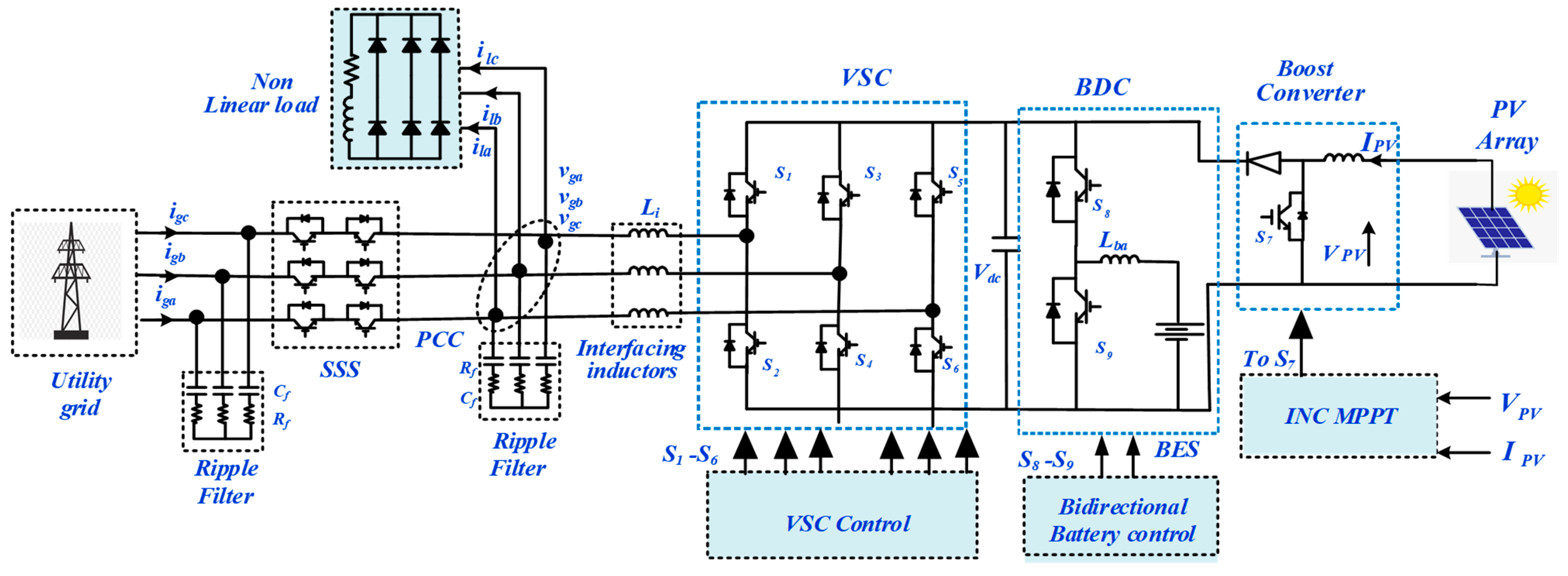
Figure 1 depicts a three-phase grid-connected solar-energy-based microgrid with battery energy storage linked at the VSC’s DC link through a BDC. A BDC connects the battery to the DC connection, reducing battery current ripples. When the grid is not present, the static transfer switch (SSS) controls from grid-connected to standalone mode. The suggested topology provides power to the local loads. Furthermore, the VSC is linked to the PCC by interfacing inductors. These interface inductors are used to decrease VSC current ripples. Furthermore, an RC filter is attached at PCC to prevent VSC voltage switching noise.
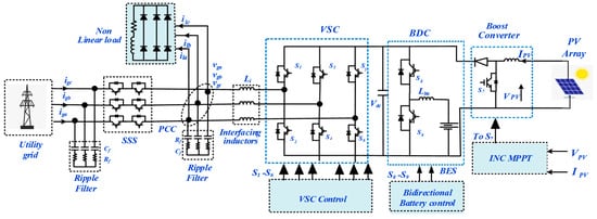
Figure 1.
System topology.
3. Control Algorithm
The control algorithms of the PV-BESS grid-connected microgrid include the following: DC-DC boost converter controller for the MPPT algorithm, GC-sigmoid-function-based LMS for VSC control, standalone-mode control, synchronization control for a smooth transition of GIA mode to SAI mode and vice versa, and BDC control for the battery.
3.1. DC-DC Boost Converter Controller for MPPT Algorithm
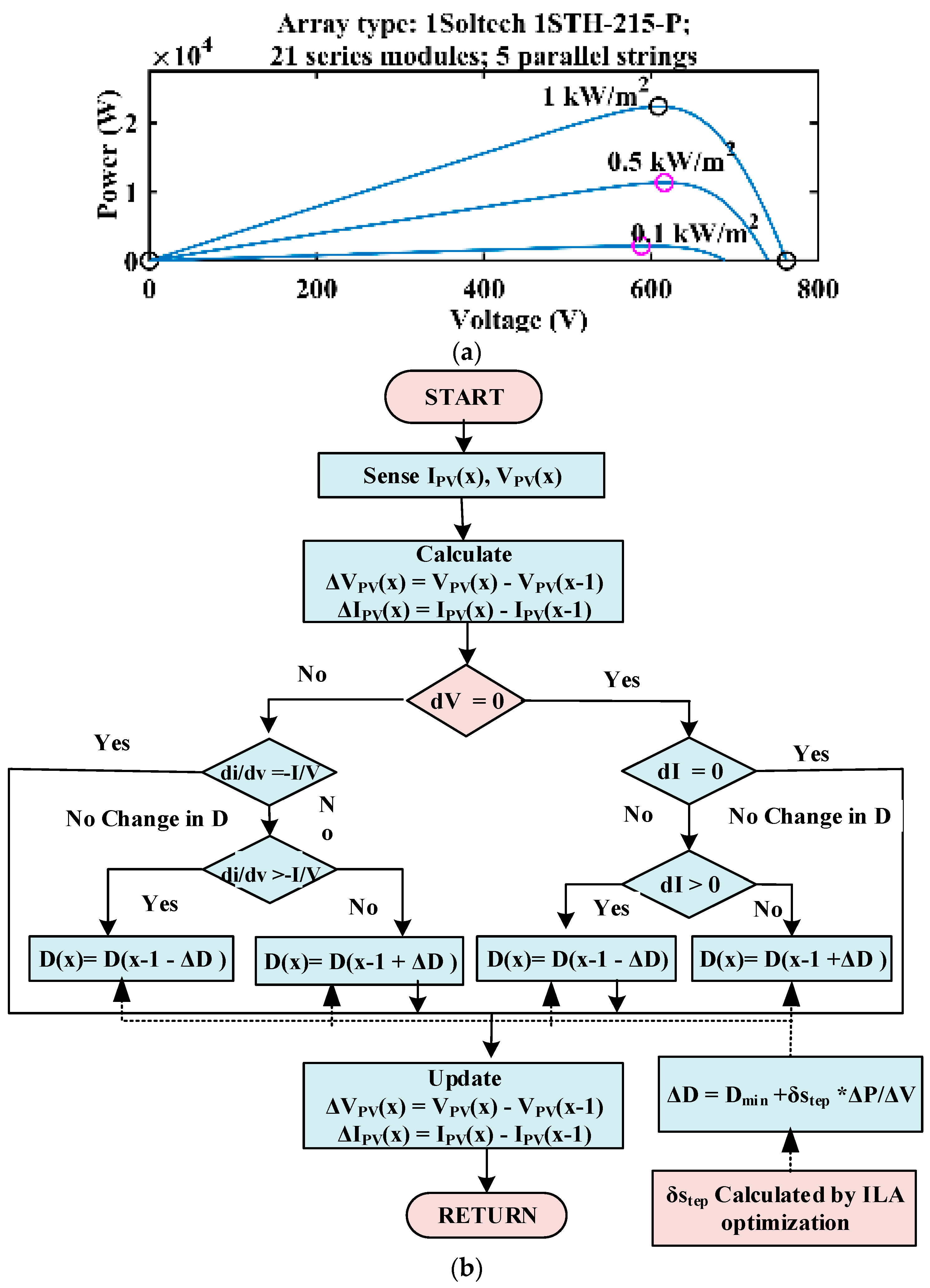
The array voltage is modified using the INC approach in accordance with the MPP. The MPP is calculated by equating the incremental conductance with the instantaneous conductance. When the incremental conductance equals the instantaneous conductance, the MPP is attained. Figure 2a,b shows the solar power curve at different irradiation levels of the solar array used in this work, and Figure 2b gives the algorithm of the INC strategy [7].
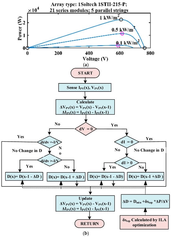
Figure 2.
INC MPPT: (a) power characteristics; (b) flow chart.
3.2. GC-Sigmoid-Function-Based LMS for VSC Control
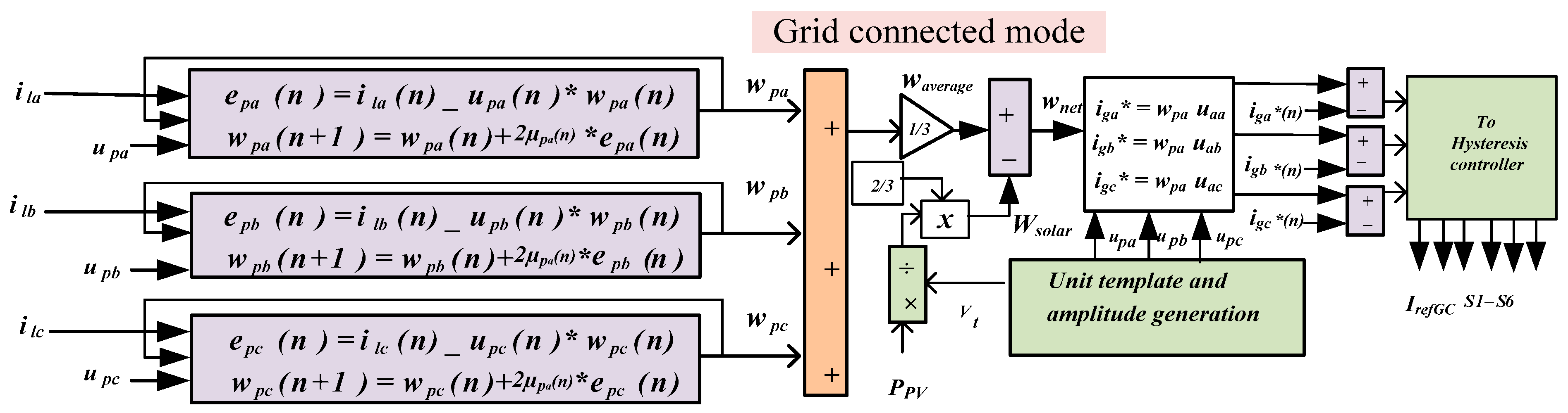
In grid-connected mode, VSC control is used for extracting the fundamental component of the load [26]. The SFB-VSS adaptive method is used to increase convergence speed, accuracy, and anti-noise performance. This method employs a bigger step size in the early stage to attain a higher convergence rate and then maintains a lower step size after basic convergence. The block diagram representation of control for the VSC is shown in Figure 3 and involves the following steps.
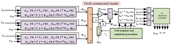
Figure 3.
Grid-connected VSC control.
3.2.1. Terminal Voltage and Unit Template Calculation
The terminal voltage of the grid (Vt) is calculated. The three-phase PCC voltages are estimated as follows:
where are line voltages sensed by the utility. The grid amplitude voltage (Vt) is given by
Unit templates (in phase) are given by
3.2.2. Weight Component Calculation
The active weight component of the load of all three phases (i.e., a, b, and c) is given by the equations shown in Figure 2. The phase a active weight component is calculated using the following equation:
The adaptive algorithm uses an input signal and error signals to update the weighting coefficient of a digital filter, constantly changing the output signal and recalculating the error signal. The nonlinear function of the step factor and the error of the SFB-VSS control are shown in Equation (5) and Figure 3.
and are constant variables. is the genetic coefficient variable () for the control of the convergence rate. To further suppress the disruption of abrupt noise and introduce the estimate of , error autocorrelation may effectively eliminate the influence of independent noise, and it is a good balance near the optimal weights. Instead of the quantity standard, the algorithm uses . Using the same formulas, the weights of the other two phases ( (n) and (n)) can also be estimated.
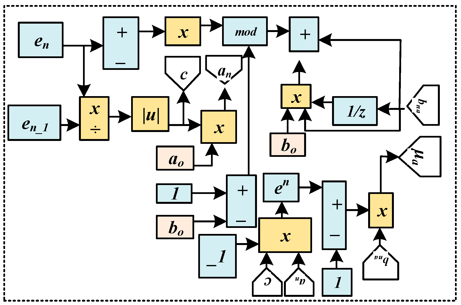
Figure 4 shows the step factor calculation block diagram.
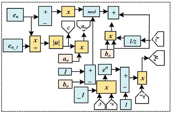
Figure 4.
Nonlinear function of step factor.
and are used to calculate the degree of change in the curve and to determine the change in the range of values of the function, respectively, and are given as
3.2.3. Reference Current Calculation
The reference currents of the three phases are calculated by multiplying the average weight component (waverage) by the corresponding unit template of the phase. The average weight component is calculated using the following equation:
Subtracting the PV component from the average weight gives the net active weight component (Wnet). The solar power feed-forward term is calculated as
The reference currents are obtained by multiplying the net weight component by the estimated in-phase unit templates and are given by
3.2.4. Switching Pulse Generation
The hysteresis current controller (HCC) is used to generate switching pulses. The error signal is calculated by subtracting the grid’s reference current from the sensed grid currents and goes to the HCC for VSC pulse generation.
3.3. SA Mode of VSC Control Operation
The solar PV–battery microgrid operates in standalone mode when the grid is off or there is any grid outage condition in the system. The synchronizing signal of zero is given to SSS, causing the system to operate in the standalone mode of operation. In this mode, VSC control shifts to voltage-controller-based VSC control as shown in Figure 5.
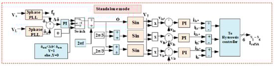
Figure 5.
Standalone-mode control.
The reference load voltages (vla* vlb*, vlc*) are calculated as
where ws is the reference voltage frequency. These reference load voltages are compared to the actual sensed load voltage, and the error is fed to the PI controller. This PI controller will give reference load currents which are then compared with the actual sensed load voltage, and the error is given to HCC for the generation of switching pulses in the SA mode of operation.
3.4. Synchronization Control
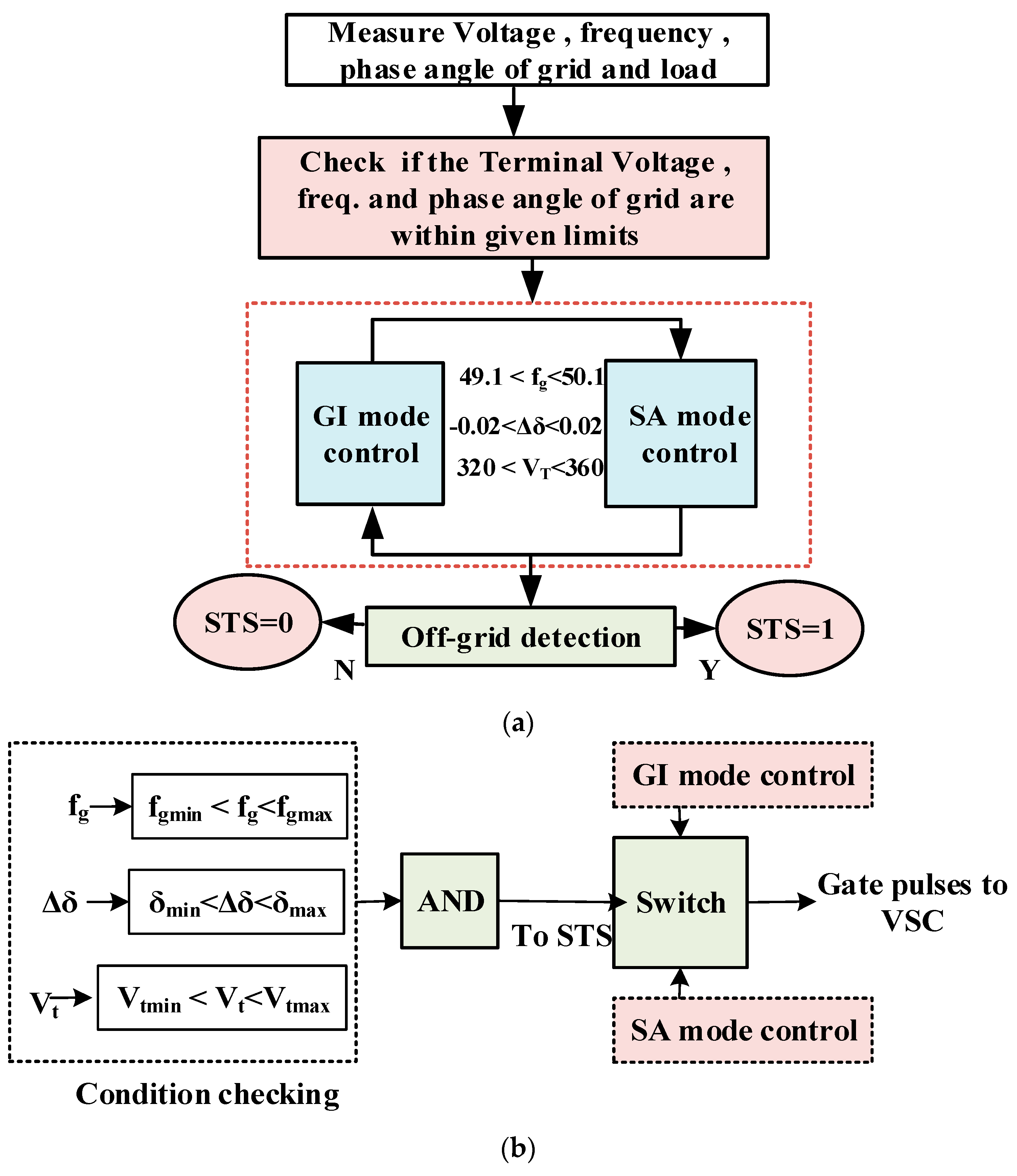
The synchronization controller’s block diagram is shown in Figure 6a,b. Before resynchronization, the grid voltage magnitude and frequency and the difference between the grid voltage phase and load voltage should be within the specified limits. When all of the requirements are met, the synchronization signal is generated (1), the SSS closes, and the system operating mode is changed from SA mode to GC mode. However, when the condition is false, the synchronization signal is false (0), the SSS opens, and the system operates in the SA mode of operation.

Figure 6.
Synchronization controller: (a) flow chart; (b) synchronization conditions.
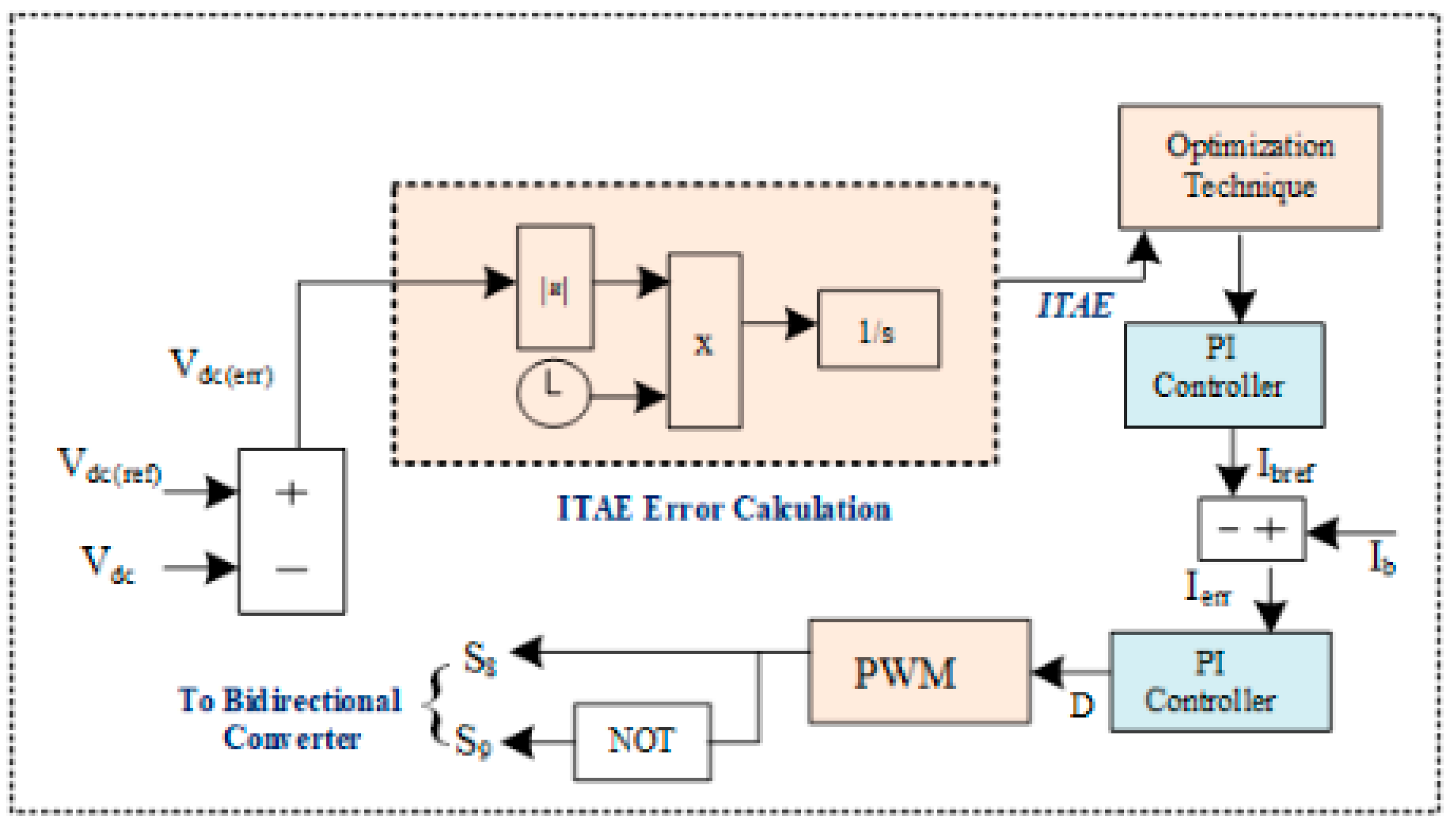
3.5. ILA-Based BDC Control
The battery energy storage maintains a constant reference voltage (Vdcref) across the DC-link capacitor by managing the BDC gating sequences. The control block diagram of the BDC is shown in Figure 7. The difference between the Vdcref and the sensed DC-link voltage (Vdc) is supplied to the PI controller. The PI controller produces the Ibref (reference battery current), which is compared with the sensed battery current. The error is fed to the PI controller, and the output is given to the PWM generator for generating switching pulses to the BDC.
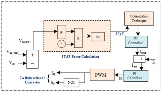
Figure 7.
ILA-optimization-based DC-link voltage control.
To enhance the PI controller, GA, PSO, and ILA optimization are used to calculate the gains. The optimized values enhance the DC bus voltage stability, thereby reducing the Vdcerr and enhancing the battery current as well. ILA-optimization-based gain values enhance the system more as compared with other manual and optimized values. Table 1 gives the PI controller parameters obtained using various optimization techniques.

Table 1.
PI controller parameters.
ILA Optimization
The Incomprehensible but Intelligible-in-time (IbI) logics technique (ILA) is a novel optimization technique based on IbI logics theory [27]. Even sophisticated machines cannot perform all of the brain’s computations in one second since the human mind is a complicated biological member with distinctive abilities. The ILA algorithm is based on this behavior. What it has not learned is a non-logic from a mental viewpoint and in accordance with human knowledge. This, however, can change with time. At the same time, the IbI logic is a non-logic which might one day become obvious logic. Exploring, integrating, and exploiting are the three steps of the ILA. Any of the three ILA phases serves a specific purpose. The exploration phase has the role of identifying new solutions in the search space. The integration phase is responsible for combining the new and old solutions. The exploitation phase is in the midst of discovering the optimal solution in the search space. Several benefits distinguish the ILA from other optimization techniques. First, the ILA may individually monitor the exploration and exploitation stages. This allows the user to control the algorithm’s performance and alter its parameters as needed. Second, the ILA is incredibly effective at determining the optimal solution. Third, the ILA’s computation time is low.
ILA optimization is subdivided into many stages; the first is the preparation phase, which is followed by the other three stages. Each phase has a distinct function. When one step is completed, the solutions advance to the next phase, with no way back to the current iterations. Table 2 provides the different variables used for ILA optimization.
Table 2.
ILA Parameters.
- Preparation phase
The proposed algorithm involves a preparation phase and stage 1 of optimization. The initial values of ILA parameters are specified, and the number of iterations for each of the nm models is determined by tm and is given by
tm = nt+1/nm
nt+1 = ps1 × NT
Each model is optimized tm times, with the final findings being transmitted to the next model and optimized tm times more. After the iterations for the first stage are completed, all the findings are included in stage 2.
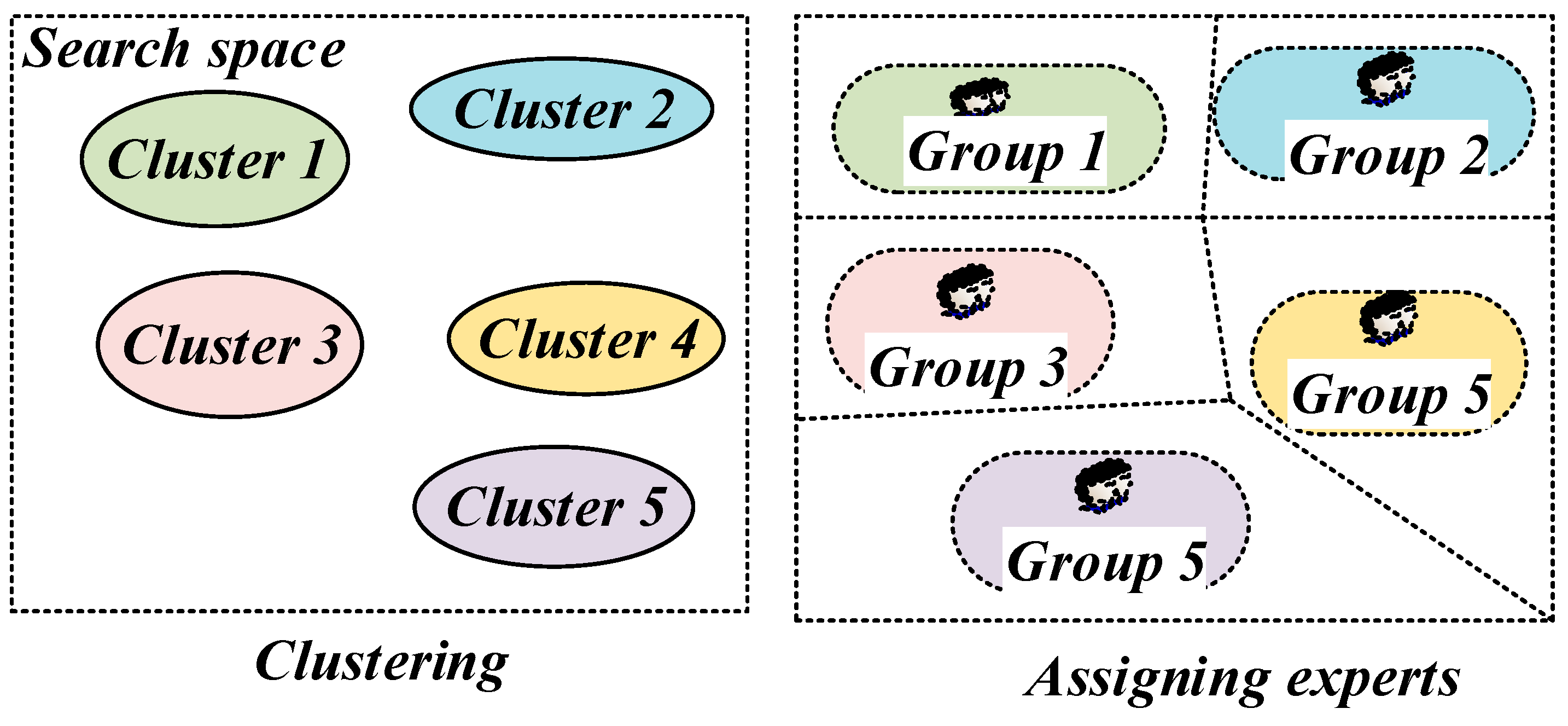
The k-means clustering technique is used before initiating the process of optimization to divide experts into groupings determined by their knowledge. The total number of groups in every model is chosen at random using the randi function and is given by
ng,m = randi (ng,max) m = 1,2, … nm.
If the number of needed clusters is less than ng,m, Equation (18) is ignored, and the prior model’s clusters are allocated to the current model. Following clustering, each expert is allocated to one of the groups, and the defined groups are transferred to stage 1 for optimization, as shown in Figure 8.

Figure 8.
Grouping of experts.
- Stage 1: Group work
Each group concentrates on an individual section of the possible solutions in the first stage of the process and tries to identify the best NL in that section. Experts (Ei) use their group’s expertise to increase their starting fitness (NL) in tm iterations. For each of the experts, three parameters are chosen: the best NL value in the iteration before it (Ei,p), the best expert in each group (Ei,g), and an average of the Es achieved by every group in the iteration that follows.
For each nNL expert, Equations (19)–(21) are used to calculate three different parameters of the IbI logic, namely Ci, Di, and Pi, which indicate the ith expert’s comprehensibility, degree, and probability, respectively.
A normalizing approach is used to minimize the amounts between 0 and 1 in order to make use of the values generated from Equations (19) and (20). Rc,i, RD,i, and RP,i are the degree, comprehensibility, and probability ratios proposed by Equations (22)–(24). In stage 1, these ratios are altered at the beginning of each iteration.
The first task is to calculate new knowledge, K0,S1 and K1,S1. The parameters BP, BC, and BD are chosen randomly between Bmin and Bmax in each iteration If an Ei is near the logic of the present iteration, it can be kept in the calculations since it could enhance in adhering iterations. The process of determining the K0,S1 is illustrated in Figure 9.
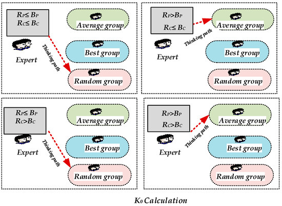
Figure 9.
Knowledge (K0) calculation.
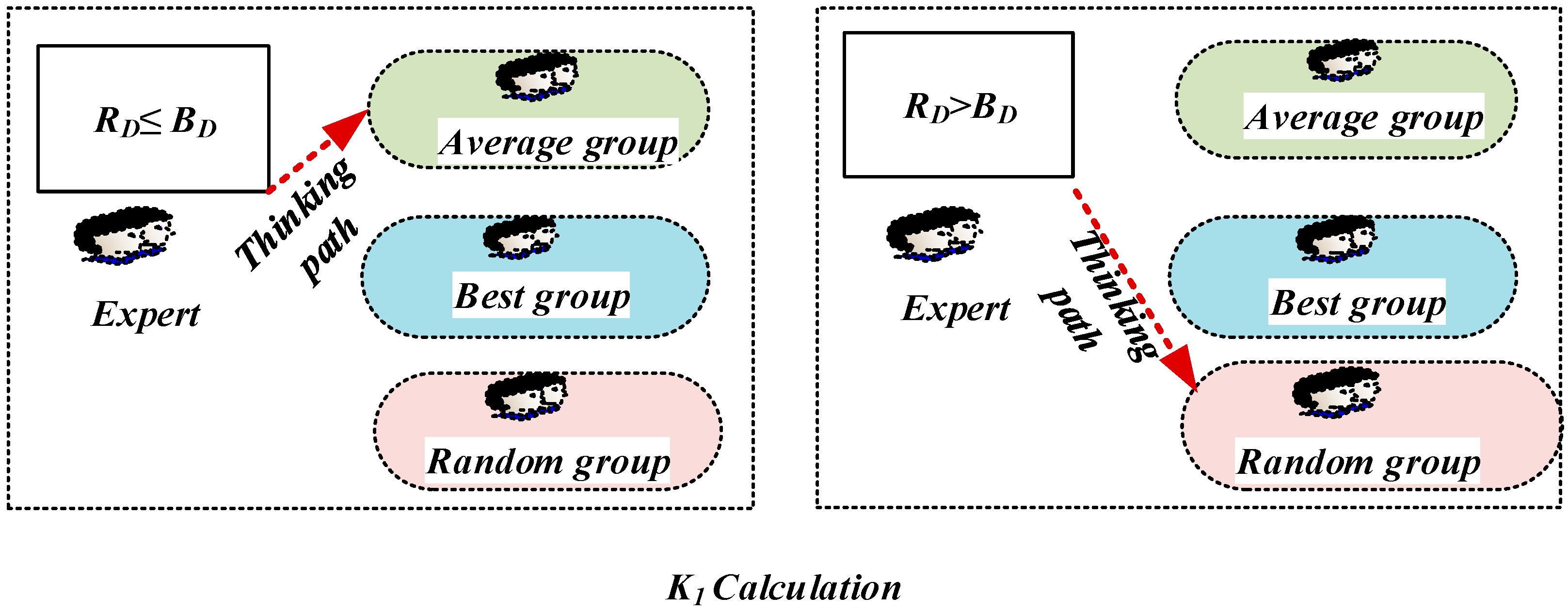
Based on the data that are accessible, the distance parameter RD,i serves to supply new knowledge to the ith expert Ei.
When a member’s distance from its prior value is more than BD, an attempt is made to improve the condition for this expert as shown in Figure 10. In other circumstances, new knowledge (random scenario) can be used with Equation (25).
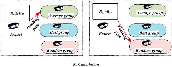
Figure 10.
Knowledge (K1) calculation.
The overall knowledge is given by
The amount of Ei is affected by Equation (27), and a secondary update is given by
The best value (min.) of E is given by
The fitness function is named f, based on Equation (30), the new value is compared to the prior value, and the expert retains the situation having the highest level of fitness, as shown in Figure 11.
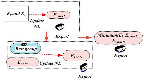
Figure 11.
Calculation of final NL in stage 1.
After stage 1 is finished, the final solutions are transferred to stage 2 for integration.
- Stage 2: Integration
In the second stage of the algorithm, all experts are integrated and use the knowledge provided in the current iteration to improve their NL value. The ratios of RC and RD are determined using Equations (22) and (23), with the best solution, EI, being used to calculate RP. Each iteration applies new knowledge (KS,2) to each expert, with coefficients c5 and c6 adhering to random experts from the total population and the experts’ average, respectively and is shown in Figure 11. Equation (31) is used to determine the final knowledge based on KS2, with c6 indicating a random vector between −0.75 and 0.75.
Equation (30) determines the initial update based on the value received from Equation (29) and the best expert’s current knowledge, EI. When the aim is the minimal value of the fitness function, the ultimate scenario for Ei is the outcome of Equations (32) and (33).
The coefficient c7 has a value from −0.75 to 0.75, and for c8, from 0 to 1 is selected.
- Stage 3: IBL logic search
The suggested method focuses on enhancing each member’s expertise by using the average collective knowledge of all experts. It then performs a secondary update on each researcher’s knowledge. The process is performed nt3 times more until the stop requirements are met. The average of previous knowledge is determined at the start of each iteration. Equations (35)–(39) specify the value of KS3, and the value of ES3,i is determined based on the fitness function’s goal.
For optimizing the minimization function Equation (15), the number of iterations was first taken as 5; then, for better results, it was taken as 30, and the population number was 50. The convergence curve of the implemented optimization is shown in Figure 12.
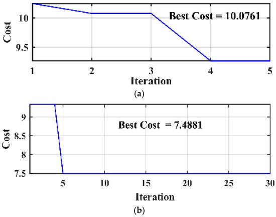
Figure 12.
Convergence curve: (a) 5 iterations; (b) 30 iterations.
4. Simulation Results
In the MATLAB/Simulink environment, the proposed grid-connected PV-BS-based AC microgrid was simulated. The responses are shown in both GI mode and SAI mode under varied dynamic and steady-state conditions.
4.1. Steady-State Response of the System
Figure 13 shows the steady-state response of the system in the GC mode of operation. vg (V) and ig (A) represent grid voltage and current, il and ivsc are the load and compensation current, Vt and Vdc are the terminal and DC-link voltages, and Ibat and IPV are the battery and photovoltaic currents at 1000 W/m2. Figure 13a shows that under steady-state conditions, the grid current and voltage remain sinusoidal and balanced. Vt and Vdc are constant and within limits. The system’s THD remains satisfactory as per IEEE standard 519. Figure 13b shows that the proposed control improves power quality.
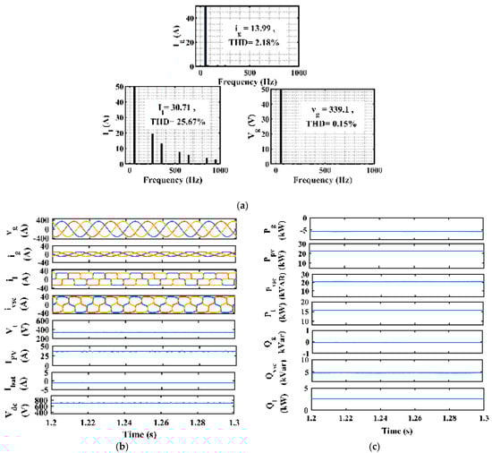
Figure 13.
(a) THD analysis (Ig, Il, Vg); (b) vg, ig, Il, ivsc, IPV, Ibat, and Vdc; (c) Pg, Ppv, Pvsc, Pl, Ql, Qvsc, and Ql.
Figure 13c shows the grid’s real and reactive power (Pg, Qg), the solar power (Ppv), the compensating real and reactive power (Pvsc, Qvsc), and the load’s real and reactive power (Pl, Ql). The results show that Ppv and Pg supply power to the load. The reactive power supplied to the grid is 0. In steady-state conditions, the extra power is given to the grid. The load is mostly met by the renewable-energy-based source, i.e., Ppv, which puts less burden on the conventional grid. The extra power is given to the battery for its charging. The Vdc remains constant, which enhances the system’s stability.
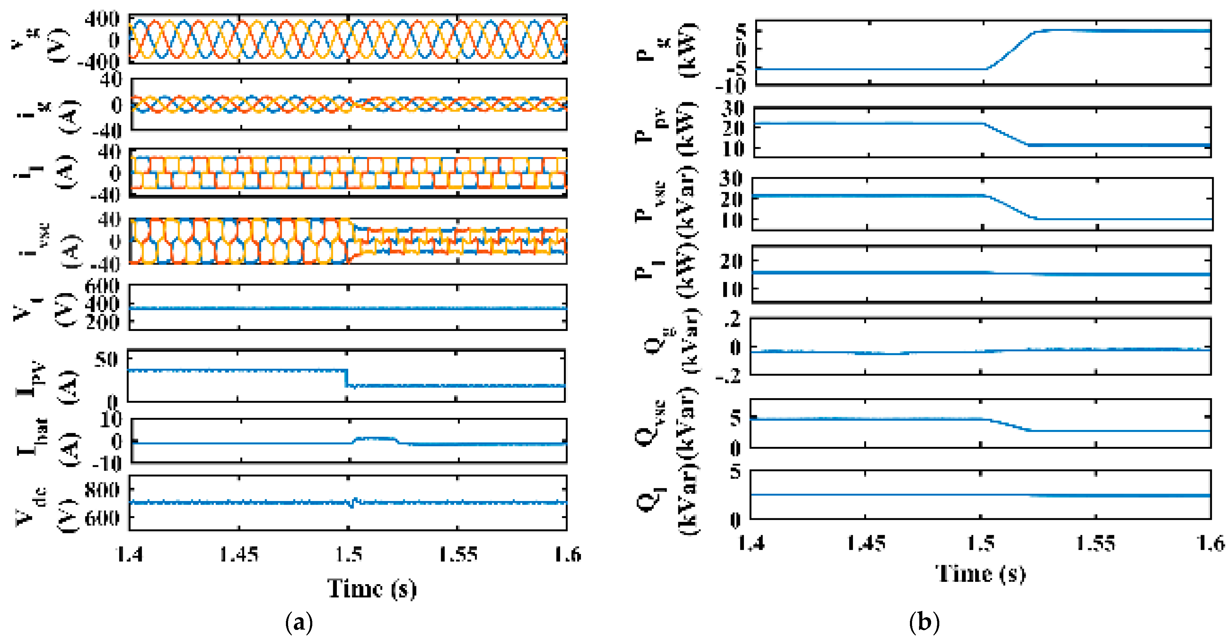
4.2. Dynamic Response under Balanced Nonlinear Load and Change in Solar Irradiation
Figure 14a represents the dynamic response of the system. The solar radiation is altered from 1000 W/m2 to 500 W/m2 at 1.5 s as shown. Due to the decrease in solar generation, the grid has to supply surplus power, so ig (A) increases as shown. vg (V) and ig (A) remain sinusoidal and balanced irrespective of dynamic conditions. il remains constant but ivsc decreases as Ipv decreases, whereas Ibat increases, showing a decrease in solar current and the discharging of the battery. Vt and Vdc also remain steady, showing they are less affected by solar irradiation variation. Figure 14b shows that Pg is increased due to a decrease in Ppv, showing that the grid is supplying the deficit to reach constant load power Pl. The proposed system ensures system stability and power balance in the dynamic conditions of a renewable-energy-based MG.

Figure 14.
Dynamic response under irradiation change: (a) vg, ig, il, ivsc, IPV, Ibat, and Vdc; (b) Pg, Ppv, Pvsc, Pl, Ql, Qvsc, and Ql.
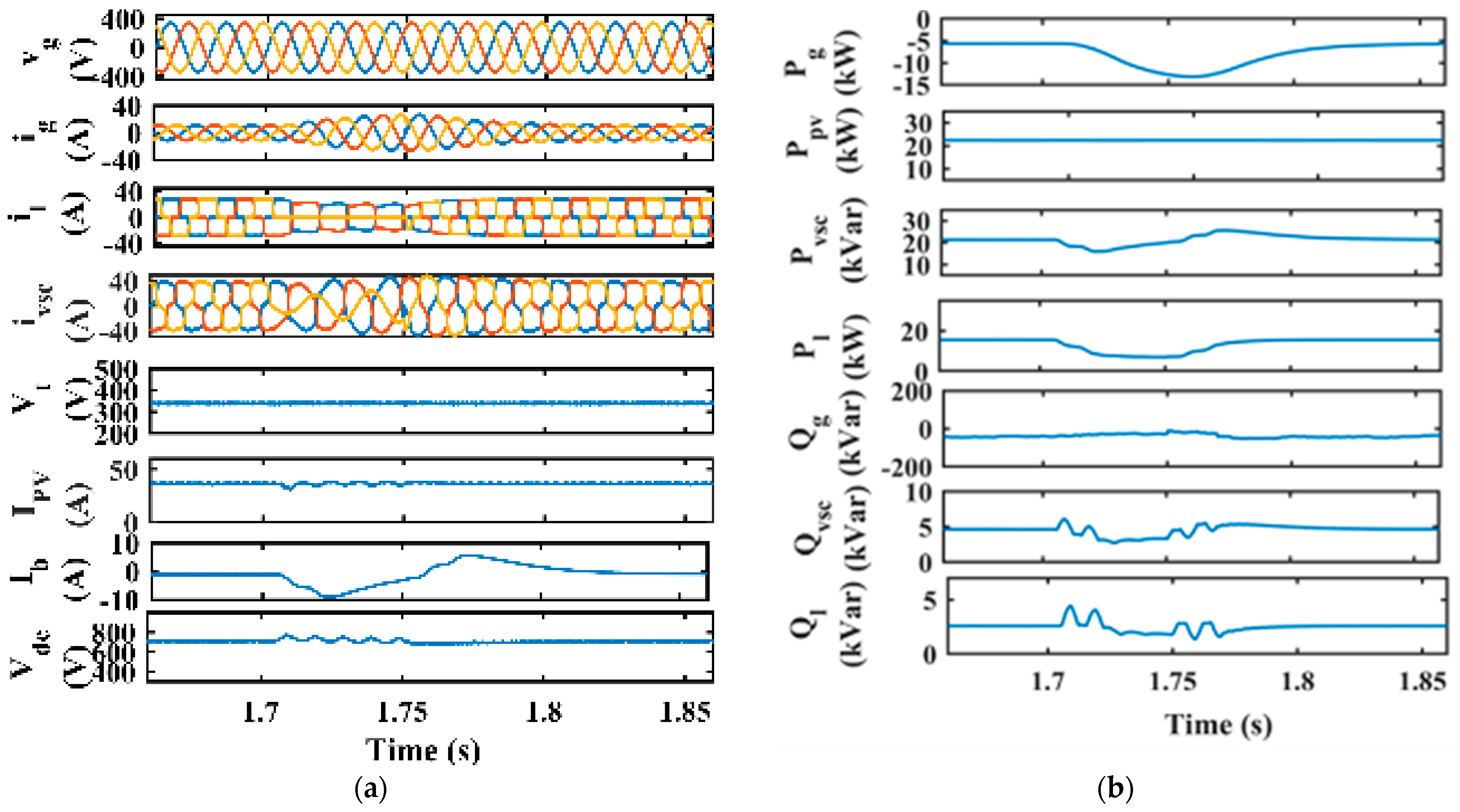
4.3. Dynamic Response under Unbalanced Nonlinear Load and Constant Solar Irradiation
Figure 15a represents the dynamic response of the system under load unbalance. The solar radiation is kept constant at 1000 W/m2. Load unbalance is introduced by removing the load in one of the phases at 1.7 s to 1.75 s as shown. The load unbalance disturbs the system as ig (A) increases and vg (V) remains constant, and both remain in phase and balanced. When the load is reconnected, the system shifts back to steady-state conditions. Vdc and Vt show fewer fluctuations, whereas Ibat shows deviation due to the abrupt charging of the battery due to a sudden decrease in load. Figure 15b shows the dynamic response of the power of the load grid and VSC compensator. The results show that Pl decreases during load unbalance, and extra power from Ppv is given to the grid.
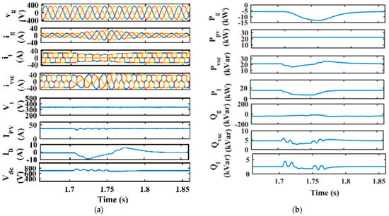
Figure 15.
Dynamic response under load unbalance: (a) vg, ig, il, ivsc, IPV, Ibat, and Vdc; (b) Pg, Ppv, Pvsc, Pl, Ql, Qvsc, and Ql.
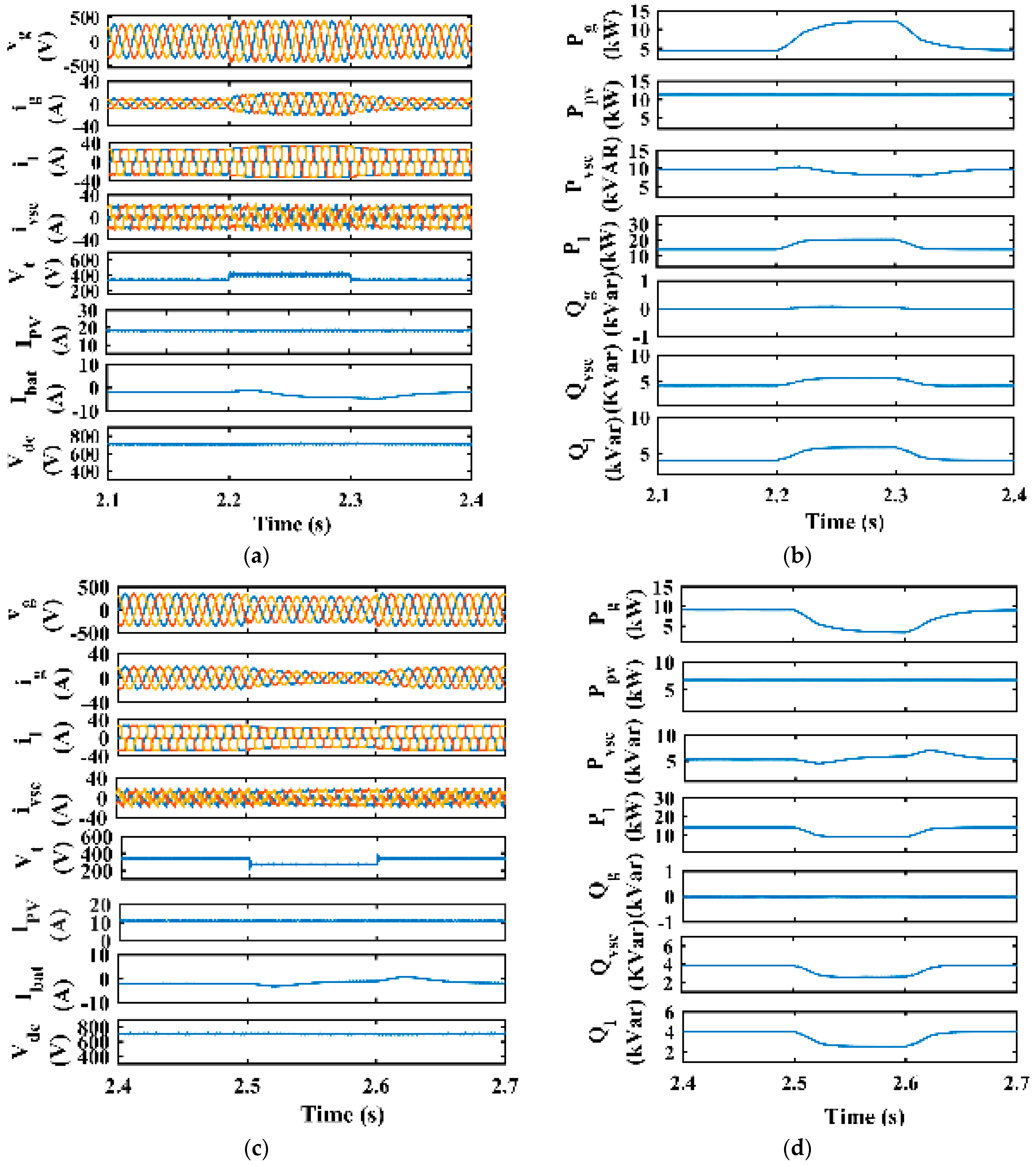
4.4. Dynamic Response under Abnormal Voltage Conditions
Figure 16a–d represent the dynamic response of the system under abnormal grid voltage conditions (grid voltage sag and swell). Figure 16a shows the voltage swell created by increasing the grid voltage from 1 p. u to 1.2 p. u at 2.2 s to 2.3 s of the simulation time. Irrespective of the increase in voltage, the control ensures that both vg (V) and ig (A) remain balanced and sinusoidal. Due to the rise in grid voltage, Vt (V) increases. The PV side remains unaffected as Ipv (A) remains constant. The battery is in a charged state, as depicted by Ibat (A). Vdc (V) remains constant irrespective of the change in grid voltage. Figure 16b shows the power balance; grid power increases from 2.2 s to 2.3 s and comes back to a steady state after the disturbance is cleared. Ppv (kW) and Pl (kW) remain constant while Qg (kVar) remains constant, showing there is no exchange of reactive power to the grid. Figure 16c shows the voltage sag created by decreasing the grid voltage from 1 p. u to 0.8 p. u at 2.5 s to 2.36 s. Despite the decrease in voltage, the control ensures that both vg (V) and ig (A) remain balanced and sinusoidal. Due to the fall in grid voltage, Vt (V) decreases, and the PV side remains unaffected. The battery is in a charged state, as depicted by Ibat(A). Vdc (V) remains constant irrespective of the decrease in grid voltage. Figure 16d shows the power balance.
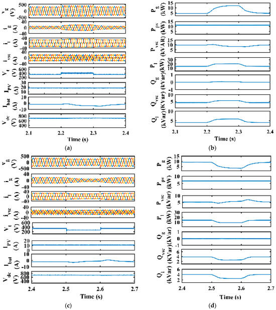
Figure 16.
Dynamic response under grid voltage abnormalities: (a) vg, ig, il, ivsc, IPV, Ibat, and Vdc; (b) Pg, Ppv, Pvsc, Pl, Ql, Qvsc, and Ql; (c) vg, ig, Il, ivsc, IPV, Ibat, and Vdc; (d) Pg, Ppv, Pvsc, Pl, Ql, Qvsc, and Ql.
The power decreases from 2.5 s to 2.6 s and comes back to a steady state after the disturbance is cleared. Ppv and Pl remain constant while Qg remains constant, showing there is no exchange of reactive power to the grid.
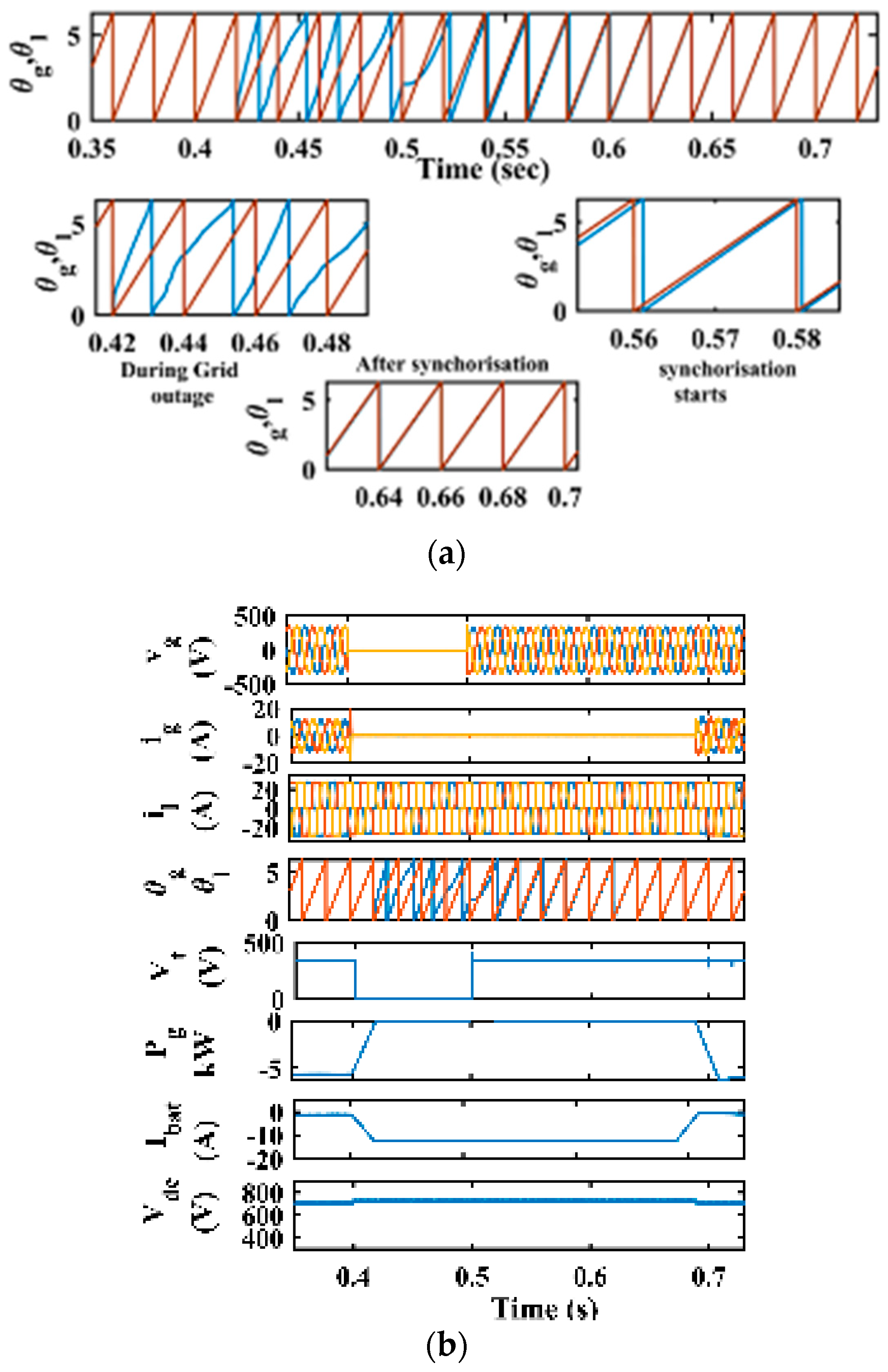
4.5. Seamless Mode Transfer
Figure 17a,b represent the seamless mode transfer from SI mode to GC mode. The grid is removed at 0.4 s, and the grid is synchronized back at 0.5 s. During islanding, Vt (V), the phase angle of the grid (θg), and the grid frequency (fg) deviate. Vt (V) is maintained at the desired level after the grid is reconnected by the synchronization controller, as shown in Figure 17a. The Vdc is maintained constant. θg and the phase angle of the load θl are synchronized, as shown in Figure 17b.

Figure 17.
Response of system during mode change: (a) θg and θl; (b) vg, ig, il, θg, θl, Vt, Pg, Ibat, and Vdc.
4.6. Comparative Analysis of DC-Link Voltage and Battery Current
Figure 18a,b represent the comparative analysis of the DC-link voltage and battery current. The BDC PI controller gains are optimized by using different optimization techniques, i.e., GA, PSO, manual tuning, and ILA optimization given in Table 1. Figure 18a shows that the DC-link voltage has fewer fluctuations and has less impact during the dynamic response of the system for the gains of the ILA-optimized PI controller. The steady-state and dynamic responses show that ILA-optimized gains give better stability, fewer oscillations, and hence, lesser values of interfacing capacitance. Table 3 shows that the relative percentage error of Vdc is less for the ILA-based PI controller when the reference value of Vdc is 700 V.
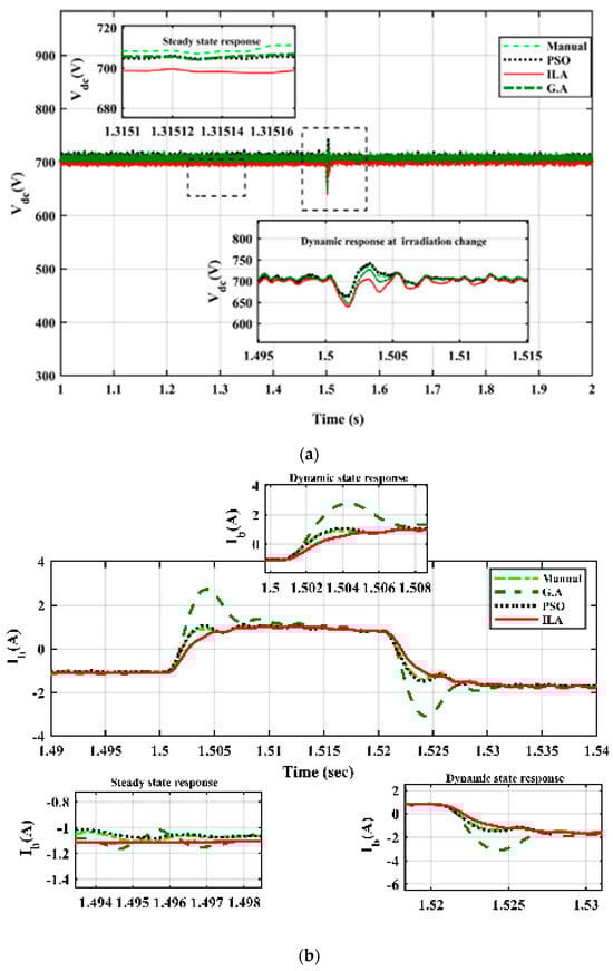
Figure 18.
Comparative analysis: (a) Vdc; (b) Ibat.
Table 3.
Relative percentage error of Vdc (V).
Figure 18b shows the dynamic and steady-state responses of the battery at different optimized values. The ILA-optimized gains enhance the battery performance by reducing the fluctuations in the battery current and thus enhancing the reference battery voltage (ibref). This enhances the control for the generation of switching pulses to the BDC.
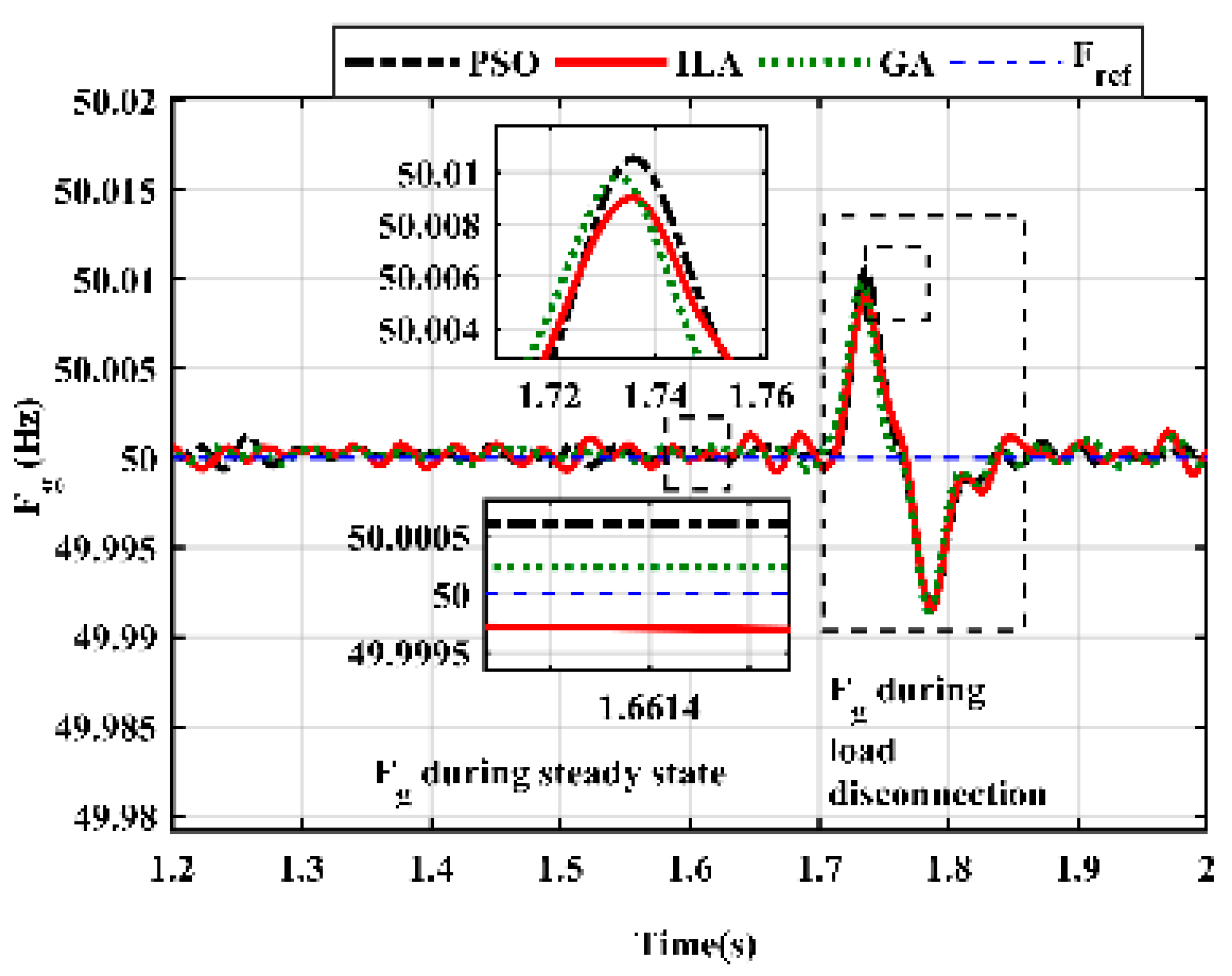
4.7. Comparative Analysis of Grid Frequency
Figure 19 shows the comparative analysis of grid frequency under steady and transient conditions. The load is removed at 1.7 s and connected back at 1.75 s. The optimized parameters also enhance the grid frequency. The ILA-optimized PI controller enhances the stability. The Fg remains within limits (50 Hz) irrespective of load disconnection, and the steady-state response is also satisfactory.
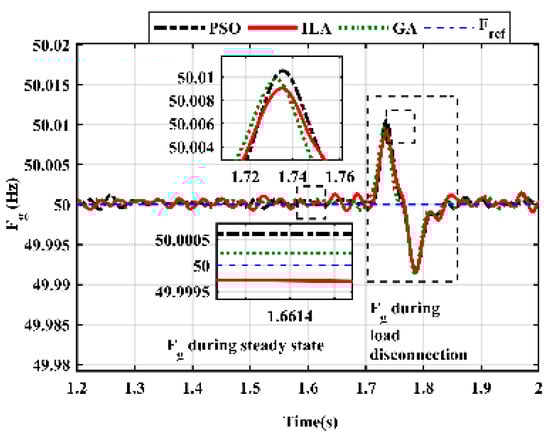
Figure 19.
Comparative analysis of frequency.
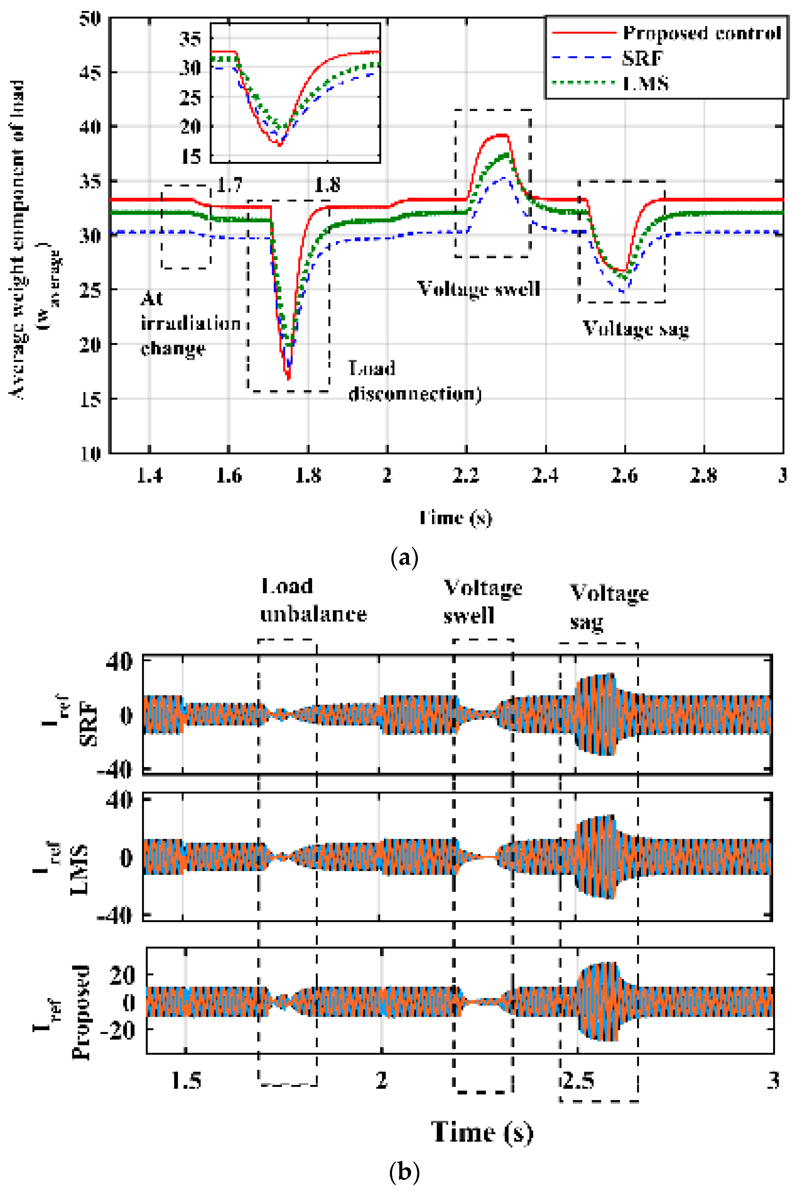
4.8. Comparative Analysis of Proposed VSC Control with Conventional LMS and SRFT Control Algorithms
Figure 20a shows the estimated average active weight of the load current generated by LMS, SRF, and the proposed SFB-VSS adaptive method (Waverage). All algorithms produce sinusoidal current under load unbalance. Various dynamic conditions include solar irradiation change, load unbalance, voltage sag, and voltage swell. The proposed control produces a better active weight component of the load as compared to other algorithms. The proposed LMS has fast convergence and low oscillations as compared to conventional SRF and LMS control, as shown. SFB-VSS-LMS has better noise and DC offset rejection capability. Figure 20b shows the sinusoidal current generated by using different control algorithms. The comparative analysis shows that the sinusoidal current generated by the proposed control is closer to the reference value of the grid current.
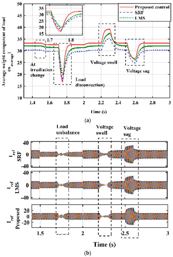
Figure 20.
Comparative analysis: (a) SFB-VSS-LMS-based VSC control; (b) generated sinusoidal current.
5. Conclusions
In this paper, a grid-connected three-phase microgrid has been presented. The optimal design and control of VSC control for both the grid-connected and standalone modes of operation have been shown for this topology. The battery performance has been increased by the optimal design of BDC control by using the ILA-optimization-based gains of the PI controller. The battery current has fewer fluctuations and shows smooth charging and discharging of the battery, enhancing the life of the battery. The optimized gains enhanced the Vdc voltage by reducing the relative percentage error from the reference value. The relative percentage error of Vdc is only 0.5714% as compared to the PI gains obtained from GA, PSO, and manually tuned gains. Power balance has been achieved in all steady-state and dynamic conditions like load unbalance, irradiation change, and grid voltage dynamics. During grid islanding and resynchronization, the synchronization controller allows for a smooth transition of VSC control from GA mode to SA mode. The synchronization controller checks all three conditions i.e., grid frequency, terminal voltage, and the phase angle of the grid. When the grid is not available for any reason, the system has the capability to work in isolated mode as well. Also, the proposed control maintains the frequency of the grid within the standard limits in all dynamic conditions. Under dynamic situations, the system performs well, with a THD of around 5%, i.e., as per IEEE standard 519 [28]. The proposed control SFB-VSS-LMS was compared with SRF and LMS control. The comparison shows that the oscillations in the weight component are fewer as compared with those in SRF and LMS control. The convergence rate of the system has also been improved, and the control provides better DC offset rejection. The proposed system was simulated in MATLAB Simulink, and all the optimizations were carried out offline.
Author Contributions
Conceptualization, F.A.S. and I.H.; methodology, F.A.S.; software, F.A.S.; validation, F.A.S., I.H. and S.J.I.; investigation, I.H.; data curation, F.A.S.; writing—original draft preparation, F.A.S.; writing—review and editing, F.A.S.; visualization, I.H. and S.J.I.; supervision and project administration, I.H.; funding acquisition, I.H. All authors have read and agreed to the published version of the manuscript.
Funding
This research received no external funding.
Data Availability Statement
Not applicable.
Conflicts of Interest
The authors declare that they have no conflict of interest.
Abbreviations
PV array parameters: IMPP = 7.35, VMPP = 29, VPV = 580, IPV = 21.42, PPV(max) = 22 kW, ns = 21, np = 5, boost converter Lboost = 2 mH; battery: 700 V, 100 Ah, Li = 3 mH; grid parameters: Vll = 415 V f = 50 Hz, Rf = 5 Ohm, Cf = 10 × 10−6; DC-link voltage: 700 V; synchronization limits: 0.02 < Δδ < 0.02, 49.1 < fg < 50.1, 320 < Vt < 360; switching frequency: 10 kHz.
References
- Pali, B.S.; Vadhera, S. Renewable energy systems for generating electric power: A review. In Proceedings of the 2016 IEEE 1st International Conference on Power Electronics, Intelligent Control and Energy Systems (ICPEICES), Delhi, India, 4–6 July 2016. [Google Scholar]
- Tkac, M.; Kajanova, M.; Bracinik, P. A Review of Advanced Control Strategies of Microgrids with Charging Stations. Energies 2023, 16, 6692. [Google Scholar] [CrossRef]
- Li, B. Build 100% renewable energy based power station and microgrid clusters through hydrogen-centric storage systems. In Proceedings of the 2020 4th International Conference on HVDC (HVDC), Xi’an, China, 6–9 November 2020; pp. 1253–1257. [Google Scholar]
- Escobar-Orozco, L.F.; Gómez-Luna, E.; Marlés-Sáenz, E. Identification and Analysis of Technical Impacts in the Electric Power System Due to the Integration of Microgrids. Energies 2023, 16, 6412. [Google Scholar] [CrossRef]
- Hirsch, A.; Parag, Y.; Guerrero, J. Microgrids: A review of technologies, key drivers, and outstanding issues. Renew. Sustain. Energy Rev. 2018, 90, 402–411. [Google Scholar] [CrossRef]
- Mishra, J.; Das, S.; Kumar, D.; Pattnaik, M. Performance Comparison of PO and INC MPPT Algorithm for a Stand-alone PV System. In Proceedings of the 2019 Innovations in Power and Advanced Computing Technologies (i-PACT), Vellore, India, 22–23 March 2019; pp. 1–5. [Google Scholar]
- Abouobaida, H.; Mchaouar, Y.; Abouelmahjoub, Y.; Mahmoudi, H.; Abbou, A.; Jamil, M. Performance optimization of the INC-COND fuzzy MPPT based on a variable step for photovoltaic systems. Optik 2023, 278, 170657. [Google Scholar] [CrossRef]
- Srinivas, V.L.; Singh, B.; Mishra, S. Fault ride-Through strategy for two-stage grid-connected photovoltaic system enabling load compensation capabilities. IEEE Trans. Ind. Electron. 2019, 66, 8913–8924. [Google Scholar] [CrossRef]
- Debnath, D.; Chatterjee, K. Two-Stage Solar Photovoltaic-Based Stand-Alone Scheme Having Battery as Energy Storage Element for Rural Deployment. IEEE Trans. Ind. Electron. 2015, 62, 4148–4157. [Google Scholar] [CrossRef]
- Zhao, X.; Yang, Y.; Qin, M.; Xu, Q. ScienceDirect Multi-objective optimization of distribution network considering battery charging and swapping station. Energy Rep. 2023, 9, 1282–1290. [Google Scholar] [CrossRef]
- Chebabhi, A.; Tegani, I.; Djoubair, A.; Kraa, O. Optimal design and sizing of renewable energies in microgrids based on financial considerations a case study of Biskra, Algeria. Energy Convers. Manag. 2023, 291, 117270. [Google Scholar] [CrossRef]
- Choudhury, S.; Varghese, G.T.; Mohanty, S.; Kolluru, V.R.; Bajaj, M.; Blazek, V.; Prokop, L.; Misak, S. Energy management and power quality improvement of microgrid system through modified water wave optimization. Energy Rep. 2023, 9, 6020–6041. [Google Scholar] [CrossRef]
- Okwako, O.E.; Lin, Z.-H.; Xin, M.; Premkumar, K.; Rodgers, A.J. Neural Network Controlled Solar PV Battery Powered Unified Power Quality Conditioner for Grid Connected Operation. Energies 2022, 15, 6825. [Google Scholar] [CrossRef]
- Narayanan, V.; Kewat, S.; Singh, B. Solar PV-BES Based Microgrid System with Multifunctional VSC. IEEE Trans. Ind. Appl. 2020, 56, 2957–2967. [Google Scholar] [CrossRef]
- Gajjar, N.A.; Zaveri, T.; Zaveri, N. Adaptive Ɩ0-LMS based algorithm for solution of power quality problems in PV-STATCOM based system. Bull. Electr. Eng. Inform. 2023, 12, 608–618. [Google Scholar] [CrossRef]
- Dey, D.; Subudhi, B. A Normalized Least Means Absolute Third-Based Adaptive Control Algorithm Design for Grid-Connected PV System. IEEE J. Emerg. Sel. Top. Power Electron. 2023, 11, 2291–2299. [Google Scholar] [CrossRef]
- Kumar, A.; Narayanan, V.; Singh, B. Normalized LMF and CC-ROGI-FLL Techniques for Seamless Synchronization of Double Stage SPV-BES Based Microgrid to Utility Grid. In Proceedings of the 2022 IEEE 2nd International Conference on Sustainable Energy and Future Electric Transportation (SeFeT), Hyderabad, India, 4–6 August 2022; pp. 4–6. [Google Scholar]
- Nazir, F.U.; Kumar, N.; Pal, B.C.; Singh, B.; Panigrahi, B.K. Enhanced SOGI Controller for Weak Grid Integrated Solar PV System. IEEE Trans. Energy Convers. 2020, 35, 1208–1217. [Google Scholar] [CrossRef]
- Srinivas, M.; Hussain, I.; Singh, B. Combined LMS-LMF-Based Control Algorithm of DSTATCOM for Power Quality Enhancement in Distribution System. IEEE Trans. Ind. Electron. 2016, 63, 4160–4168. [Google Scholar] [CrossRef]
- Shatakshi; Singh, B.; Mishra, S. Economic operation of PV-DG-battery based microgrid with seamless dual mode control. In Proceedings of the IECON 2018—44th Annual Conference of the IEEE Industrial Electronics Society, Washington, DC, USA, 21–23 October 2018; pp. 1771–1776. [Google Scholar]
- Rezkallah, M.; Singh, S.; Singh, B.; Chandra, A.; Ibrahim, H.; Ghandour, M. Implementation of Two-Level Coordinated Control for Seamless Transfer in Standalone Microgrid. IEEE Trans. Ind. Appl. 2021, 57, 1057–1068. [Google Scholar] [CrossRef]
- Chankaya, M.; Hussain, I.; Malik, H.; Ahmad, A.; Alotaibi, M.A.; Márquez, F.P.G. Seamless Capable PV Power Generation System without Battery Storage for Rural Residential Load. Electronics 2022, 11, 2413. [Google Scholar] [CrossRef]
- Dhar, R.K.; Merabet, A.; Bakir, H.; Ghias, A.M.Y.M. Implementation of Water Cycle Optimization for Parametric Tuning of PI Controllers in Solar PV and Battery Storage Microgrid System. IEEE Syst. J. 2022, 16, 1751–1762. [Google Scholar] [CrossRef]
- Kumar, R.; Bansal, H.O.; Gautam, A.R.; Mahela, O.P.; Khan, B. Experimental Investigations on Particle Swarm Optimization Based Control Algorithm for Shunt Active Power Filter to Enhance Electric Power Quality. IEEE Access 2022, 10, 54878–54890. [Google Scholar] [CrossRef]
- Turky, R.A.; Hasanien, H.M.; Alkuhayli, A. Dynamic Stability Improvement of AWS-Based Wave Energy Systems Using a Multiobjective Salp Swarm Algorithm-Based Optimal Control Scheme. IEEE Syst. J. 2022, 16, 79–87. [Google Scholar] [CrossRef]
- Huang, Y.; Zhou, Y. A Variable Step Size Adaptive Filtering Algorithm with Feedback Mechanism. In Proceedings of the 2019 2nd International Conference on Electronics, Communications and Control Engineering (ICECC ’19), Phuket, Thailand, 13–16 April 2019; Association for Computing Machinery: New York, NY, USA, 2019; pp. 3–6. [Google Scholar]
- Mirrashid, M.; Naderpour, H. Incomprehensible but Intelligible-in-Time Logics: Theory and Optimization Algorithm. Knowl.-Based Syst. 2023, 264, 110305. [Google Scholar] [CrossRef]
- IEEE 519-2022; IEEE Standard for Harmonic Control in Electric Power Systems. IEEE: Piscataway, NJ, USA, 2022.


Disclaimer/Publisher’s Note: The statements, opinions and data contained in all publications are solely those of the individual author(s) and contributor(s) and not of MDPI and/or the editor(s). MDPI and/or the editor(s) disclaim responsibility for any injury to people or property resulting from any ideas, methods, instructions or products referred to in the content. |
© 2023 by the authors. Licensee MDPI, Basel, Switzerland. This article is an open access article distributed under the terms and conditions of the Creative Commons Attribution (CC BY) license (https://creativecommons.org/licenses/by/4.0/).