Abstract
Computational fluid dynamics techniques were applied to reproduce the characteristics of the liquid methanol burner described in a previous paper by Guevara et al. In this work, the unstable Reynolds-averaged Navier–Stokes (U-RANS) approach known as the Scale-Adaptive Simulation (SAS) model was employed, together with the steady nonadiabatic flamelets combustion model, to characterize and compare methanol and hydrogen flames. These flames were compared to determine whether this model can reproduce the coherent dynamic structures previously obtained using the LES model in other investigations. The LES turbulence model still entails a very high computational cost for many research centers. Conversely, the SAS model allows for local activation and amplification, promoting the transitions of momentum equations from the stationary to the transient mode and leading to a dramatic reduction in computational time. It was found that the global temperature contour of the hydrogen flame was higher than that of methanol. The air velocity profile peaks in the methanol flame were higher than those in hydrogen due to the coherent structures formed in the near field of atomization. Both flames presented coherent structures in the form of PVC; however, in the case of hydrogen, a ring-type vortex surrounding the flame was also developed. The axial, tangential, and radial velocity profiles of the coherent structures along the axial axis of the combustion chamber were analyzed at a criterion of Q = 0.003. The investigation revealed that the radial and tangential components had similar behaviors, while the axial velocity components differed. Finally, it was found that, using the SAS model, the coherent dynamic structures of the methanol flame were different from those obtained in previous works using the LES model.
1. Introduction
One of the main difficulties with any device that uses turbulent combustion is flame stability, which depends on various factors, such as the fuel and the oxidant used, as well as the velocity field associated with their injection, the geometric of the combustion chamber, and the construction material, among others [1]. Flame instability is an acoustic phenomenon where pressure waves grow abnormally due to their coupling with heat release fluctuations [2]. This feedback is mainly associated with the vibration modes of the combustion chamber. At some point, these waves of pressure can cause partial or total destruction of the combustion chamber, highlighting the importance of studying this phenomenon [3]. Transverse instabilities are normally treated using dampers and cavities inside the combustion chamber. However, longitudinal instabilities are more difficult to control [4], rendering the aforementioned measures ineffective.
The instability of the flame, resulting from the dynamics produced by the injection system, can cause various phenomena, such as recirculation, and long or short flames, depending on the speed range. The suitability of these phenomena depends on the specific case [5].
The study of combustion is divided into three main areas: chemical kinetics, mass and energy transfer processes, and hydro–gas dynamics. The last of these includes the study of hydrodynamic instabilities, which examines the stability or instability of a flow, the possible causes, and how these instabilities develop into turbulence [6]. The first source of instability is called “transient combustion”, which involves variations in the gas phase, flame structure, rate of combustion, etc. This is the main source of acoustic oscillations. The second source is typical of the dynamics within the combustion chamber, relating to the growth, formation, and decay of vortices and their associated frequencies. The collection of these vortices forms coherent structures that can affect combustion, triggering heat release fluctuations. Thus, the behavior of the flame is described by the hydrodynamics of the fuel and the oxidant when they are injected into the chamber, and these hydrodynamics conditions induce thermo-acoustic instabilities when combustion is carried out [7]. It has been observed that the precession vortex core (PVC) (which is an instability in itself) and its intensity induce thermo–acoustic instabilities [8,9], as well as instabilities in the chemical reaction [7]. Although PVC is a well-known phenomenon that has been reviewed in detail, its origin is unknown [8]. It has been observed that central toroidal recirculation zones (CTRZs), coherent structures, and corner recirculation zones (CRZs) are key in inducing heat releasing fluctuations [9] when combustion is present.
Although there has been limited exploration into the dynamics of fuel–oxidant interactions and the structures they form, some works, such as that of Bo Zhang et al. [7], have investigated the hydrodynamic characteristics such as PVC, CRZ, CS, and other coherent structures in a cylindrical combustion chamber with a single injector. These studies have examined how these structures induce instabilities in the flame by comparing the frequencies of heat release of each structure with the pressure waves of the burner. The research varied the radius of equivalence, which represents the ratio of the fuel/oxidant ratio to the stoichiometric fuel/oxidant ratio.
CFD is a numerical tool that has been widely used in research and industry due to its ability to design and study flows without directly interacting or altering their behavior, as would be performed experimentally. However, the models used to simulate turbulence have shortcomings and must always be validated using experimental data. The detached eddy simulation (DES) technique was proposed by Spalart et al. [10,11] to address flows at high Reynolds numbers in massively separated flows, as are often seen in the automotive and aerospace industries. Normally, this would not be a problem for LES, but the computational cost for a simulation of a pure LES ground vehicle would consist of a mesh of approximately 1011 and 107 time steps, according to Spalart [12]. He estimated that this level of simulation might become possible in 2045 with the rapid advancements in computational components. Therefore, this option has been completely ruled out. On the other hand, the RANS models have the disadvantage of being imprecise in regions where the flow is massively separated.
The Scale-Adaptative Simulation (SAS) model uses RANS models in the boundary layer and the LES approach where the flow separates based on the von Karman scale. DES was the first attempt to unite both approaches (RANS and LES); however, its significant drawback is the dependence on the size of the mesh. It was not until Menter et al. [13] proposed the first turbulence model (based on the KE1E one-equation turbulence model) and then the two-equation SAS was developed, based on the shear stress transport (SST) turbulence model [14,15], which is the one used in Fluent. However, there is another variant of SAS [16]. The Scale-Resolving Simulation (SRS) model in SAS is enabled throug Von Karman scaling and its introduction into the turbulent scaling equation. The information provided by the Von Karman scale allows the model to be dynamically adjusted to the resolved scales in the U-RANS phase, resulting in LES-like behavior in transient regions of flow while providing RANS capabilities in regions where the flow is stable. In addition, the second derivative of the velocity field obtained from Rotta’s theory of 1972 is introduced, which enables an exact form of the equation to be obtained [17].
Widmann and Presser [18] carried out liquid methanol and air spray combustion experiments at the National Institute of Standards and Technology (NIST) to obtain data for the validation of multiphase combustion models and sub-models [19]. These experiments were carried out in a combustion chamber that was specifically designed to allow for well-defined inlet and boundary conditions, thereby facilitating the measurement of key parameters such as air velocity profile, gas temperature, and species concentration. Subsequently, Guevara et al. [20,21] used the data provided by NIST to perform numerical simulations with the RANS and LES turbulence models and compare the results obtained with the experimental values. They found good correspondence with the data and were able to determine the coherent structures present in the flame.
With the aim of exploring the behavior of a turbulent flame using the SAS model, and thus reducing the computation time (compared to LES), we carry out simulations with methanol and hydrogen as fuels. The use of two fuels with different characteristics allows to investigate the behavior of two types of flame. These were chosen for the current study because they are less polluting in terms of carbon dioxide.
2. NIST Experimental Facility
The NIST experimental model consists of a cylindrical combustion chamber preceded by a vortex generator with variable-angle blades. For these experiments, the blades were positioned at 50° see Figure 1 [18]. Atomized liquid methanol was injected into the chamber through the outlet of the swirl, which has a ring shape. The swirl number has been calculated for the NIST vortex generator to be between 0.48 and 0.54 (from geometric correlation and CFD results, respectively), as mentioned in a previous report which formed the basis for this article [18], and as summarized in Table 1. The swirl number is 0.58, which will be the final value. The experimental dataset derived from this model and the corresponding operational parameters have been reported in detail by Widmann and Presser [18].
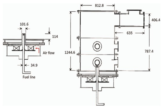
Figure 1.
NIST experimental model (dimensions in mm) [19].
In the NIST experimental model, the spray is characterized using phase Doppler interferometry (PDI). The database contains the three components of the average droplet velocity, and the density, volume, and distribution. Particle image velocimetry (PIV) was used to characterize the flow velocity near the injector, and the fluctuation in the three components of velocity (axial, radial, and tangential) as a function of their radial position at distances of 1.4, 9.5, and 17.6 mm, from the injector, and in this paper, we also consider these distances. The temperature at the outlet and on the walls, as measured by thermocouples, and the composition of the exhaust gases, are also reported.
3. Simulation Setup
3.1. Model Representation
In ANSYS Fluent, the velocity profiles are inserted as a list in the air ring inlet (Figure 2). The injector is defined as a circle with a radius of 0.28 mm. Under the discrete phase boundary condition, droplets of fuel were injected at 690 kPa after every 10 iterations of the continuum phase to match the fuel mass flow of the NIST experiments, with an equivalence ratio of 0.28 in both cases. The temperature profile for the walls of the combustion chamber was drawn from experimental data from NIST for methanol [19], whereas for hydrogen, a convection heat transfer coefficient of 20 was used, since there is natural convection around the combustion chamber. The methanol was assumed to be at ambient temperature while the hydrogen was assumed to be at 20.78 K. The outlet was defined only as it is with atmospheric pressure. As we can see from Figure 2, the NIST combustion chamber has non-centered outlet exhaust gases; however, results reported in the literature [19] have shown that the outlet position has no effect on the flow in the vicinity of the injector. This means that the simplification shown in Figure 2, could be made, where the outlet is centered. The mesh parameters were derived from a grid independence study, using the mass-weighted average temperature inside the chamber as the parameter of convergence. The mesh had a structured design with 9.2 million hexahedral elements.
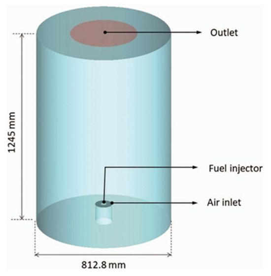
Figure 2.
Diagram of the model [1].
3.2. Turbulence Model
In cases where the density changes, as in combustion, it is necessary to make use of the Favre-averaged equations, where the Navier–Stokes equations are weighted by density, so after averaging the equations, the fluctuations in density are deleted. The Favre-averaged mass and momentum conservation equations are given in Equations (1) and (2), respectively.
In these equations, the terms and are the source terms of mass and momentum, respectively, which account for the mass (vapor) and momentum transferred between the fuel droplets and the continuous phase. is the term representing the body forces.
The SST-SAS turbulence model contains the transport equations for and ω, as show in Equations (3) and (4).
3.3. Spray Formation Model
The liquid phase was modeled using a Lagrangian approach. The spray atomization process is typically modeled using aerodynamic or wave growth theory to predict the spray parameters and droplet diameter. The pressure–swirl atomizer sub-model in Fluent, which was adapted in this study to the characteristics of the NIST experiment, is based on the “Linearized Instability Sheet Atomization” (LISA) model proposed by Schmidt [22]. The LISA model is divided into three stages: film formation, sheet breakup, and atomization, as described below.
Film formation: The centrifugal movement of the liquid inside the injector creates a cone of air surrounded by a film of liquid. The thickness of this film, t, is related to the mass flow given in Equation (5) and is the diameter of the injector outlet. u is the axial velocity at the injector outlet and depends on its internal characteristics, so it is obtained using the approximation of Han [23] given in Equation (6). is a dimensionless velocity coefficient with an estimated value of 0.7, and is a function of the injector design and pressure (see [24]). In the model, it is assumed that ∆P is known. The speed u can be obtained from Equation (7), where θ is the angle of exit of the spray.
Sheet Breakup: The model continues to assume a spectrum of wave disturbances that result in fluctuating velocities and pressures for both the liquid and gas. For waves with long wavelengths compared to the film thickness, a film decay mechanism proposed by Dombrowski and Johns [25] is adopted. If the surface disturbance has reached a value of at rupture, the breakup time τ can be calculated using Equation (8). Ω is the maximum growth rate. When the liquid film breaks, the ligaments have a length given by Equation (9), where the term is an empirical film constant with a default value of 12, as theoretically obtained by Weber [26] for liquid jets. The diameter of the ligaments formed at the breakup point can be obtained from a mass balance. If the ligaments are assumed to form from drops in the film twice per wavelength, the resulting diameter is given by Equation (10), where is the wave number corresponding to the maximum growth rate, Ω. The diameter of the ligament depends on the thickness of the film, which is a function of the breakup length and the radial distance from the centerline to the midline of the film at the atomizer outlet , see Equation (11). This mechanism is not used for short wavelengths relative to the film thickness; in this case, the ligament diameter is assumed to be linearly proportional to the wavelength that breaks the film, as described in Equation (12), where is the ligament constant and is equal to 0.5.
In both the long-wave and short-wave cases, ligament-to-droplet rupture is assumed to behave according to Weber’s capillary instability analysis [26]. This is given in Equation (13), where Oh is the Ohnesorge number, which is a combination of the Reynolds number and the Weber number.
Atomization: Once has been determined, this droplet diameter is assumed to be the most probable droplet size from a Rosin–Rammler distribution with a scattering parameter of 3.6 and a scattering angle of 10°, as suggested by Zhu [27] based on experimental data. It is important to note that the spray cone angle (60° in this case) must be specified when using this model.
3.4. Combustion Model
If the diffusivities are not assumed to be equal in combustion , meaning that the processes of species diffusion and thermal diffusion occur at different speeds, the species transport equation can be reduced to an equation for the mixture fraction as shown in Equation (14) [28], where is the source term due to mass transfer to the gas phase from fuel droplets or reactive particles. In addition, the Ansys Fluent 2021 R1 software solves a conservation equation for the variance of the mixing fraction, , based on Equation (15).
The non-premixed combustion model of fluent has a combustion sub-model called flamelets, in which the turbulent flame is assumed to consists of a set of small, stretched laminar flames. This approach is based on the idea that, if the chemical timescales are much shorter than the turbulence timescales, the fuel and oxidant will react in locally thin, one-dimensional structures normal to the stoichiometric boundary.
The properties of the laminar flamelets, such as the temperature, density, and species mass fraction as a function of the mixture fraction, are evaluated outside of the flow field calculation to produce so-called laminar flamelets libraries. This library is based on a set of relations between the scalar properties of the flow φ and the mixture fraction. To account for the effect of flame stretching due to the flow field in a real turbulent flame, the scalar dissipation rate X is incorporated as a parameter. However, in turbulent flows, the mixture fraction, and the scalar dissipation rate are statistically distributed.
The chemical–turbulence interaction model applies a statistical approach, based on probability density functions (PDFs), meanings that to evaluate the mean temperature, density, and mass fractions of the species, it is necessary to know the statistical distributions of the mixture fraction and scalar dissipation rate in the form of a joint PDF. The resulting rate of mean scalar dissipation is modeled by Equation (17), where is a constant with an assigned value of 2.0 and the variance in the lognormal distribution is equal to 2.0 [29]. The enthalpy term, H, is introduced since energy exchange is considered in the model (under the non-adiabatic condition).
4. Results and Discussion
4.1. Temperature Contour
Figure 3 shows the temperature contours for the methanol (a, b) and hydrogen (c, d) flames at different cutting planes. The first observation that can be made is the large temperature difference shown by the contours of the two fuels, both at the center of the flame and in the area surrounding the combustion chamber. For methanol, most of the volume at the center of the flame has a temperature in the range 1600–2000 C. Although there is a point of highest temperature in the PVC ring due to localized recirculation, this does not represent the general behavior of the flame. The areas surrounding the flame reach temperatures in the range 400–800 C. In the case of hydrogen, the temperatures at the center of the flame vary from 1800 to 2300 C, and this is reasonable behavior due to the high adiabatic flame temperature for this fuel. It can also be observed that there is a high recirculation zone in the area close to the fuel injector, which favors a good stoichiometric mixture where the combustion temperature reaches a maximum. The remaining areas of the chamber achieved temperatures of 800–1000 C. However, it can be seen that the SAS model produces similar maximum temperature peaks for both flames, while the LES model gives different results [1]. This means that the use of the SAS model may have a direct impact on the calculated temperatures, and further study is required to understand which measurement affects the results.
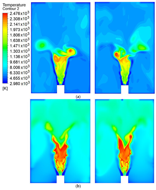
Figure 3.
Temperature contours for the (a) methanol flame and (b) hydrogen flames.
Another noteworthy aspect is the difference in lengths between the flames, as that of hydrogen is clearly greater than that of methanol, and this is an important aspect to consider when designing combustion chambers. As is characteristic of spreading flames, the centers of the flames tend to move away from the fuel injection core; that is, they do not stick to the nozzle (as in premixed combustion). This is seen for both the methanol and hydrogen flames, as the surface of the highest temperature is located above the zone of fuel atomization.
4.2. Velocity Profile
The results were validated based on experimental data from NIST [24], by comparing each component of the velocity for methanol and hydrogen. Figure 4 shows the axial, tangential, and radial velocity profiles at 9.5 mm from the injector for methanol and hydrogen. The axial velocity for hydrogen reaches a value of 5.5 m/s whereas peak velocity for methanol is approximately 10 m/s.
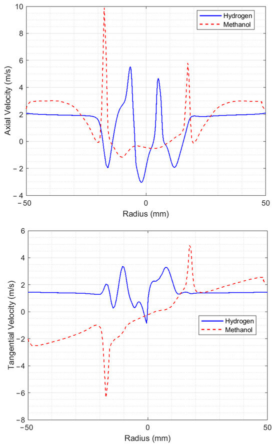

Figure 4.
Velocity profiles at 9.5 mm from the injector.
The higher speed of the air accelerated by methanol compared to hydrogen is due to the presence of a coherent structure in which the reaction occurs, meaning that the speed of the air is increased. The maximum values of the axial velocity for hydrogen are located closer to the central axis of the injector, which may be caused by the difference in densities between the fuels.
Since the hydrogen is injected with greater speed, the film of fuel leaving the injector can travel a greater distance without beginning to fracture into ligaments and, subsequently, into drops. Similar behavior is also seen for both axial speeds. From the positive speed peaks, the maximum speeds are found in the zone with negative diameter whereas the second highest speeds for the different fuels are found in the positive zone. The tangential velocities reach peak values of 3.5 m/s and 5 m/s for hydrogen and methanol, respectively. There are notable differences in the behaviors of these velocities; for methanol, a predominance of speeds is observed in the fourth quadrant of the coordinate axis, (i.e., negative speeds), while in the second quadrant, almost symmetrical but opposite speeds are obtained. The latter may be due to air recirculation in this part of the combustion chamber. For the radial velocities, it is easy to see that these are higher for hydrogen, with a maximum value of 7 m/s, and for methanol, the maximum value is 1 m/s.
Figure 5 shows the axial, tangential, and radial velocity profiles at 17.6 mm from the injector for both methanol and hydrogen. The first thing to note is the increase in speeds for methanol compared to that at 9.5 mm of the injector, as a result of the coherent structures present, where part of the combustion reaction also occurs. The axial and tangential velocity graphs show behavior that is almost proportional to that at 9.5 mm from the injector. The maximum air velocities for the hydrogen flame remain practically the same as at 9.5 mm from the injector, except for the radial velocity, which decreases considerably to a maximum value of 2.6 m/s.
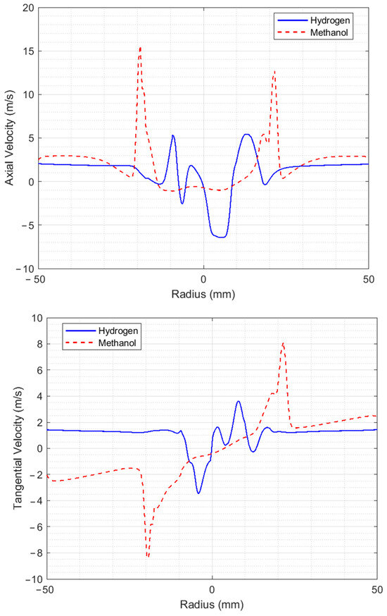
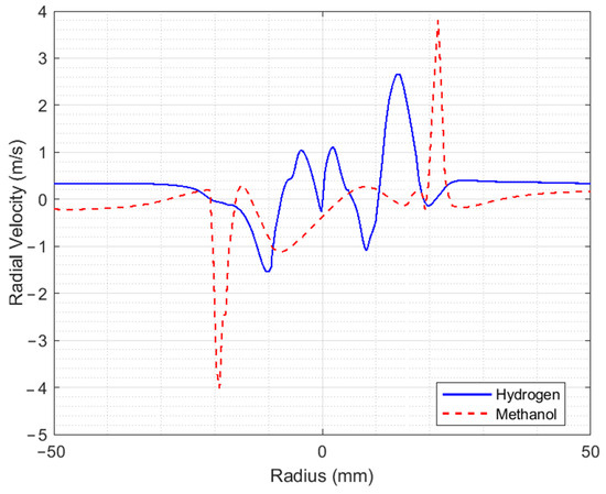
Figure 5.
Velocity profiles at a distance of 17.6 mm from the injector.
4.3. Coherent Structures
Figure 6 and Figure 7 show the coherent structures of the methanol and hydrogen flames at different values of the Q criteria. For methanol, a fully developed PVC is seen, unlike the results reported by Guevara et al. [1,21], in which only a ringed vortex was seen at the central axis of the flame. This difference may be due to the velocity profiles used at the entrance to the combustion chamber for the SAS model. The PVC of the methanol flame coils along the axial axis, and as it rotates, it creates a low-pressure zone in the east center. This low-pressure area attracts the slower low-density flow that is about to leave the combustion chamber, thus creating a recirculation structure at the exhaust gas outlet. For the methanol flame with values Q = 0.002 and Q = 0.003, a third structure similar to a PVC can be seen that moves behind the main one, and this forms part of the vortex cooling zone.
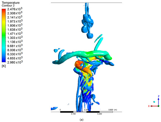
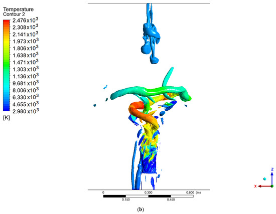
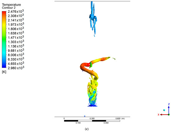
Figure 6.
Coherent structures in the methanol flame: (a) Q = 0.002, (b) Q = 0.003, (c) Q = 0.006.
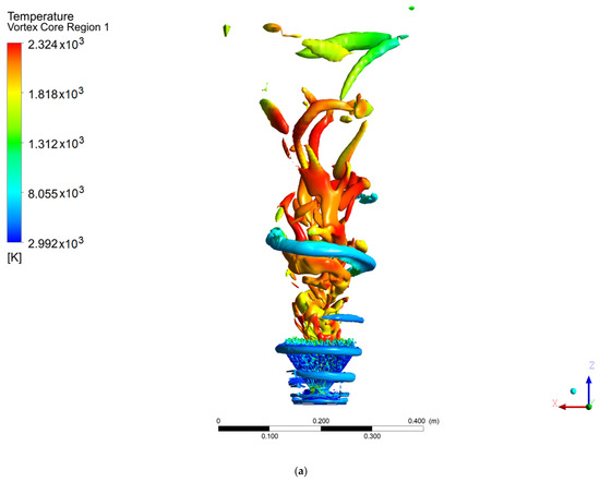
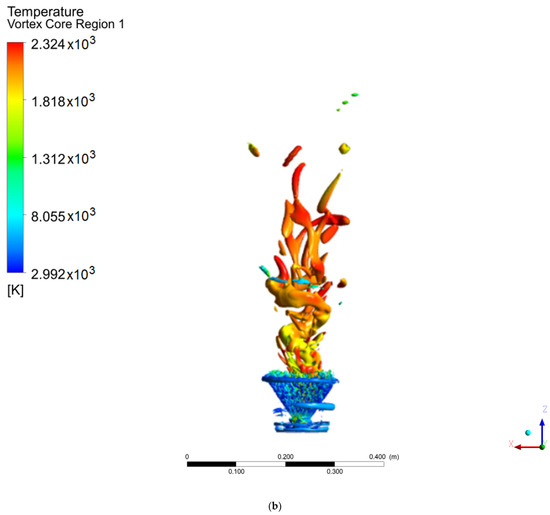
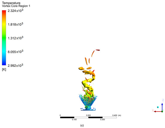
Figure 7.
Coherent structures in the hydrogen flame: (a) Q = 0.002, (b) Q = 0.003, (c) Q = 0.006.
In contrast, the hydrogen flame develops a ringed structure, as reported by Guevara [1,21], as well as the PVC centered on the axial axis. These ringed vortices around the flame arise as a consequence of the velocity gradient of the air when it enters the chamber; due to the non-slip condition at the walls of the swirler, a velocity gradient is created. This type of structure is common when a fluid is injected into a medium with a stationary fluid. The methanol flame does not show this structure, due to the width of the flame at the base of the injector, since before the rings develop, the fluid adheres to the flame. It should be noted that the PVC of the methanol flame reached a larger diameter and a greater distance or height than the hydrogen flame (this is easier to see for a value of Q = 0.006), the point from which the transition zone and a 100% turbulent flow begins.
Unlike the results from the SAS model, the work carried out by Guevara [1] using the LES model did not show a PVC-shaped structure, with ringed vortex structures being observed instead.
The following figures are presented to try to characterize the velocity field within the PVC. This visualization a more global approach than the one normally used, as information is extracted from the iso-surfaces rather than measuring the velocity components in a single line as commonly done with a laser PIV. This represents an advantage of CFD over experimental measurement methods. The PVC considered here corresponds to that seen in the SAS simulation with a Q criterion of 0.003, and the velocity components were extracted from this surface. This approach was applied to both the methanol flame (Figure 8) and the hydrogen flame (Figure 9).
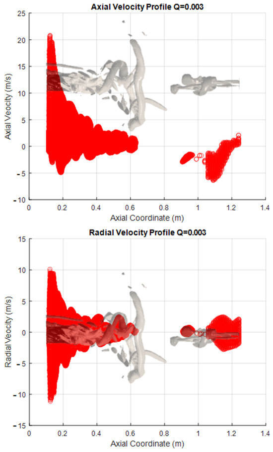
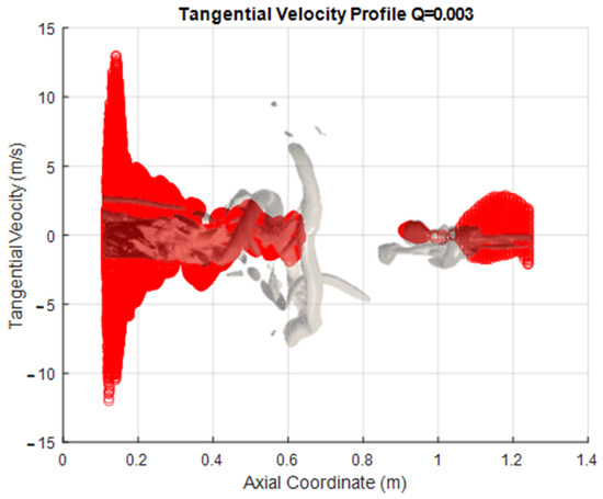
Figure 8.
Velocity Profiles of the vortex core for methanol.
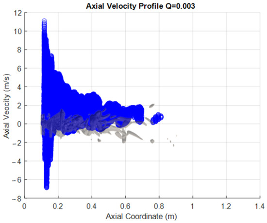
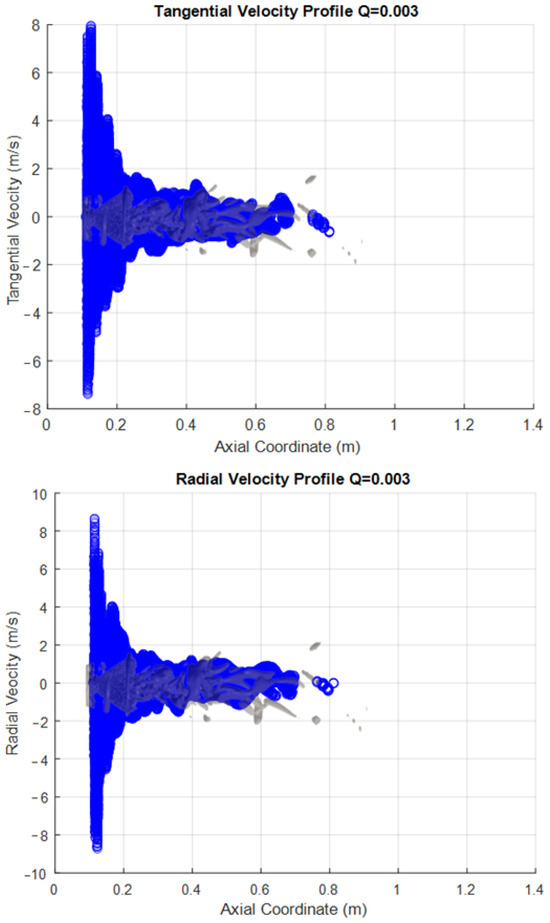
Figure 9.
Velocity Profiles of the vortex core for hydrogen.
As a 3D surface, each profile has been plotted only against the axial coordinate of the combustion chamber. The representation of the vortex is reflected in the figures. This representation lets us see the range or limits of the variable that exist within the surface; these data also include all points perpendicular (z y −z coordinate) to the sheet (the x, y plane). The vortex is described by around 50,000 points in space to which each one corresponds to a value for each extracted variable.
One interesting observation that can be made when the information is represented in this way is that both the radial and tangential components show similar behavior in the axial direction. This is as expected, since the rotary movement of the PVC has its axis at the center of the combustion chamber, and there are speed fluctuations in this area. In contrast, however, the axial component does not show this behavior. This is because there are losses of kinetic energy from the area close to the atomization (where the combustion begins) until the end of the route through the chamber, as the progressively decrease the speed.
5. Conclusions
The global temperature in the combustion chamber for hydrogen was found to be higher than that for the methanol flame.
When the SAS model was used, similar maximum temperature peaks were obtained for both flames; however, these results do not align with those of studies previously carried out with the LES model. This may imply that the SAS model in general has a direct impact on the calculated temperatures and should be studied further.
The velocity profiles of methanol and hydrogen are similar, due to the presence of the PVC. The symmetry in the tangential and axial components indicates the spinning of the flow due to the presence of a coherent structure. The reason why the peak in the tangential component for methanol is higher than for the hydrogen is due to the angle of the PVC; as it becomes more open, more tangential velocity is needed to maintain the coherent structure going on, this is fed back by the process of combustion.
Unlike the results reported by Guevara [1], the SAS model did not produce a ringed vortex near the fuel injection zone for methanol. However, it was possible to observe a well-defined PVC. This difference may be due to the different velocity profiles used at the combustion chamber inlet.
No ring vortex was seen due to the width of the methanol flame, since before the ring structure is formed, the surrounding flow of the flame adheres to it.
For the hydrogen flame, a PVC could be seen, and a ringed vortex surrounded the flame. This last type of vortex begins to join the structure of the flame because of viscosity and contributes to its cooling.
In the area where the rupture of the PVC of both flames occurs, and hence the flow is totally turbulent, stoichiometric combustion occurs with a greater proportion.
Author Contributions
Conceptualization, J.A.P.R., M.A.A.R. and O.M.H.C.; methodology, L.R.R.-L. and J.C.J.-E.; validation, M.A.A.R. and J.D.S.; analysis, J.A.P.R. and L.R.R.-L.; investigation, M.A.A.R. and O.M.H.C.; writing—original draft preparation, J.A.P.R. and M.A.A.R.; writing—review and editing, M.A.A.R. and O.M.H.C.; supervision, J.D.S. and O.M.H.C.; project administration, L.R.R.-L. and O.M.H.C.; funding acquisition, J.C.J.-E., J.D.S. and O.M.H.C. All authors have read and agreed to the published version of the manuscript.
Funding
This research was funded by the Technological Development Projects and Innovation at Instituto Politecnico Nacional (IPN), grant number SIP-20232241 and SIP-20231127.
Data Availability Statement
The data that support the findings of this study are available from the corresponding author upon reasonable request.
Conflicts of Interest
The authors declare no conflict of interest.
Nomenclature
| NIST | National Institute of Standards and Technology |
| PVC | Processing Vortex Core |
| RANS | Reynolds-averaged Navier–Stokes Equations |
| LES | Large Eddy Simulation |
| WMLES | Wall-Modeled Large-Eddy Simulation |
| ELES/ZLES | Embedded/Zonal Large Eddy Simulation |
| DNS | Direct Numerical Simulation |
| URANS | Unsteady Reynolds-averaged Navier–Stokes Equations |
| CRZ | Corner Recirculation Zone |
| CTRZ | Center Toroidal Recirculation Zone |
| PIV | Particle image velocimetry |
| CFD | Computational Fluid Dynamics |
| DES | Detached Eddy Simulation |
| DDES | Delayed Detached Eddy Simulation |
| SAS | Scale Adaptative Simulation |
| SRS | Scale-Resolving Simulation |
| SST | Shear Stress Transport |
| PISO | Pressure-Implicit with Splitting of Operators |
| Source term of mass | |
| Ω | Maximum growth rate |
| Ligament constant (equal to 0.5) | |
| Mixture fraction | |
| Source term due to mass transfer to the gas phase | |
| Source term due to body forces | |
| Variance of the mixing fraction | |
| Wave number | |
| ρ | Density |
| μ, i, j, k | Velocity component |
| , i, j, k | Average fluctuation in velocity component |
References
- Choi, S.K.; Choi, Y.S.; Jeong, Y.W.; Han, S.Y.; Van Nguyen, Q. Characteristics of Flame Stability and Gaseous Emission of Bio-Crude Oil from Coffee Ground in a Pilot-Scale Spray Burner. Energies 2020, 13, 2882. [Google Scholar] [CrossRef]
- Zhang, Y.-J.; Jamil, H.; Wei, Y.-J.; Yang, Y.-J. Displacement and Extinction of Jet Diffusion Flame Exposed to Speaker-Generated Traveling Sound Waves. Appl. Sci. 2022, 12, 12978. [Google Scholar] [CrossRef]
- Teja, K.M.V.R.; Prasad, P.I.; Reddy, K.V.K.; Banapurmath, N.R.; Soudagar, M.E.M.; Khan, T.M.Y.; Badruddin, I.A. Influence of Combustion Chamber Shapes and Nozzle Geometry on Performance, Emission, and Combustion Characteristics of CRDI Engine Powered with Biodiesel Blends. Sustainability 2021, 13, 9613. [Google Scholar] [CrossRef]
- Liang, X.; Yang, L.; Wang, G.; Li, J. Hopf Bifurcation Analysis of the Combustion Instability in a Liquid Rocket Engine. Aerospace 2022, 9, 593. [Google Scholar] [CrossRef]
- Roy, A.; Singh, S.; Nair, A.; Chaudhuri, S.; Sujith, R. Flame dynamics during intermittency and secondary bifurcation to longitudinal thermoacoustic instability in a swirl-stabilized annular combustor. Proc. Combust. Inst. 2021, 38, 6221–6230. [Google Scholar] [CrossRef]
- Drazin, P. Introduction to Hydrodynamic Stability (Cambridge Texts in Applied Mathematics); Cambridge University Press: Cambridge, UK, 2002. [Google Scholar] [CrossRef]
- Zhang, B.; Shahsavari, M.; Rao, Z.; Yang, S.; Wang, B. Contributions of hydrodynamic features of a swirling flow to thermoacoustic instabilities in a lean premixed swirl stabilized combustor. Phys. Fluids 2019, 31, 075106. [Google Scholar] [CrossRef]
- Syred, N. A review of oscillation mechanisms and the role of the precessing vortex core (PVC) in swirl combustion systems. Prog. Energy Combust. Sci. 2006, 32, 93–161. [Google Scholar] [CrossRef]
- Huang, Y.; Yang, V. Dynamics and stability of lean-premixed swirl-stabilized combustion. Prog. Energy Combust. Sci. 2009, 35, 293–364. [Google Scholar] [CrossRef]
- Spalart, P.R.; Jou, W.; Strelets, M.; Allmaras, S. Comments on the feasibility of LES for wings, and on a hybrid RANS/LES approach. In Proceedings of the First AFOSR International Conference on DNS/LES, Ruston, LA, USA, 4–8 August 1997. [Google Scholar]
- Spalart, P.R. Detached-eddy simulation. Annu. Rev. Fluid Mech. 2009, 41, 181–202. [Google Scholar] [CrossRef]
- Spalart, P.R. Strategies for turbulence modelling and simulations. Int. J. Heat Fluid Flow 2000, 21, 252–263. [Google Scholar] [CrossRef]
- Menter, F.; Kuntz, M.; Bender, R. A Scale-Adaptive Simulation Model for Turbulent Flow Predictions. In Proceedings of the 41st Aerospace Sciences Meeting and Exhibit, Reno, Nevada, 6–9 January 2003. [Google Scholar] [CrossRef]
- Egorov, Y.; Menter, F. Development and Application of SST-SAS Turbulence Model in the DESIDER Project. In Advances in Hybrid RANS-LES Modelling; Springer: Berlin/Heidelberg, Germany, 2008. [Google Scholar]
- Menter, F.; Egorov, Y. A Scale Adaptive Simulation Model using Two-Equation Models. In Proceedings of the 43rd AIAA Aerospace Sciences Meeting and Exhibit, Reno, Nevada, 10–13 January 2005. [Google Scholar]
- Zhao, R.; Xu, J.-L.; Yan, C.; Yu, J. Scale-adaptive simulation of flow past wavy cylinders at a subcritical Reynolds number. Acta Mech. Sin. 2011, 27, 660–667. [Google Scholar] [CrossRef]
- Menter, F.R.; Schütze, J.; Gritskevich, M. Global vs. Zonal Approaches in Hybrid RANS-LES Turbulence Modelling. In Progress in Hybrid RANS-LES Modelling; Springer: Berlin/Heidelberg, Germany, 2012; pp. 15–28. [Google Scholar] [CrossRef]
- Widmann, J.F.; Charagundla, S.R.; Presser, C. Aerodynamic study of a vane-cascade swirl generator. Chem. Eng. Sci. 2000, 55, 5311–5320. [Google Scholar] [CrossRef]
- Widmann, J.F.; Presser, C. A Benchmark Experimental Database for Multiphase Combustion Model Input and Validation. Combust. Flame 2002, 129, 47–86. [Google Scholar] [CrossRef]
- Guevara-Morales, G.; Huerta-Chavez, O.M.; Castorena, I.; Bernal-Orozco, R.; Cruz-Cruz, J.; Torres-Cedillo, S.G.; Abad-Romero, M. Computational Modeling of Turbulent Spray Combustion Process Using RANS and Large-Eddy Simulations. J. Aerosp. Eng. 2022, 35, 05021002. [Google Scholar] [CrossRef]
- Guevara-Morales, G.; Huerta-Chávez, O.; Arias-Montaño, A. Modelado computacional Reynolds-Averaged Navier-Stokes flamelets para el estudio del proceso de combusti’on turbulenta de sprays. Rev. Mex. Fís. 2020, 66, 56–68. [Google Scholar] [CrossRef]
- Schmidt, D.; Nouar, I.; Senecal, P.; Rutland, C.; Martin, J.; Reitz, R. Pressure-swirl atomization in the near field. SAE Trans. 1999, 108, 471–484. [Google Scholar]
- Han, Z.; Parrish, S.E.; Farrell, P.V.; Reitz, R.D. Modeling atomization processes of pressure-swirl hollow-cone fuel sprays. At. Sprays 1997, 7, 663–684. [Google Scholar] [CrossRef]
- Lefebvre, A.H. Atomization and Sprays; Hemisphere Publishing Corporation: New York, NY, USA, 1989. [Google Scholar]
- Dombrowski, N.; Johns, W. The aerodynamic instability and disintegration of viscous in sprays. Chem. Eng. Sci. 1963, 18, 203. [Google Scholar] [CrossRef]
- Weber, C. Zum Zerfall eines Flüssigkeitsstrahles. ZAMM 1931, 11, 136–154. [Google Scholar] [CrossRef]
- Zhu, S.; Roekaerts, D.; Pozarlik, A.; van der Meer, T. Eulerian–Lagrangian RANS Model Simulations of the NIST Turbulent Methanol Spray Flame. Combust. Sci. Technol. 2015, 187, 1110–1138. [Google Scholar] [CrossRef]
- ANSYS Fluent 12.0 Theory Guide; ANSYS Inc.: Canonsburg, PA, USA, 2009.
- Peters, N. Laminar diffusion flamelet models in non-premixed turbulent combustion. Prog. Energy Combust. Sci. 1984, 10, 319–339. [Google Scholar] [CrossRef]
Disclaimer/Publisher’s Note: The statements, opinions and data contained in all publications are solely those of the individual author(s) and contributor(s) and not of MDPI and/or the editor(s). MDPI and/or the editor(s) disclaim responsibility for any injury to people or property resulting from any ideas, methods, instructions or products referred to in the content. |
© 2023 by the authors. Licensee MDPI, Basel, Switzerland. This article is an open access article distributed under the terms and conditions of the Creative Commons Attribution (CC BY) license (https://creativecommons.org/licenses/by/4.0/).