

Differentiator-Based Output Feedback MPPT Controller for DFIG Wind Energy Conversion Systems with Minimal System Information


Abstract
:1. Introduction
- The proposed controller demands significantly less information about the system’s dynamic equation. The control formulation relies solely on the relative degrees between inputs and outputs, the directions of control inputs, and the measured output values.
- Owing to the absence of universal approximators, the structures of the control laws are comparatively straightforward, while still ensuring the asymptotic stability of the outputs.
- The proposed output feedback control algorithm offers a cohesive and systematic approach for crafting control laws.
- The quantity of design constants is minimal in comparison to that of other methods.
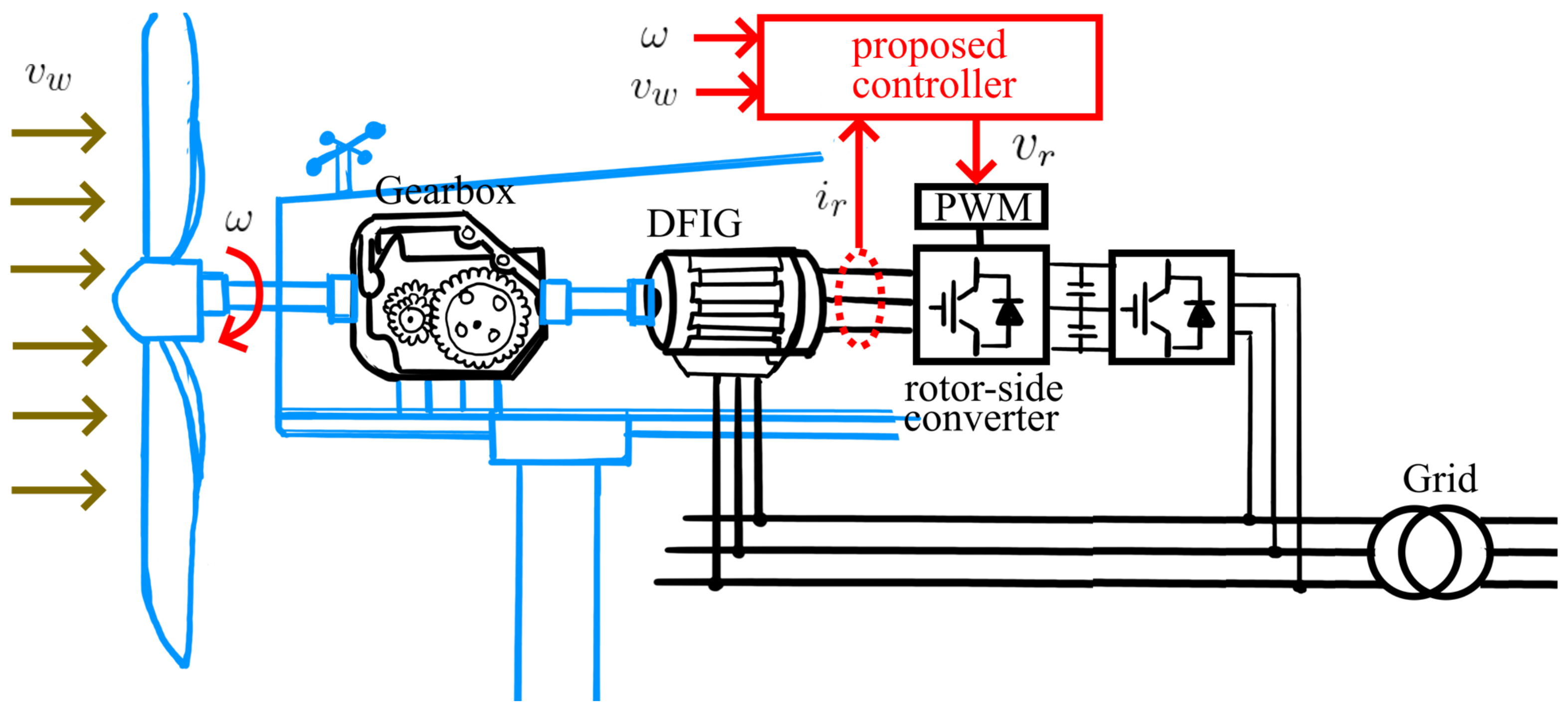
2. Dynamic Model of the WECS with DFIG
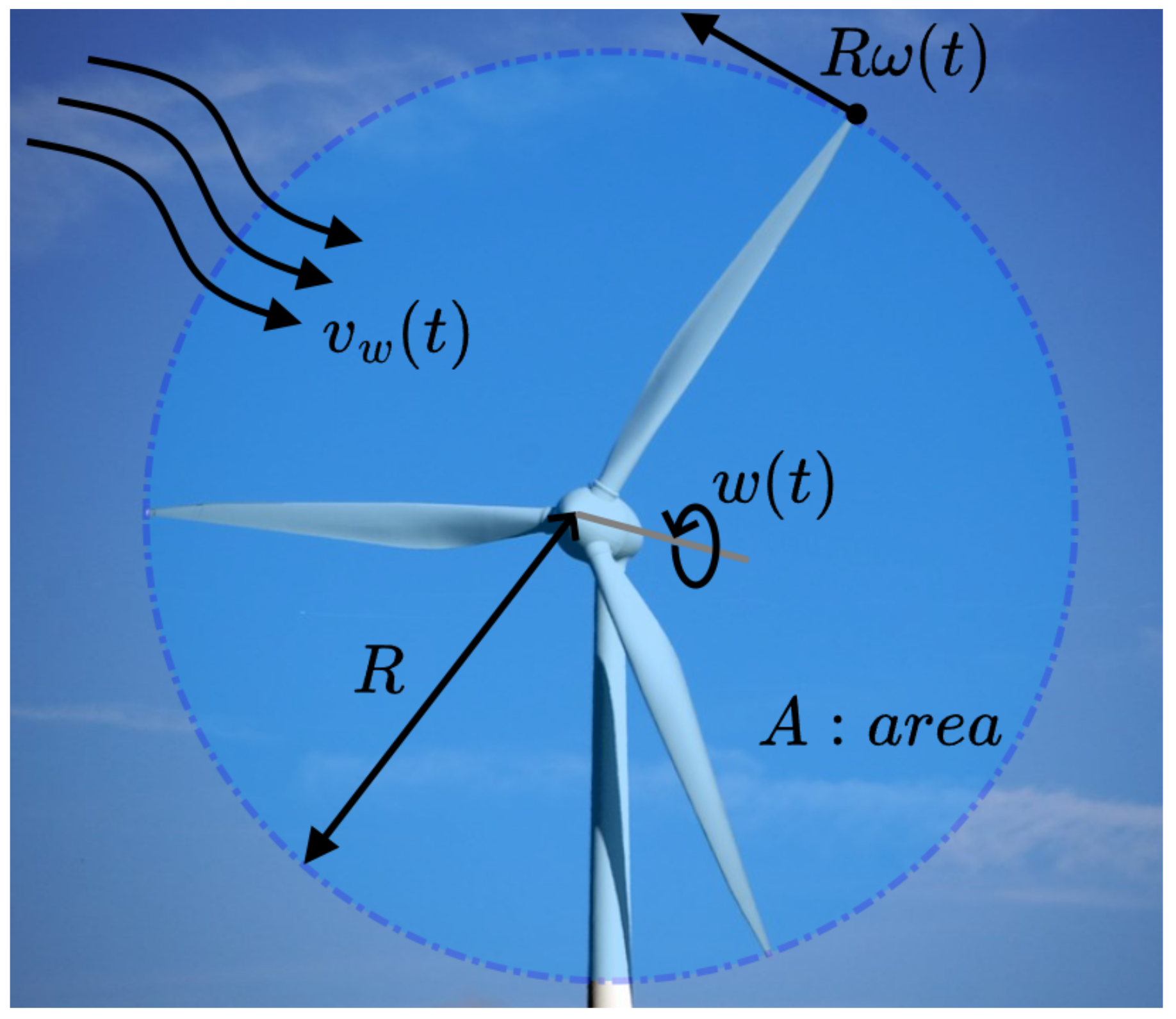
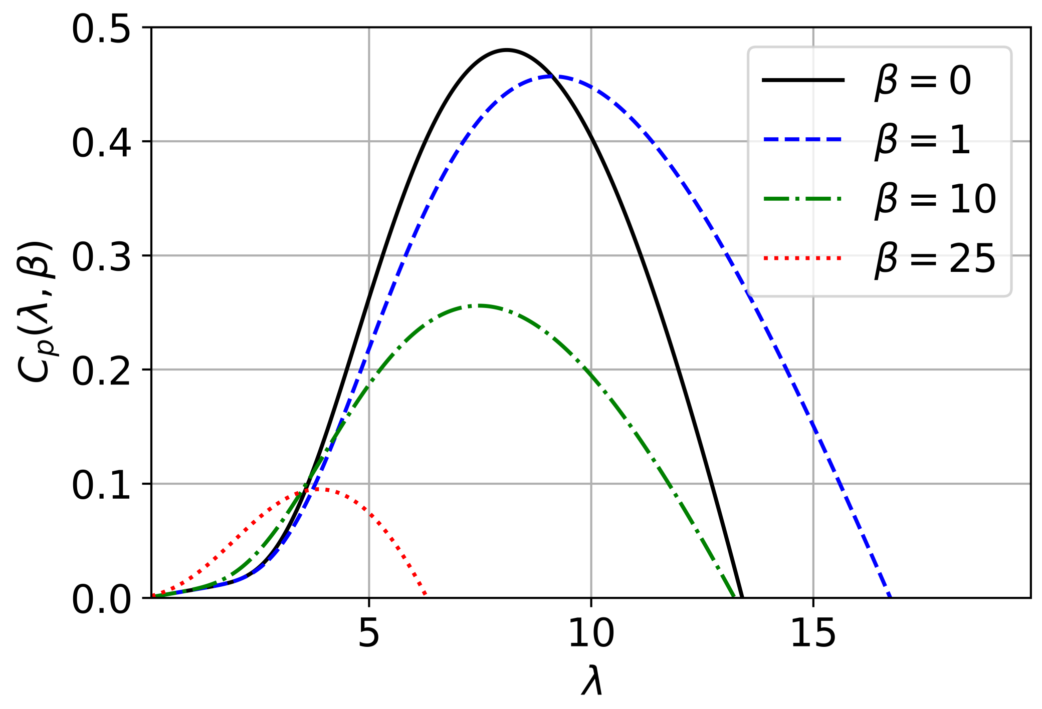
2.1. Model of WECS
2.2. Mathematical Model of DFIG
3. Design of Output Feedback Controllers
3.1. MPPT Control
3.2. Regulating to Zero
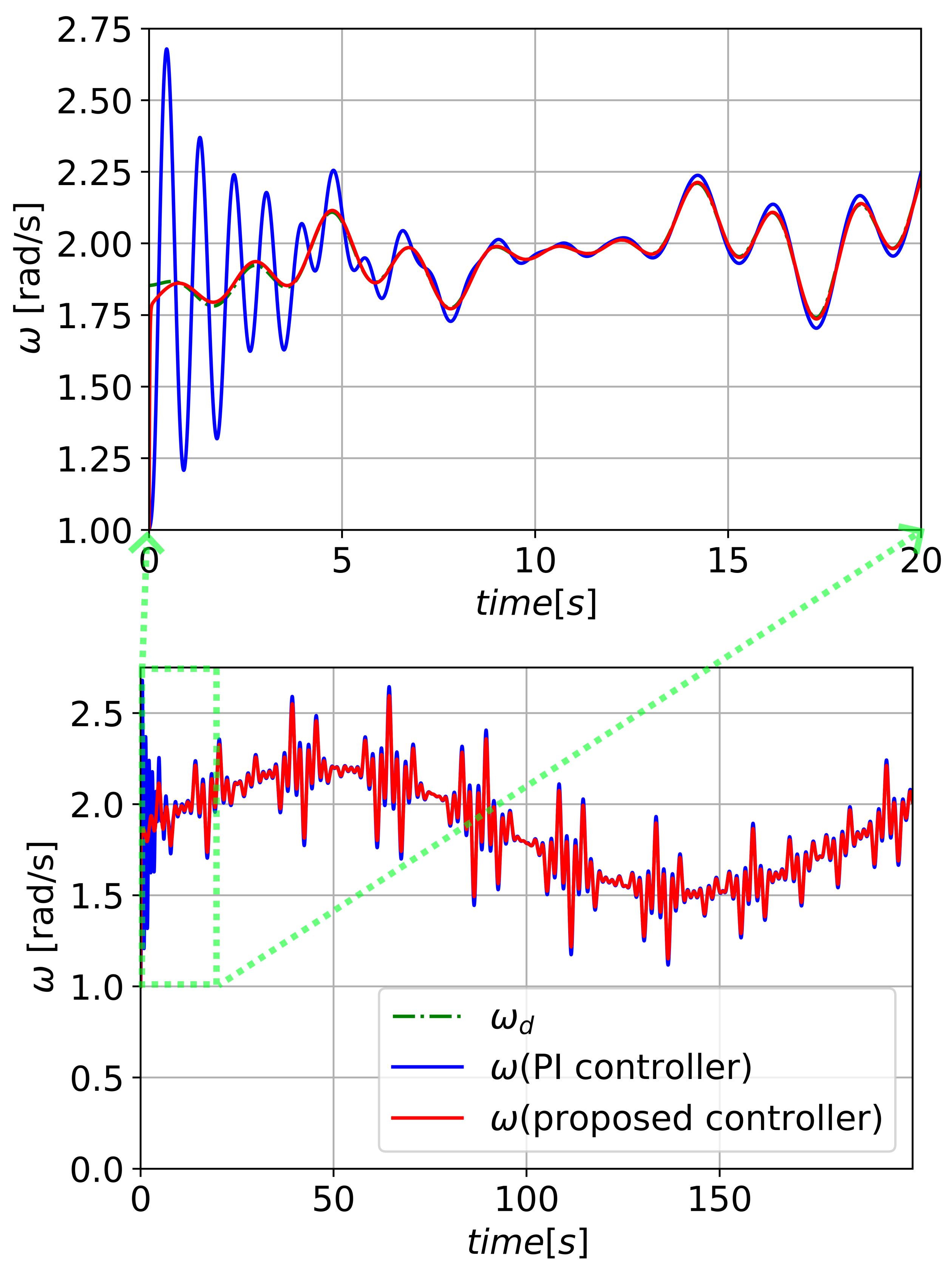
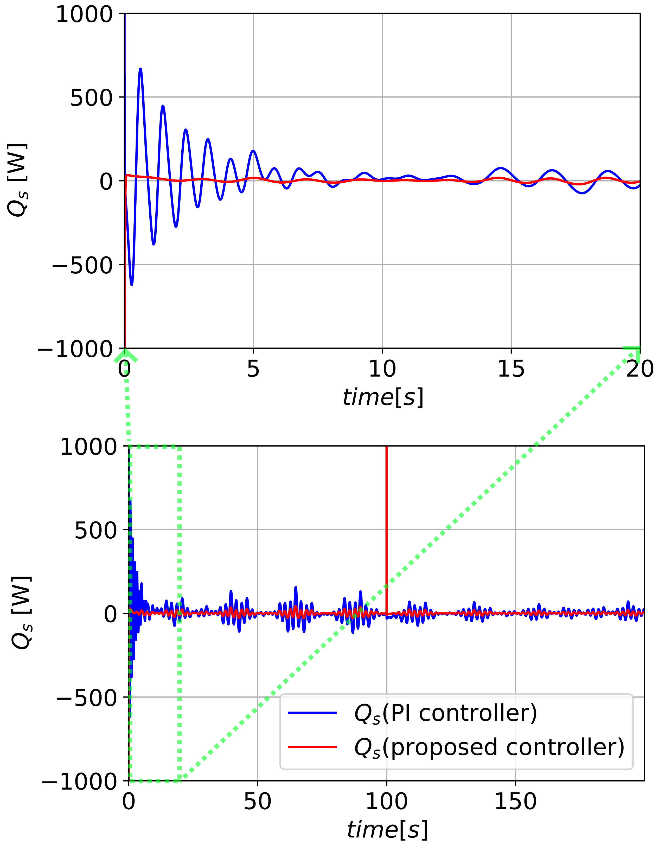
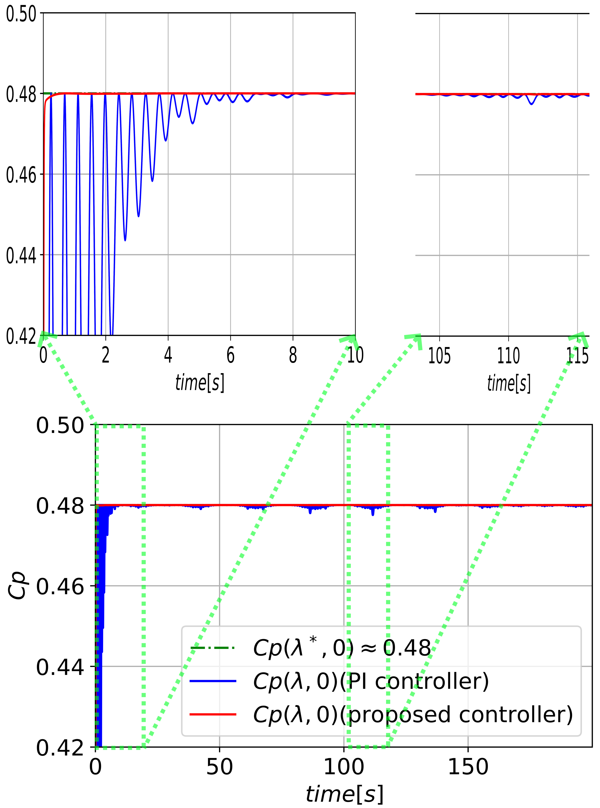
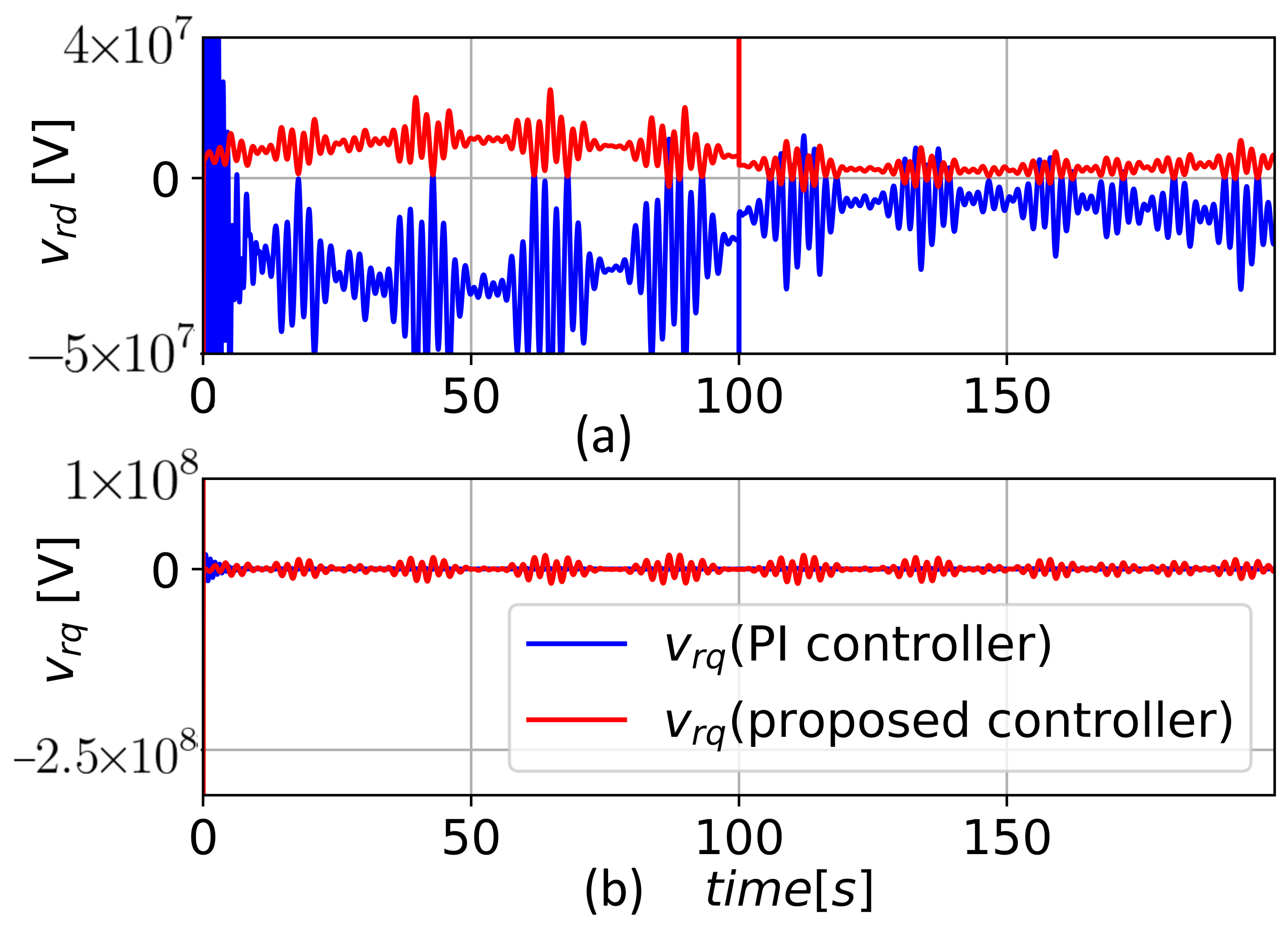
4. Simulations
5. Conclusions
Funding
Data Availability Statement
Conflicts of Interest
References
- Cardenas, R.; Pena, R.; Alepuz, S. Overview of control systems for the operation of DFIGs in wind energy applications. IEEE Trans. Ind. Electron. 2013, 60, 2776–2798. [Google Scholar] [CrossRef]
- Jadhav, H.T.; Roy, R. A comprehensive review on the grid integration of doubly fed induction generator. Int. J. Electr. Power Energy Syst. 2013, 49, 8–18. [Google Scholar] [CrossRef]
- El-Naggar, M.F.; Mosaad, M.I.; Hasanien, H.M.; AbdulFattah, T.A.; Bendary, A.F. Elephant herding algorithm-based optimal PI controller for LVRT enhancement of wind energy conversion systems. Ain Shams Eng. J. 2021, 12, 599–608. [Google Scholar] [CrossRef]
- Mossad, M.I.; Sabiha, N.A.; Abu-Siada, A.; Taha, I.B.M. Application of Superconductors to Suppress Ferroresonance Overvoltage in DFIG-WECS. IEEE Trans. Energy Convers. 2021, 37, 766–777. [Google Scholar] [CrossRef]
- Hamane, B.; Doumbia, M.L.; Bouhamida, M.; Draou, A.; Chaoui, H.; Benghanem, M. Comparative study of PI, RST, sliding mode and fuzzy supervisory controllers for DFIG based wind energy conversion system. Int. J. Renew. Energy Res. 2015, 5, 1174–1185. [Google Scholar]
- Levant, A. Higher-order sliding modes, differentiation and output-feedback control. Int. J. Control 2003, 76, 924–941. [Google Scholar] [CrossRef]
- Levant, A.; Livne, M. Weighted Homogeneity and Robustness of Sliding Mode Control. Automatica 2016, 72, 186–193. [Google Scholar] [CrossRef]
- Tong, S.; Liu, C.; Li, Y. Fuzzy-adaptive decentralized output-feedback control for large-scale nonlinear systems with dynamical uncertainties. IEEE Trans. Fuzzy Syst. 2010, 18, 845–861. [Google Scholar] [CrossRef]
- Tong, S.C.; Li, Y.M.; Zhuang, H.-G. Adaptive neural network decentralized backstepping output-feedback control of nonlinear large-scale systems with time-delays. IEEE Trans. Neural Netw. 2011, 22, 1073–1086. [Google Scholar] [CrossRef]
- Li, J.; Chen, W.; Li, J.-M. Adaptive NN output-feedback decentralized stabilization for a class of large-scale stochastic nonlinear strict-feedback systems. Int. J. Robust Nonlinear Control 2011, 21, 452–472. [Google Scholar] [CrossRef]
- Tong, S.; Li, Y.; Liu, Y. Adaptive fuzzy output feedback decentralized control of pure-feedback nonlinear large-scale systems. Int. J. Robust Nonlinear Control 2014, 24, 930–954. [Google Scholar] [CrossRef]
- Yang, Y.; Yue, D.; Xue, Y. Decentralized adaptive neural output feedback control of a class of large-scale time-delay systems with input saturation. J. Frankl. Inst. 2015, 352, 2129–2151. [Google Scholar] [CrossRef]
- Jiang, X.; Mu, X.; Hu, Z. Decentralized Adaptive Fuzzy Tracking Control for a Class of Nonlinear Uncertain Interconnected Systems with Multiple Faults and DoS Attack. IEEE Trans. Fuzzy Syst. 2020, 29, 3130–3141. [Google Scholar] [CrossRef]
- Wang, H.; Xiaoping, P.; Bao, J.; Xie, X.-J.; Li, S. Adaptive Neural Output-Feedback Decentralized Control for Large-Scale Nonlinear Systems with Stochastic Disturbances. IEEE Trans. Neural Netw. Learn. Syst. 2020, 31, 972–983. [Google Scholar] [CrossRef] [PubMed]
- Ma, Z.; Ma, H. Decentralized Adaptive NN Output-Feedback Fault Compensation Control of Nonlinear Switched Large-Scale Systems with Actuator Dead-Zones. IEEE Trans. Syst. Man Cybern. Syst. 2020, 50, 3435–3447. [Google Scholar] [CrossRef]
- Wang, H.; Chen, B.; Lin, C.; Sun, Y. Neural-network-based decentralized output-feedback control for nonlinear large-scale delayed systems with unknown dead-zones and virtual control coefficients. Neurocomputing 2020, 424, 255–267. [Google Scholar] [CrossRef]
- Bechlioulis, C.P.; Rovithakis, G.A. A low-complexity global approximation-free control scheme with prescribed performance for unknown pure feedback systems. Automatica 2014, 50, 1217–1226. [Google Scholar] [CrossRef]
- Zhang, J.-X.; Yang, G.-H. Low-Complexity Tracking Control of Strict-Feedback Systems with Unknown Control Directions. IEEE Trans. Autom. Control 2019, 64, 5175–5182. [Google Scholar] [CrossRef]
- Zhang, J.-X.; Yang, G.-H.; Ding, W. Global Output-Feedback Prescribed Performance Control of Nonlinear Systems with Unknown Virtual Control Coefficients. IEEE Trans. Autom. Control 2022, 67, 6904–6911. [Google Scholar] [CrossRef]
- Guo, Z.; Oliveira, T.R.; Guo, J.; Wang, Z. Performance-Guaranteed Adaptive Asymptotic Tracking for Nonlinear Systems with Unknown Sign-Switching Control Direction. IEEE Trans. Autom. Control 2023, 68, 1077–1084. [Google Scholar] [CrossRef]
- Park, J.-H.; Kim, S.-H.; Park, T.-S. Approximation-Free Output-Feedback Non-Backstepping Controller for Uncertain SISO Nonautonomous Nonlinear Pure-Feedback Systems. Mathematics 2019, 7, 456. [Google Scholar] [CrossRef]
- Park, J.-H.; Kim, S.-H.; Lee, D.-H. Decentralized Output-Feedback Controller for Uncertain Large-Scale Nonlinear Systems Using Higher-Order Switching Differentiator. IEEE Access 2021, 9, 21227–21235. [Google Scholar] [CrossRef]
- Wang, J.; Bo, D.; Miao, Q.; Li, Z.; Wu, X.; Lv, D. Maximum power point tracking control for a doubly fed induction generator wind energy conversion system based on multivariable adaptive super-twisting approach. Int. J. Electr. Power Energy Syst. 2021, 124, 106347. [Google Scholar] [CrossRef]
- Xiong, L.; Li, P.; Wu, F.; Ma, M.; Khan, M.W.; Wang, J. A coordinated high-order sliding mode control of DFIG wind turbine for power optimization and grid synchronization. Int. J. Electr. Power Energy Syst. 2019, 105, 679–689. [Google Scholar] [CrossRef]
- Shihabudheen, K.V.; Raju, S.K.; Pillai, G.N. Control for grid-connected DFIGbased wind energy system using adaptive neuro-fuzzy technique. Int. Trans. Electr. Energy Syst. 2018, 28, e2526. [Google Scholar] [CrossRef]
- Kumar, R.; Agrawal, H.P.; Shah, A.; Bansal, H.O. Maximum power point tracking in wind energy conversion system using radial basis function based neural network control strategy. Sustain. Energy Technol. Assess. 2019, 36, 100533. [Google Scholar] [CrossRef]
- Aissaoui, H.E.; Ougli, A.E.; Tidhaf, B. Neural Networks and Fuzzy Logic Based Maximum Power Point Tracking Control for Wind Energy Conversion System. Adv. Sci. Technol. Eng. Syst. J. 2021, 6, 586–592. [Google Scholar] [CrossRef]
- Sami, I.; Ullah, S.; Amin, S.U.; Al-Durra, A.; Ullah, N.; Ro, J.S. Convergence Enhancement of Super-Twisting Sliding Mode Control Using Artificial Neural Network for DFIG-Based Wind Energy Conversion Systems. IEEE Access 2022, 10, 97625–97641. [Google Scholar] [CrossRef]
- Yan, S.; Gu, Z.; Park, J.H.; Xie, X. Adaptive Memory-Event-Triggered Static Output Control of T–S Fuzzy Wind Turbine Systems. IEEE Trans. Fuzzy Syst. 2022, 30, 3894–3904. [Google Scholar] [CrossRef]
- Yan, S.; Gu, Z.; Park, J.H.; Xie, X. Sampled Memory-Event-Triggered Fuzzy Load Frequency Control for Wind Power Systems Subject to Outliers and Transmission Delays. IEEE Trans. Cybern. 2023, 53, 4043–4053. [Google Scholar] [CrossRef]
- Jing, F.; Liu, W.; Sun, H.; Yu, F.; Wang, K. Prescribed performance finite-time control of wind energy conversion systems with input constraint and system uncertainty. Int. Trans. Electr. Energy Syst. 2021, 32, e13215. [Google Scholar] [CrossRef]
- Lv, G.; Cong, S.; Liu, Y.; Peng, Z.; Wang, D. Maximum Power Tracking Control of Wind Energy Conversion Systems Based on Prescribed Performance Function and Extended State Observer. In Proceedings of the 2018 3rd International Conference on Advanced Robotics and Mechatronics (ICARM), Singapore, 18–20 July 2018; pp. 829–834. [Google Scholar] [CrossRef]
- Park, J.-H.; Kim, S.-H.; Park, T.-S. Asymptotically Convergent Higher-Order Switching Differentiator. Mathematics 2020, 8, 185. [Google Scholar] [CrossRef]
- Boukhezzar, B.; Siguerdidjane, H. Nonlinear control with wind estimation of a DFIG variable speed wind turbine for power capture optimization. Energy Convers. Manag. 2009, 50, 885–892. [Google Scholar] [CrossRef]
- Park, J.-H.; Kim, S.-H.; Park, T.-S. Differentiator-Based Output-Feedback Controller for Uncertain Nonautonomous Nonlinear Systems with Unknown Relative Degree. IEEE Access 2020, 8, 172593–172600. [Google Scholar] [CrossRef]
- Park, J.-H.; Kim, S.-H.; Park, T.-S. Asymptotically convergent switching differentiator. Int. J. Adapt. Control Signal Process. 2019, 33, 557–566. [Google Scholar] [CrossRef]
- Hou, Z.; Chi, R.; Gao, H. An Overview of Dynamic-Linearization-Based Data-Driven Control and Applications. IEEE Trans. Ind. Electron. 2017, 64, 4076–4090. [Google Scholar] [CrossRef]
- Hunter, J.D. Matplotlib: A 2D graphics environment. Comput. Sci. Eng. 2007, 9, 90–95. [Google Scholar] [CrossRef]


| Notation | Description |
|---|---|
| wind speed | |
| inertia of the turbine | |
| inertia of the generator | |
| gear ratio | |
| J | total inertia (=) |
| D | damping constant of the wind turbine |
| air density | |
| R | radius of the blade |
| A | the area swept by the blades |
| rotational velocity of the wind turbine’s rotor | |
| tip-speed ratio (=) | |
| optimal value of tip-speed ratio | |
| blade pitch angle | |
| power coefficient function defined as (3) | |
| system constants in the function | |
| stator electrical angular speed | |
| stator resistance | |
| rotor resistance | |
| stator inductance | |
| rotor inductance | |
| mutual inductance | |
| number of pole pairs | |
| , | d- and q-axis currents of the generator’s rotor |
| , | d- and q-axis voltages of the generator’s rotor |
| d-axis flux of the generator’s stator | |
| , | active and reactive powers |
| Notation | Value | Description |
|---|---|---|
| 0.5176 | constant in (3) | |
| 116 | constant in (3) | |
| 0.4 | constant in (3) | |
| 5 | constant in (3) | |
| 21 | constant in (3) | |
| 0.0068 | constant in (3) | |
| stator electrical angular speed | ||
| 0.005 | stator resistance | |
| 0.228 | rotor resistance | |
| 0.407 | stator inductance | |
| 0.299 | rotor inductance | |
| 0.0016 | mutual inductance | |
| 4 | number of pole pairs | |
| J | total inertia | |
| D | 400 | damping constant |
| 1.08 | air density | |
| R | 35 | radius of the blade |
| 43.165 | gear ratio | |
| 8.1072 | optimal value of |
Disclaimer/Publisher’s Note: The statements, opinions and data contained in all publications are solely those of the individual author(s) and contributor(s) and not of MDPI and/or the editor(s). MDPI and/or the editor(s) disclaim responsibility for any injury to people or property resulting from any ideas, methods, instructions or products referred to in the content. |
© 2023 by the author. Licensee MDPI, Basel, Switzerland. This article is an open access article distributed under the terms and conditions of the Creative Commons Attribution (CC BY) license (https://creativecommons.org/licenses/by/4.0/).
Share and Cite
Park, J.-H. Differentiator-Based Output Feedback MPPT Controller for DFIG Wind Energy Conversion Systems with Minimal System Information. Energies 2023, 16, 7068. https://doi.org/10.3390/en16207068
Park J-H. Differentiator-Based Output Feedback MPPT Controller for DFIG Wind Energy Conversion Systems with Minimal System Information. Energies. 2023; 16(20):7068. https://doi.org/10.3390/en16207068
Chicago/Turabian StylePark, Jang-Hyun. 2023. "Differentiator-Based Output Feedback MPPT Controller for DFIG Wind Energy Conversion Systems with Minimal System Information" Energies 16, no. 20: 7068. https://doi.org/10.3390/en16207068
APA StylePark, J.-H. (2023). Differentiator-Based Output Feedback MPPT Controller for DFIG Wind Energy Conversion Systems with Minimal System Information. Energies, 16(20), 7068. https://doi.org/10.3390/en16207068