Modeling and Simulating Wind Energy Generation Systems by Means of Co-Simulation Techniques

Abstract

This paper presents the development of a wind energy conversion system co-simulation based on the Functional Mock-up Interface standard aiming at contributing to the development of co-simulation of large electrical power systems by means of open-source and standardized computational tools. Co-simulation enables the computational burden of a monolithic simulation to be shared among several processing units, significantly reducing processing time. Through the Functional Mock-up Interface standard, developed models are encapsulated into Functional Mock-up Unit, providing an extra means for the protection of intellectual property, a very appealing feature for end users, both in industry and academia. To achieve the decoupling of the subsystems, the Bergeron ideal transmission line model will be used, with travel time equal to the simulation time-step. The computational performance and effectiveness of the proposed co-simulation technique was evaluated with a wind power plant with 50 wind turbines. The system digital models were developed into Modelica language, while co-simulation was implemented in Python.

1. Introduction

Transient stability (TS) and Electromagnetic transients (EMT) programs are widely used simulation tools in a variety of studies in power systems [1]. TS simulation, also known as electromechanical dynamic simulations, is fast because the associated modeling is based on the positive-sequence phasor domain, which renders them suitable for handling large-scale networks [2]. On the other hand, EMT simulation handles highly detailed network models, which causes them to be much more computationally expensive. Consequently, the last one is often used to simulate only small portions of the network [3].

This limitation has driven the search for alternatives capable of performing EMT simulations in large-scale systems. An alternative relies on frequency-dependent network equivalents to represent regions that are not of interest in the study. To be accurate, such equivalents need to include the frequency response of positive and zero sequence networks. Computing a frequency scan, however, is usually a laborious task. Furthermore, a passivity characteristic needs to be ensured for the synthesized equivalent model so that the time simulation is stable, which is not always possible [4,5].

Another alternative is to partition the system into smaller subsystems so that the computational effort can be shared among several processing units. Using co-simulation techniques, complex and interconnected systems, such as electrical power systems, can be partitioned into smaller subsystems, where each subsystem can be modeled and simulated on its own [6,7]. Furthermore, such partitioning allows one to use distinct modeling alternatives and solution algorithms, which may be more appropriate or more efficient to each one of the subsystems [8].

In this context, commercial offline EMT simulation tools as well as those applied to real-time simulation, such as PSCAD/EMTDC, EMTP, RSCAD, and HYPERSIM, for instance, employ partitioning techniques in order to increase the computational performance of the simulations. In these tools, subsystems are decoupled at their boundaries by means of transmission lines that introduce a natural time delay intrinsic to its model [9].

This approach allows using a fictitious Bergeron transmission line model [3], with a propagation time identical to the simulation time-step, to couple two electrical subsystems or regions where a real transmission line does not necessarily exist. The dynamic behavior introduced by the Bergeron transmission line model at the point of connection of adjacent subsystems does not affect the accuracy or numerical stability of the simulation.

Tremblay et al. [10] provide the basic steps to create the virtual transmission line model to couple subsystems in a co-simulation. The line characteristic impedance $Z_c$ is used as the internal impedance connected to the input and output terminals of the Bergeron model. In three-phase applications, the line-coupled equations, in the phase domain, are commonly decoupled in the modal domain [3]. Subsequently, if the line is ideally transposed, the modes are fully decoupled and a single-phase Bergeron line represents each propagation mode.

In [11], the authors use a part of an existing transmission line in the original network as a decoupling element between two subsystems. In this case, the characteristic impedance value must equal that of the existing line, while the delay between the input and output terminals will depend on the equivalent length of the decoupling line. Although this approach does not impose any restrictions on the signals exchanged between the two subsystems, the authors report three limitations. (i) The method cannot be used when the line length is short and the propagation delay is smaller than the EMT time-step; (ii) in real-time couplings, due to the adoption of a non-iterative solution between TS-EMT, it was necessary to reduce the TS time-step, especially during major disturbances in the power system; (iii) the lines used in the interface should ideally be transposed.

Another approach would be to choose the virtual line characteristic impedance $Z_c$ without any correlation with an actual line. As an example, it can be adjusted to minimize any unwanted behavior, such as a reflected wave at the virtual line terminals [12].

Motivation and Contribution of the Work

Therefore, this work proposes the use of the fictitious Bergeron model to perform the decoupling of the co-simulated subsystems, where the latency of the model equals the time-step used in the simulation. The main contributions can be summarized as follows:

(i)

Mathematical Models: The compilation of a set of models for Wind Energy Conversion System (WECS) units, allowing for a comprehensive representation of the system’s dynamic behavior for the industrial frequency range. Furthermore, these models serve as valuable tools for analyzing and optimizing the performance of the interconnected components in various operating conditions.

(ii)

Interface Standard: The co-simulation is attained with the aid of the Functional Mock-up Interface (FMI) standard [13], which aims at making models, developed for different simulation tools, compatible. As one possibility for subsystem integration, the FMI standard allows one to encapsulate whole subsystems into a single Functional Mock-up Unit (FMU), which contains a machine-compiled mathematical description of the subsystem at hand. Depending on the FMU type, a numerical solver can also be embedded in it. As a by-product of the FMU encapsulation, provided by the FMI standard, one can identify the improved intellectual property protection, which can be vital for certain applications.

(iii)

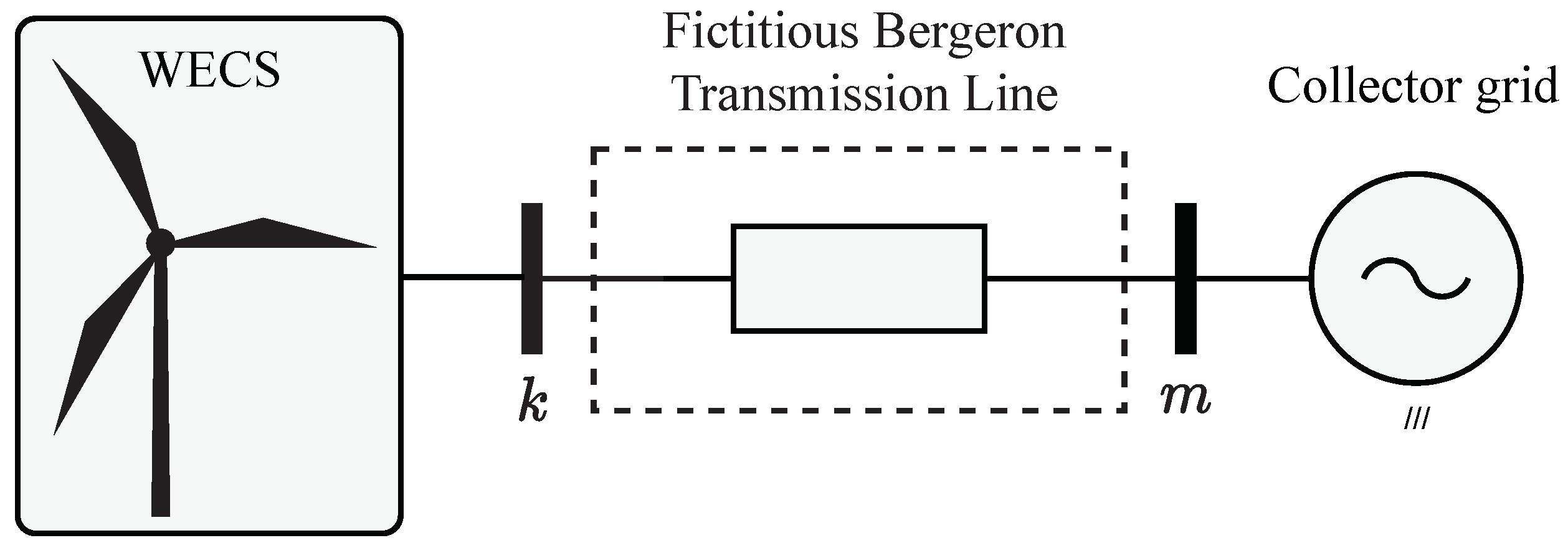
Digital Simulation: The implementation of a parallel-processed co-simulation framework based on open-source tools and standards for inter-process communication and mathematical model interfaces is detailed. The use of a fictitious Bergeron transmission line model, which partitions large-scale power systems into smaller subsystems, provided accurate and stable results, by means of co-simulation techniques.

(iv)

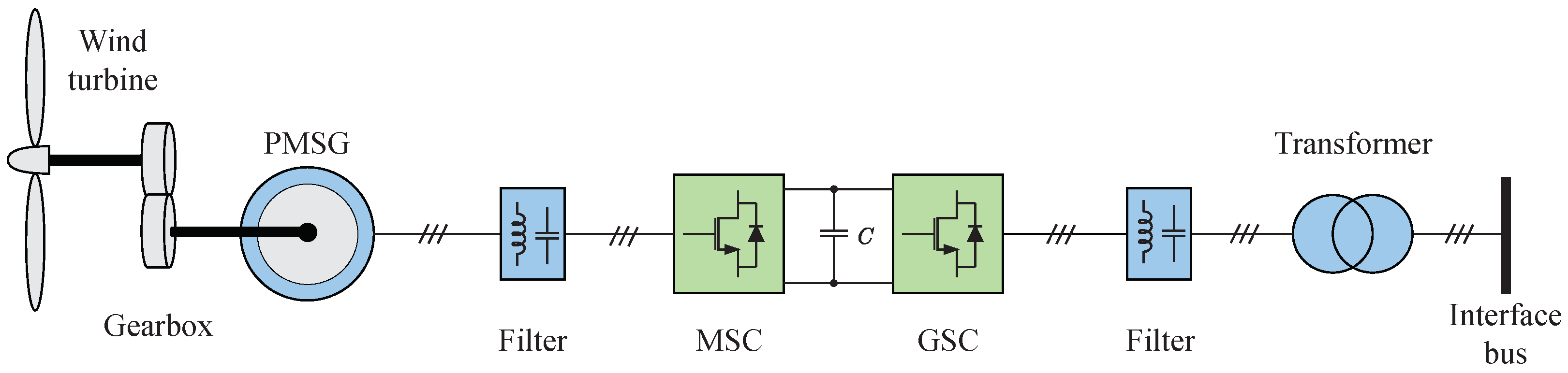
Evaluation and Testing: To validate the proposed approach, simulations considering a wind power plant (WPP) with an AC medium-voltage collector system with 50 wind generation units are performed. The WECS adopted in this paper is constituted by a wind turbine coupled to a permanent magnet synchronous generator through a gearbox and back-to-back two-level voltage-source-based power converters. The mathematical models are developed into Modelica language [14], whereas the co-simulation master algorithm is implemented in Python with the aid of the message-passing parallel programming paradigm provided by the message-passing interface (MPI) standard.

Overall, this work contributes to the development of a co-simulation methodology for wind energy conversion systems based on the Functional Mock-up Interface standard, aiming to contribute to the development of co-simulation of large electrical power systems through standardized and open-source computing tools. The rest of this paper is organized as follows: Section 2 presents the mathematical modeling of the wind energy conversion system, including the wind turbine (WT), the permanent magnet synchronous generator (PMSG), and the grid-side dynamic model; Section 3 presents the co-simulation algorithm where the Functional Mock-up Interface defines the routines to establish communication between all processes in the co-simulation environment; Section 4 describes the architecture of test system; then, Section 5 presents and discusses the results of digital co-simulation of the tested system. All parts of WPP were modeled using Modelica language; finally, Section 6 presents the conclusions and the final considerations.

2. Wind Energy Conversion System

Figure 1 shows a simplified schematic diagram of the type-4 WECS used in this work [15]. As mentioned previously, it comprises a WT, a permanent magnet synchronous generator (PMSG) coupled to the WT shaft through a gearbox, a back-to-back voltage source converter, and a step-up transformer. The PMSG is connected to the machine-side converter (MSC) terminals by a first-order ($RL$) filter, while the grid-side converter (GSC) is interfaced via a second-order ($LC$) filter. For both modeling and control of the whole system, $dq$-coordinates in the synchronous reference frame are employed.

2.1. Wind Turbine Model

According to [16], the mechanical power extracted by the wind turbine is given by

$$\begin{array}{c}\hfill P_t={\displaystyle \frac{1}{2}}\rho \pi R^2{v}_w^3{C}_p(\beta ,\lambda )\end{array}$$

(1)

where $\rho$ is the air density in ($\mathrm{k}\mathrm{g}/{\mathrm{m}}^3$), R is the radius of the wind turbine in ($\mathrm{m}$), $v_w$ is the wind speed in ($\mathrm{m}/\mathrm{s}$), while the power coefficient $C_p(\beta ,\lambda )$ expresses the mechanical efficiency of the wind turbine.

Based on data sheets of different manufacturers, a large number of wind turbines present a high degree of similarity, allowing $C_p(\beta ,\lambda )$ to be modeled as follows:

$$C_p(\beta ,\lambda )=c_1\left(\frac{c_2}{\alpha }-c_3\beta -c_4{\beta }^{c_5}-c_6\right)e^{-\frac{c_7}{\alpha }},$$

(2)

where

$$\frac{1}{\alpha }=\frac{1}{\lambda -c_8\beta }-\frac{c_9}{{\beta }^3+1}.$$

(3)

The analysis of (2) shows that the power coefficient $C_p$ is a function of the pitch angle of the blades $\beta$, in degrees, and of the tip speed ratio $\lambda$, which is defined as the ratio between the tangential blade velocity and wind speed $v_w$. In turn, tangential blade speed is defined as the product between the radius R and the mechanical angular frequency ${\omega }_r$ in ($\mathrm{rad}/\mathrm{s}$) of the wind turbine.

$$\begin{array}{c}\hfill \lambda ={\displaystyle \frac{R{\omega }_t}{v_w}}.\end{array}$$

(4)

Equations (2) and (3) are valid only for the intrinsic speed and power specifications of each turbine [17]. In this manner, the values of the constants $c_1$ to $c_9$ were determined through a least-squares fitting process to design a 10 $\mathrm{M}$$\mathrm{W}$ wind turbine (Appendix A) based on the dynamic performance curves of the 5 MW turbine, as reported in [18]. The curve fitting process relied on the power characteristics of the 5 MW wind turbine from [18], expressed as a function of wind speed. This fitting strategy consisted of two stages. In the first stage, wind speeds were considered from the minimum value to the nominal value. Within this range, the pitch angle $\beta$ remained constant at zero, resulting in the determination of the constants $c_1$, $c_2$, $c_6$, $c_7$, and $c_9$ from the fitting routine. In the second stage, wind speeds higher than the nominal value were analyzed. In this range, pitch control influenced the pitch angle $\beta$ to maintain the converted power at its nominal value. As a result, the power coefficient $C_p$ had to vary inversely proportional to the wind speed cubed. As reported in [18], the calculated values of $C_p$ combined with previously adjusted cases and the pitch angle $\beta$, as a function of wind speed, were used to adjust the constants $c_3$, $c_4$, $c_5$, and $c_8$. Figure 2 illustrates the wind turbine power characteristic curves of the reference model together with the adjusted one, demonstrating the accuracy of the latter.

2.2. PMSG Dynamic Model

The PMSG terminal voltages, considering the currents flowing out the machine stator as positive, can be written in $dq$ reference frame as follows [19]:

$$\begin{array}{cc}\hfill v_{qs}& =-R_q{i}_{qs}-{\omega }_r{L}_d{i}_{ds}+{\omega }_r{\lambda }_m-L_q\frac{d{i}_{qs}}{dt}\hfill \end{array}$$

(5a)

$$\begin{array}{cc}\hfill v_{ds}& =-R_d{i}_{ds}+{\omega }_r{L}_q{i}_{qs}-L_d\frac{d{i}_{ds}}{dt}\hfill \end{array}$$

(5b)

where $L_q=(L_{qs}+L_{rl,q}$) and $R_q=(r_s+R_{rl,q})$ are the q-axis equivalent inductance and resistance of generator and $RL$ filter, respectively; $L_d=(L_{ds}+L_{rl,d}$) and $R_q=(r_s+R_{rl,d})$ are the d-axis equivalent inductance and resistance of generator and $RL$ filter, respectively; $i_{qs}$ and $i_{ds}$ are the currents drained from the PMSG in $dq$-frame; ${\lambda }_m$ is the flux produced by the permanent magnets; ${\omega }_r$ is the PMSG angular frequency; $v_{qs}$ and $v_{ds}$ are the converter terminal voltages in $dq$-frame and denote the mean values, over a switching period.

The electromagnetic torque of the machine is given by

$$\begin{array}{c}\hfill \begin{array}{c}\hfill T_{em}=\left(\frac{3}{2}\right)\left(\frac{P}{2}\right)\left[{\lambda }_m{i}_{qs}-(L_{ds}-L_{qs})i_{qs}{i}_{ds}\right]\end{array}\end{array}$$

(6)

where P is the number of poles of PMSG.

By means of (5) and (6), it is possible to design current controllers for the machine-side converter (MSC) in such a way that the currents $i_{qs}$ and $i_{ds}$ control the active and reactive power at the PMSG terminals, respectively. Further details on the design of such controllers can be found in [16,20].

2.3. Grid-Side Dynamic Model

Neglecting the harmonics generated by the GSC of Figure 1, and considering it connected to a balanced network, the set of equations below, in $dq$-frame, describes the dynamic behavior of the inverter currents:

$$\begin{array}{cc}\hfill L_g\frac{d{i}_{qg}}{dt}& =-R_g{i}_{qg}-{\omega }_e{L}_g{i}_{dg}+v_{qt}-v_{qg}\hfill \end{array}$$

(7a)

$$\begin{array}{cc}\hfill L_g\frac{d{i}_{dg}}{dt}& =-R_g{i}_{dg}+{\omega }_e{L}_g{i}_{qg}+v_{dt}-v_{dg}\hfill \end{array}$$

(7b)

where $L_g$ and $R_g$ are the inductance and series resistance of the second-order $LC$ filter; $v_{qt}$ and $v_{dt}$ are the VSC terminal voltages in $dq$-frame, respectively; $v_{qg}$ and $v_{dg}$ are the grid voltages at the low-voltage side of the transformer in $dq$-frame, respectively; ${\omega }_e$ is fundamental angular frequency of the grid voltage tracked by a Phase-Locked Loop (PLL) [21].

Neglecting losses, and bearing in mind the equivalent circuit for the grid-side converter in Figure 1, it is possible to write the following balance energy relation:

$$\left({\displaystyle \frac{C}{2}}\right){\displaystyle \frac{d{V}_{dc}^2}{dt}}=P_{dc}-P_g$$

(8)

where C is the VSC DC capacitor, $V_{dc}$ is the DC link average voltage, $P_{dc}$ is the power injected into DC link by the PMSG, and $P_g=\left(\frac{3}{2}\right)v_{qg}{i}_{qg}$ is the power injected into the grid, neglecting the filter losses and assuming the q-axis is aligned with the spatial vector of the AC voltage from the generator.

Therefore, on the grid side, it is possible to derive a transfer function from (8) that enables one to, at the same time, regulate the DC-side VSC voltage and adjust the active power conversion by the grid-side converter. As a controller action, it provides the reference signals to current controllers, which, by means of (7), control the active and reactive power injected into the grid.

The MSC and GSC components and controllers were modeled using a Modelica language-based platform. Furthermore, the design of the current and voltage controllers of the MSC and GSC adopted the same methodological steps presented in [20].

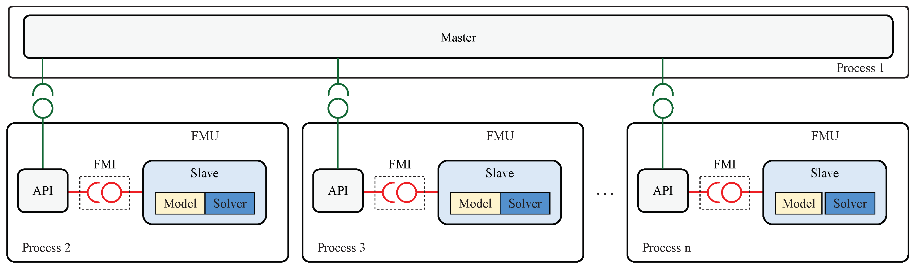
3. Co-Simulation Algorithm

In order to investigate electromagnetic transients caused by WPPs connected to larger power systems, for instance, it is mandatory to represent each WECS inside the wind farms in detail. Depending on the frequency range of the phenomena under analysis, it may be necessary to use a time-step in the order of microseconds. However, using traditional simulation approaches, these analyses are practically unfeasible due to the substantial digital requirements and high computational burden.

Traditionally, in electromagnetic transient (EMT) analysis, a specific area of interest in the system is meticulously modeled, while the surrounding areas are typically simplified using equivalent models [4]. Equivalent models offer the advantage of reduced computational overhead compared to detailed models. Nevertheless, as systems grow in complexity, the methods required to derive these equivalents also become more intricate [22]. One way to overcome the challenge of creating truly representative equivalent models for a system component is to utilize fully detailed models. However, simulating a multi-area system in such fine detail presents significant practical obstacles due to the considerably increased computational demands.

Through co-simulation techniques, multiple independent simulation tools, each one responsible for modeling a portion of the larger system, can be interconnected. This partitioning can substantially reduce simulation runtime, as each smaller subsystem can be modeled and simulated independently. The exchange of data and synchronization of the local simulation time for each simulator are managed by the co-simulation master algorithm. Since data exchange occurs via a communication network protocol, simulators can be physically distributed. This also facilitates the collaboration of different working groups in conducting simulations, bypassing limitations arising from the confidentiality of information and/or models [23]. The use of co-simulation techniques for analyzing multi-area systems, such as those in wind energy conversion, offers several additional advantages, as outlined below [23,24]:

• Independent development of models for each area by separate working groups with access to only essential information is feasible.
• The choice of simulation tools for each area becomes irrelevant, since data exchange occurs over a network using a standard protocol.
• Models can be kept private, if necessary, as only selected interface variables need to be shared with other simulators at runtime.
• Responsibilities related to model development and maintenance naturally divide among those with access to their respective information.
• The integration of new simulators or models can be achieved with ease.
• The distributed nature of co-simulation enables the sharing of the computational workload of the simulation.

The co-simulation enables the coupling between systems with multiple domains and stands as a flexible solution to overcome the complexity that exists in many practical engineering problems. It also allows subsystems to be solved with different simulation time steps and solvers, a condition that can be crucial to the integration of different domains [25].

3.1. Functional Mock-Up Interface

Co-simulation of coupled dynamic systems, where each subsystem is tackled by the most appropriate tool and has its own solution method, is a feature that has been shown to enable studies in heterogeneous systems. However, some incompatibilities and challenges could arise when performing the integration of subsystems modeled on different platforms.

In this context, with the objective of mitigating possible compatibility problems and establishing a standard in the implementation of co-simulations, the Functional Mock-up Interface was developed. FMI is an interface that aims at simplifying the creation, storage, exchange, and use of models in dynamic systems from different modeling and simulation tools [13]. The model of a subsystem that employs the FMI interface is called a Functional Mock-up Unit. Thus, through the standard defined by the FMI, it is ensured that an FMU will be compatible with all co-simulation tools that support this type of development.

The FMI standard is a solution to integrate subsystems originating from the same simulation environment or from different tools. In the first case, co-simulation is used only to share the computational burden, aiming at eliminating computational bottlenecks. However, in both cases, when exporting a subsystem according to the FMI standard, the generated FMU may contain, in addition to the model description, a dedicated mathematical solver. In this case, the solver is native to the platform used to export the FMU.

As illustrated in Figure 3, a simulation run is performed by means of the master–slave concept. Thus, the slave processes simulate each subsystem, while the master coordinates and synchronizes data transfer among them. The master algorithm, however, is not part of the FMI standard. The data exchange between the subsystems is usually carried out by means of an inter-process communication paradigm, such as message-passing interface (MPI). The definition of this communication layer is also not part of the FMI standard, and requires a proper API (Application Programming Interface) to establish and synchronize the communication among FMUs.

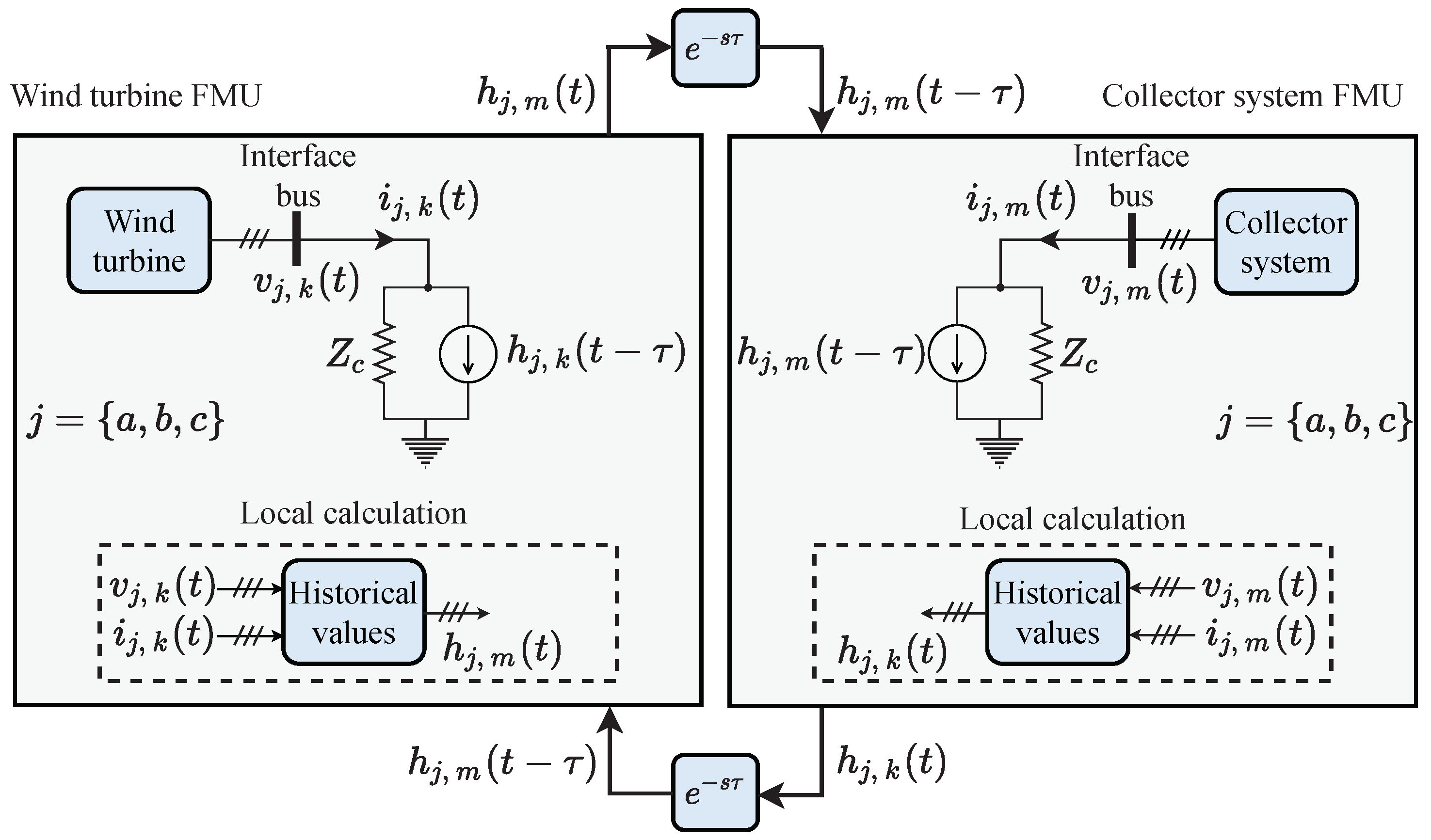
3.2. The Transmission Line Subsystem Coupling

The main objective of this work is to describe a large-scale co-simulation for a wind power generation system based on a WECS with type-4 topology. At the point of common coupling between each wind turbine and the collector grid of the WPP, the quantities involved are electrical in nature, that is, a set of three-phase voltages and currents. Due to the intrinsic characteristics of the control system, a wind turbine behaves as a current source while the collector grid plays the role of a voltage source. A simple communication protocol used in dynamic simulation programs would be, at each time step, to collect the currents from the wind turbines, distribute them appropriately along the collector system, and compute the voltages at terminal buses. Such voltages would then be redistributed to the wind turbine blocks that would be able to compute the currents in the next time step [26]. Such strategies, however, naturally introduce a time delay between voltages and currents, which may lead to numerically unstable conditions.

According to [3,27], the solution of the wave propagation equations through the transmission line (TL) allows for drawing the Bergeron model of the line shown in Figure 4, considering the frequency ${\omega }_o$ and the losses. This equivalent line model can be used to decouple the WECS from the collector network in a more natural and physically meaningful way. Thus, based on Figure 4, the currents $i_k\left(t\right)$ and $i_m\left(t\right)$ injected into the TL interface buses are given by

$$\begin{array}{cc}\hfill i_k\left(t\right)& =\frac{v_k\left(t\right)}{Z_c}+h_k(t-\tau )\hfill \end{array}$$

(9a)

$$\begin{array}{cc}\hfill i_m\left(t\right)& =\frac{v_m\left(t\right)}{Z_c}+h_m(t-\tau )\hfill \end{array}$$

(9b)

$$\begin{array}{cc}\hfill h_k\left(t\right)& =-\frac{v_m\left(t\right)}{Z_c}-i_m\left(t\right)\hfill \end{array}$$

(9c)

$$\begin{array}{cc}\hfill h_m\left(t\right)& =-\frac{v_k\left(t\right)}{Z_c}-i_k\left(t\right)\hfill \end{array}$$

(9d)

where $v_k\left(t\right)$ and $v_m\left(t\right)$ are, respectively, the terminal voltages at the TL interface buses, $h_k(t-\tau )$ and $h_m(t-\tau )$ are, respectively, the historical currents in the TL interface buses, $Z_c$ is the TL characteristic impedance, and $\tau$ is the travel time for a voltage or current wave to propagate from the TL terminals k to m. The historical terms $h_k(t-\tau )$ and $h_m(t-\tau )$ are calculated according to (9c) and (9d), respectively.

Since the above TL coupling is assumed to be a purely numerical artifice for interconnecting the WECS to the collector system, the travel time $\tau$ is assumed to be equal to the solution time-step $\Delta t$. It means that any event that occurs at one of the terminals will be perceived by the other end exactly one time-step later. Based on these assumptions, the coupling between the FMUs of a wind turbine and its respective connection bus with the collector grid is achieved as illustrated in Figure 4. The FMUs are characterized by their respective models and each subsystem comprises one of the terminals of the TL, according to the Bergeron model.

Therefore, during the co-simulation, only the historical current values of the interfacing TLs are exchanged between the FMUs. In addition, this configuration allows the execution of co-simulation on computational platforms with distributed resources as well. In such a case, a single process is dedicated to the solution of the collector grid and others to the wind turbines. In this work, the co-simulation algorithm sequence can be summarized as follows:

• At time $t=0$, the FMUs are initialized, including historical current values.
• Numerical integration of each FMU is performed.
• Historical values are calculated locally based on (9c) and (9d).
• The currents $h_{j,k}\left(t\right)$ and $h_{j,m}\left(t\right)$ are sent to the master, which, in turn, redistributes them to their associated subsystems.
• FMUs update their input values.
• Advance time $t\to t+\Delta t$.
• Steps (2) to (6) are repeated until the end of the simulation.

3.3. Communication Protocol

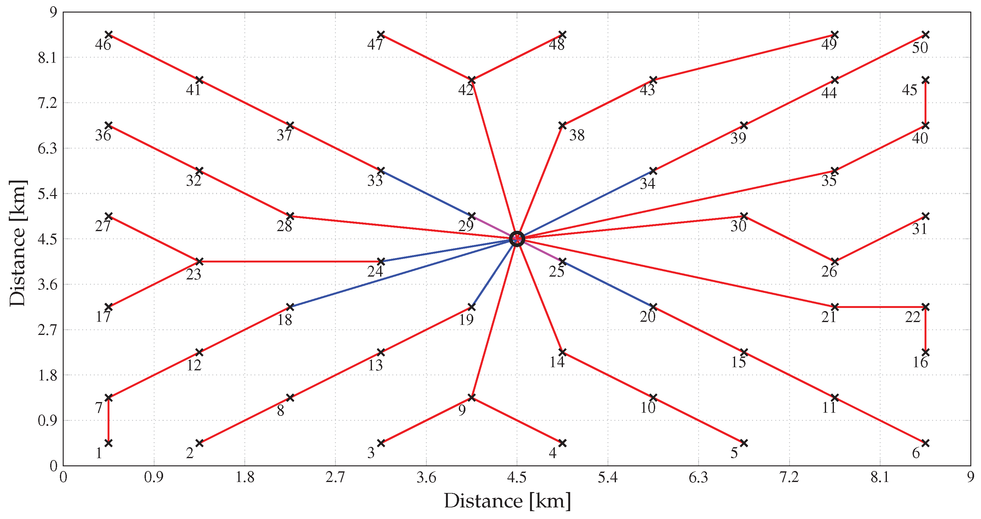
As previously emphasized, the co-simulation enables decoupling problems into distinct subsystems so that they can be solved independently. This framework naturally suggests the use of parallel computing to speed up the simulations. The adoption of parallel computing plays a vital role not only in the development of co-simulation but also in the feasibility of studying those problems that require high computational effort. There are different paradigms of parallel computing. However, in this work, the MPI standard is used. Through this paradigm, processes have their memory and communicate through explicit function calls for sending and receiving messages. Such processes can use end-to-end communication mechanisms or communicate collectively.

In the co-simulation of the wind energy generation systems proposed in this work, the problem is divided into processes dedicated to the solution of the electricity grid and others to the WECS. In this structure, simultaneously with the electrical network, the wind turbines are computed and, at the end of each integration step, every wind turbine communicates with the master process and vice versa. This characteristic enables the usage of collective communication routines to exchange data among subsystems.

Figure 5 shows a flowchart of the co-simulation master algorithm along with the communication pattern. At the beginning, all processes need to read all required parameters and be properly initialized. Afterwards, all subsystems perform an integration time-step simultaneously, and then calculate their historical current values $h_{j,k}\left(t\right)$ and $h_{j,m}\left(t\right)$. At the end of this step, all wind turbines send, at the same time, their historical values $h_{j,m}\left(t\right)$ to the master process. To perform this communication procedure, the gather function of the MPI standard is used. The simulation remains blocked until all messages are received by the master process. Next, the master process sends the historical currents $h_{j,k}\left(t\right)$, computed for the electrical grid subsystem, to all wind turbines. At this stage, for the sake of simplicity, the messages are sent through the bcast function of the MPI standard. Although there are more optimized ways to send the data from the electrical network to the wind generators, such as the scatter function, for instance, it was verified that this communication procedure incurs a negligible overhead. Finally, the subsystems are updated, enabling them to advance the time by a time-step and repeat the integration procedure until the end of the simulation is reached.

The co-simulation scheme detailed above will be evaluated in terms of two performance metrics: efficiency and speed-up. The master algorithm presented in Figure 5 can be analyzed from a computational and communication point of view, aiming at characterizing the timing needed to solve the subsystems and exchange data among them. Analyzing Figure 5, the total time $T_{total}$ spent to execute the co-simulation, using a parallel communication protocol, can be estimated by (10), where $T_{comp}$ is the maximum computing time among all processes; $T_{com}^{wecs}$ is the maximum communication time among wind turbines with the electrical grid; and $T_{com}^{grid}$ is the communication time of the electrical network with the wind turbines.

$$\begin{array}{c}\hfill T_{total}=T_{comp}+T_{com}^{wecs}+T_{com}^{grid}\end{array}$$

(10)

4. Test System

To evaluate the co-simulation strategy presented in this work, a wind farm of 500 $\mathrm{M}$$\mathrm{W}$ capacity was established. Figure 6 shows the topology of a 66 $\mathrm{k}$$\mathrm{V}$ offshore collector network with 50 wind turbines [28]. Each “×” mark in this figure represents the connection point of a wind turbine to the collector network. In addition, the central circle characterizes the offshore substation, here modeled as an infinite bus.

The cable segments in Figure 6 were simulated using the lumped parameters model of the transmission line, mainly because the longest section is smaller than $3.5$ $\mathrm{k}$$\mathrm{m}$. Detailed information about the network parameters and cable lengths can be found in

Table A8. Parameters of collector network (base values 100 $\mathrm{MVA}$ and 66 $\mathrm{k}\mathrm{V}$).

From	To	R [%]	X [%]	d [km]	From	To	R [%]	X [%]	d [km]
1	7	0.425	0.388	0.9	39	34	0.601	0.5487	1.2728
2	8	0.601	0.5487	1.2728	40	35	0.601	0.5487	1.2728
3	9	0.601	0.5487	1.2728	41	37	0.601	0.5487	1.2728
4	9	0.601	0.5487	1.2728	43	38	0.601	0.5487	1.2728
5	10	0.601	0.5487	1.2728	44	39	0.601	0.5487	1.2728
6	11	0.601	0.5487	1.2728	45	40	0.425	0.388	0.9
7	12	0.601	0.5487	1.2728	46	41	0.601	0.5487	1.2728
8	13	0.601	0.5487	1.2728	47	42	0.601	0.5487	1.2728
10	14	0.601	0.5487	1.2728	48	42	0.601	0.5487	1.2728
11	15	0.601	0.5487	1.2728	49	43	0.9503	0.8676	2.0125
12	18	0.601	0.5487	1.2728	50	44	0.601	0.5487	1.2728
13	19	0.601	0.5487	1.2728	9	51	1.5026	1.3718	3.182
15	20	0.601	0.5487	1.2728	14	51	1.0835	0.9893	2.2946
22	21	0.425	0.388	0.9	18	51	0.8343	1.059	2.6239
16	22	0.425	0.388	0.9	19	51	0.4525	0.5743	1.423
17	23	0.601	0.5487	1.2728	21	51	1.6184	1.4775	3.4271
27	23	0.601	0.5487	1.2728	24	51	0.4525	0.5743	1.423
23	24	0.85	0.776	1.8	25	51	0.1356	0.2399	0.6364
20	25	0.4047	0.5137	1.2728	28	51	1.0835	0.9893	2.2946
31	26	0.601	0.5487	1.2728	29	51	0.1356	0.2399	0.6364
32	28	0.601	0.5487	1.2728	30	51	1.0835	0.9893	2.2946
33	29	0.4047	0.5137	1.2728	34	51	0.607	0.7705	1.9092
26	30	0.601	0.5487	1.2728	35	51	1.6184	1.4775	3.4271
36	32	0.601	0.5487	1.2728	38	51	1.0835	0.9893	2.2946
37	33	0.601	0.5487	1.2728	42	51	1.5026	1.3718	3.182

(refer to Appendix A). In addition, the line models also do not consider shunt capacitance due to its negligible effect.

Figure 7 shows a detail of one of the wind energy conversion systems (WECSs). All units are identical to the Type-4 WECS shown in Figure 1. The parameters of each turbine are given in

Table A1. Parameters of wind turbine.

Parameter	Symbol	Value
Rated power	$P_{rated}$	10 $\mathrm{M}\mathrm{W}$
Optimal tip speed ratio	${\lambda }_{opt}$	10.59
Maximum power coefficient	$C_p^{max}$	0.47
WT diameter	D	180 $\mathrm{m}$
Initial wind speed	$V_w^{ini}$	2.96 $\mathrm{m}/\mathrm{s}$
Rated wind speed	$V_w^{rated}$	11.26 $\mathrm{m}/\mathrm{s}$
Maximum wind speed	$V_w^{max}$	25 $\mathrm{m}/\mathrm{s}$
Minimum turbine rotation	$n_T^{min}$	6.9 $\mathrm{rpm}$
Rated turbine rotation	$n_T^{rated}$	12.1 $\mathrm{rpm}$
Gearbox ratio	$N_g$	1:15
WT moment of inertia	$J_T$	$2.3552\times {10}^6$$\mathrm{k}\mathrm{g}·{\mathrm{m}}^2$
WT mechanical damping constant	$D_T$	$0.25\times {10}^6$$\mathrm{N}·\mathrm{m}·\mathrm{s}$

(refer to Appendix A). They were modeled using (1)–(4), and the coefficients $c_1$ to $c_9$ are given in

Table A2. Wind turbine dynamic model constants.

Constant	Value	Constant	Value
$c_1$	0.1828	$c_6$	9.1004
$c_2$	176.7595	$c_7$	13.0017
$c_3$	−2.0587	$c_8$	−0.0381
$c_4$	1.8007	$c_9$	−0.0340
$c_5$	1.1989

. The WT drives the PMSG, whose main parameters are given in

Table A3. Parameters of permanent magnet synchronous generator.

Parameter	Symbol	Value
Rated power	$P_b$	10 $\mathrm{M}\mathrm{W}$
Rated voltage	$V_b$	3 $\mathrm{k}\mathrm{V}$
Electric rated frequency	$f_b$	20 $\mathrm{Hz}$
Minimum rotation speed	$n_s^{min}$	90 $\mathrm{rpm}$
Maximum rotation speed	$n_s^{max}$	180 $\mathrm{rpm}$
Permanent magnet flux linkage	${\lambda }_m$	16.244 $\mathrm{Wb}$
Rotor moment of inertia	$J_m$	475.860 $\mathrm{k}\mathrm{g}·{\mathrm{m}}^2$
Stator winding resistance	$r_s$	8.945 $\mathrm{m}\mathsf{\Omega }$
Stator synchronous inductances	$L_{ds}=L_{qs}$	1.424 $\mathrm{m}\mathrm{H}$

.

Based on the preliminary tests, the power electronic converters impose a very large computational burden, even with the currently available co-simulation scheme. Thus, in order to prove only the potential of the co-simulation technique, the switched models of the converters have been replaced by average-based models [16]. The machine-side and grid-side converters are controlled in $dq$-reference frame. The MSC uses the rotor angle of the PMSG, while the GSC uses the angle obtained from a PLL [21], to synchronize their voltages and currents with the voltages of the generator terminals and the collector network, respectively. Notwithstanding, proportional–integral (PI) controllers were designed in $dq$-frame to regulate the currents synthesized by both converters, using the methodology presented in [20]. These controllers were embedded together with FMU models of the WT and PSMG. The main parameters of machine-side and grid-side converters are given, respectively, in

Table A4. Parameters of machine-side converter.

Parameter	Symbol	Value
PWM carrier wave frequency	$f_{s1}$	5 $\mathrm{kHz}$
Series filter resistance	$R_g$	51 $\mathrm{m}\mathsf{\Omega }$
Series filter inductance	$L_g$	5 $\mathrm{m}\mathrm{H}$
DC link average voltage	$V_{dc}$	10 $\mathrm{k}\mathrm{V}$
DC link capacitance	$C_{dc}$	400 $\mathsf{\mu }\mathrm{F}$

and

Table A5. Parameters of grid-side converter.

Parameter	Symbol	Value
PWM carrier wave frequency	$f_{s2}$	5 $\mathrm{kHz}$
Series filter resistance	$R_r$	51 $\mathrm{m}\mathsf{\Omega }$
Series filter inductance	$L_r$	5 $\mathrm{m}\mathrm{H}$
Shunt filter resistance	$R_f$	6 $\mathsf{\Omega }$
Shunt filter capacitance	$C_f$	98 $\mathsf{\mu }\mathrm{F}$

, while the gains of the current controllers can be found in

Table A6. Gains of the current controllers of the MSC and GSC.

Side	Parameter	Symbol	Value
MSC	proportional gain	$k_{p,i}$	1.2890 $\mathrm{V}/\mathrm{A}$
	Integral gain	$k_{i,i}$	12.8473 $\mathrm{V}/\mathrm{A}\mathrm{s}$
GSC	proportional gain	$k_{p,i}$	1.0 $\mathrm{V}/\mathrm{A}$
	Integral gain	$k_{i,i}$	25.5 $\mathrm{V}/\mathrm{A}\mathrm{s}$

.

In addition, an external speed controller maximizes the power captured from the wind by regulating the turbine rotation speed through the control of the power drained from the PMSG by the MSC [29]. This maximum power point tracking (MMPT) algorithm uses (4) to calculate the reference rotation speed so that maximum power is extracted from the wind turbine. At the output terminals of the interface converter, an outer voltage controller regulates the amount of active power that the GSC injects into the collector network to control the DC link voltage of the back-to-back converter. These two external controllers were designed with time constants one decade higher than the time constants of the inner current controllers [20] and their gains can be found in

Table A7. Gains of the outer controllers of the MSC and GSC.

Side	Parameter	Symbol	Value
MSC	proportional gain	$k_{p,\omega }$	$1.1029\times {10}^6\mathrm{A}/\mathrm{rad}/\mathrm{s}$
(WT rotation)	Integral gain	$k_{i,\omega }$	$0.5257\times {10}^6\mathrm{A}/\mathrm{rad}$
GSC	proportional gain	$k_{p,dc}$	$24.8801\times {10}^{-6}\mathrm{A}/\mathrm{V}$
(DC link voltage)	Integral gain	$k_{i,dc}$	$3.34\times {10}^{-3}\mathrm{A}/\mathrm{V}\mathrm{s}$

.

The interface between each WECS and the collector system comprises an ideal transmission line Bergeron-equivalent model, as depicted in Figure 4. In this way, only historical current values are exchanged by subsystems at each simulation time-step. Moreover, in the conducted co-simulations, the system is statically partitioned so that each processing unit has the same number of WECSs to handle.

It is important that the value of $Z_c$ be chosen carefully to avoid a sharp mismatch between the input and output signals, resulting in an attenuation in the quantities involved in the coupling or even numerical instability. A proper choice for the characteristic impedance of transmission line link is an issue still under investigation. Simulation tests indicated that a value equal to the base impedance of the collector network made the choice empirically adequate. The base parameters for WECS units can be found in

Table 1. Base parameters of the system.

Parameter	Symbol	Value
PMSG base power	$S_B$	10 $\mathrm{M}\mathrm{W}$
PMSG base voltage	$V_{B2}$	3 $\mathrm{k}\mathrm{V}$
Collector grid base voltage	$V_{B1}$	66 $\mathrm{k}\mathrm{V}$
Time step	$\Delta t$	50 $\mathsf{\mu }\mathrm{s}$

.

5. Simulation Results

The results obtained through co-simulation in a distributed computing architecture were compared with the ones obtained with a single core simulation, so accuracy and speed-up gains could be measured. The computational platform used for the simulations consisted of computing nodes with two Intel Quad-Core Xeon E5620 processors ( $2.40$ GB, 12 MB cache, 12 GB RAM memory DDR3 1066 MHz) interconnected by means of a Gigabit Ethernet network.

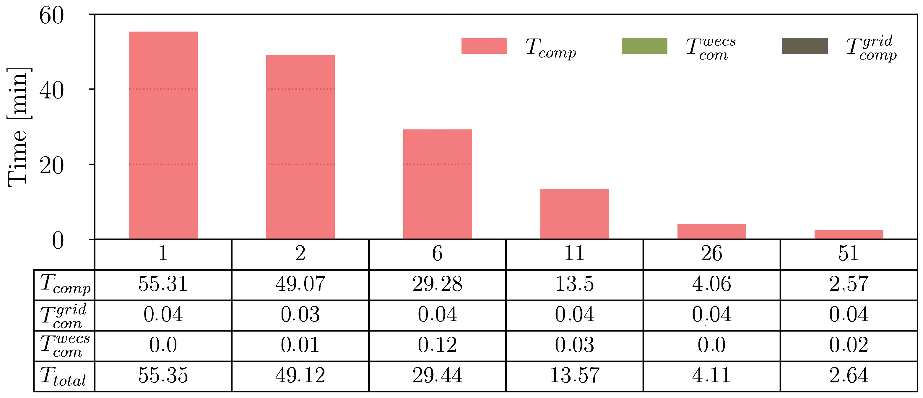
5.1. Computational Performance

In the first case, the WPP with 50 wind turbine units is simulated for 100 $\mathrm{m}$$\mathrm{s}$. The parallelization was carried out so that the master process, in addition to coordinating and synchronizing the co-simulation, also computes the collector grid. Furthermore, the distribution of wind turbines among computational processes was designed to balance the computational load to be attributed to each process.

Figure 8 shows the timings obtained with proposed simulations. The timings are displayed as a function of the number of partitions. It is important to emphasize that a simulation of the proposed test system as a whole, i.e., a monolithic system, by a single solver is simply not viable. Therefore, the time bar for a single process in Figure 8 characterizes the co-simulation performed by a single computing process. This is the timing that is taken as reference for the subsequent comparisons.

One can observe that as the number of partitions increases, the simulation time is significantly reduced. It can be inferred that the global solution time of the co-simulation is strongly related to the number of wind turbines solved per process. One can also observe that the overhead time due to the inter-process communication can be considered negligible.

In order to evaluate the computational performance, two indices are usually considered, namely, speed-up $\mathcal{S}$ and efficiency $\mathcal{E}$ [30]. The speed-up $\mathcal{S}$ is defined as the ratio between the sequential $T_s$ and parallel $T_p$ timings, while the efficiency corresponds to the ratio between the speed-up $\mathcal{S}$ and the number of processes p.

As one can observe, the presented co-simulation strategy with 51 partitions achieves a speed-up of 21 with respect to the sequential one, as shown in Figure 9. In addition, Figure 9 also shows that, as the number of partitions increases, a saturation in the speed-up is observed along with a reduction in the efficiency.

The performance analysis shows that the co-simulation technique is a suitable alternative that can enable studies in those systems with high computational demand. Moreover, one can also conclude that, with an adequate partitioning scheme of the total computational load, the proposed co-simulation algorithm is able to considerably accelerate the required power system computations.

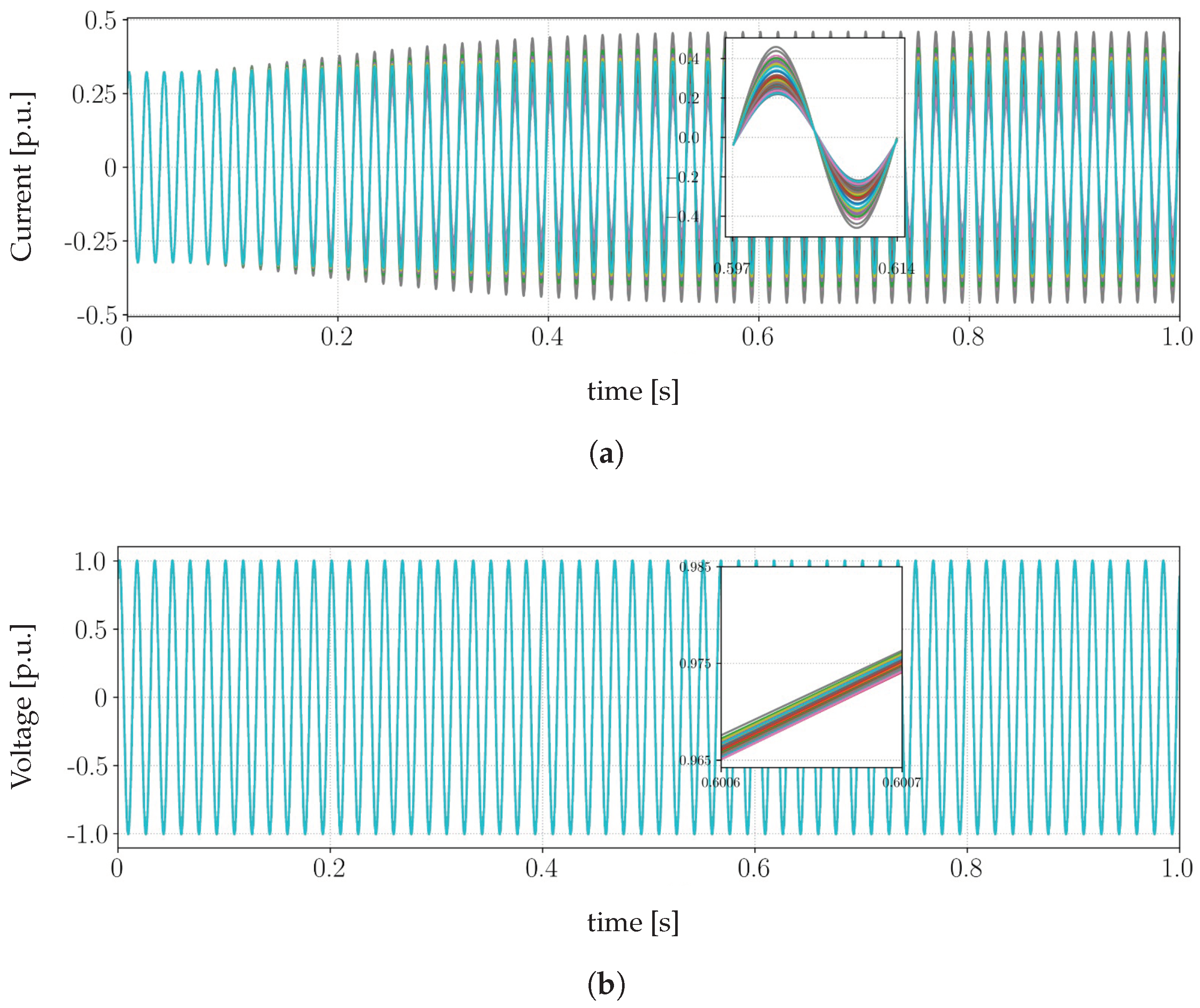
5.2. Voltage Dip at the Collecting Substation

In order to demonstrate the electrical performance of the WPP calculated by means the co-simulation, the system operates in steady state, when at $t=50 \mathrm{m}\mathrm{s}$, a dip of 50% of the nominal voltage is simulated in the collecting substation. The voltage reduction is sustained for 100 $\mathrm{m}$$\mathrm{s}$, while the wind power converted by the turbine remains constant. To illustrate the results, the dynamic behavior of the wind turbine connected to bus 27 of the collector network is discussed next.

Figure 10a depicts the $dq$-components of the voltage at the primary winding of the step-up interface transformer. One can observe that the instantaneous voltage dip induces damped numerical oscillations, introduced by the transmission line Bergeron model. On the other hand, Figure 10b shows the current flowing through the grid-side LC filter. As expected, during the disturbance in the system, the current injected by the WECS increases as the wind power is kept constant, as shown in Figure 10c.

Figure 11a and Figure 11b show, respectively, the currents and voltages in the coupling between the wind turbine and the electrical grid. Once again, due to the instantaneous voltage dip, numerical oscillations are excited at the moment of the disturbance. After a few time-steps, the lower frequency range phenomena are properly tracked by the co-simulation.

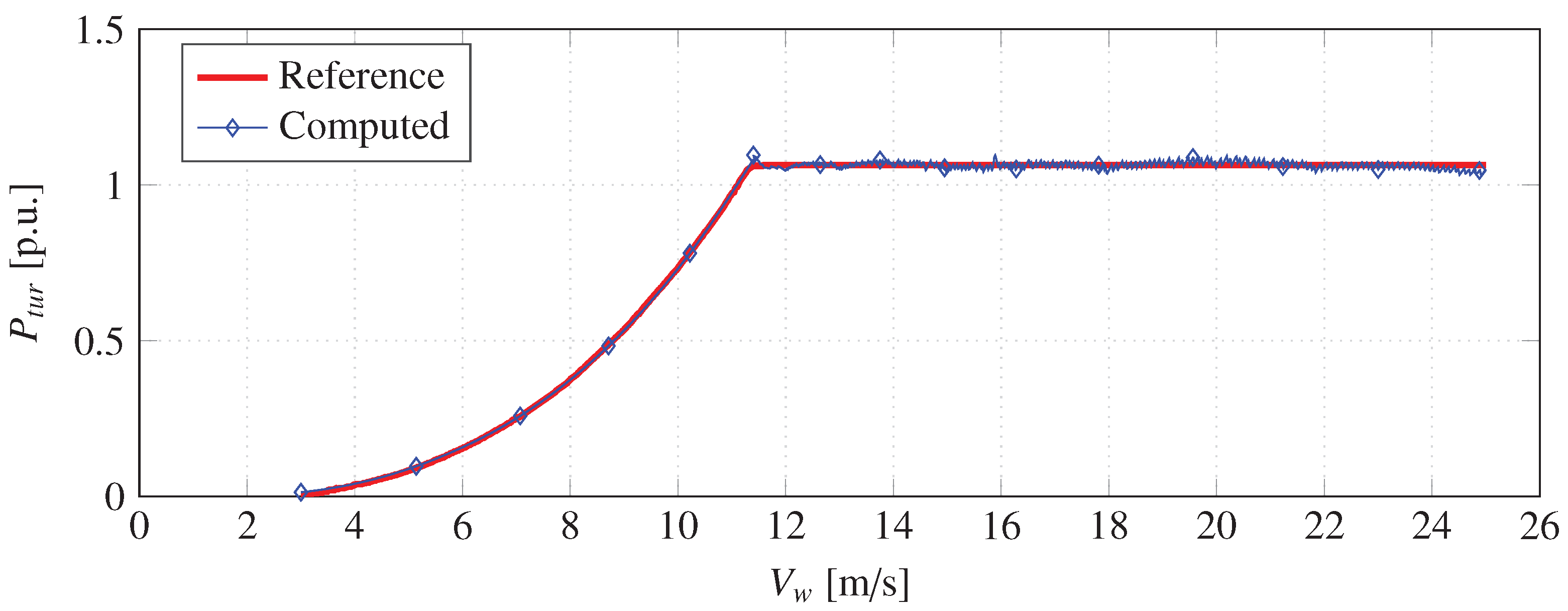
5.3. Wind Velocity Variation

To assess the electromechanical performance of the WPP, every WECS unit is subjected to a wind speed velocity change. At the beginning of the simulation, the system operates in steady state, and at $t=50 \mathrm{m}\mathrm{s}$, the wind speed randomly changes in the range of ±1 $\mathrm{m}$/$\mathrm{s}$. The primary objective here is to demonstrate that parallel-processed co-simulation allows for extended simulation periods within a practical execution time frame while ensuring that individual WECS controllers function as intended.

Figure 12a illustrates the response of wind turbine velocities to variations in wind speed, while Figure 12b displays the instantaneous active power injected into the collector system by all 50 turbines at their respective interface buses. It is evident that the active power response in each wind conversion system exhibits a first-order behavior, aligning with the design principles of the GSC current control loop.

The instantaneous currents, as depicted in Figure 13a, also respond to changes in wind speed, increasing or decreasing in accordance with each turbine’s fluctuations. Meanwhile, Figure 13b displays the instantaneous voltages at the interface buses. It is worth noting that the amplitudes remain practically constant, and the angular lags are minimal. This is primarily due to the unity power factor control, which keeps currents low at these points, and the short electrical distances between nodes in the collector system.

Considering the computational speed-up achieved through co-simulation, it took an average of 60 s to simulate 1 s of the system. In contrast, a monolithic simulation would require approximately 1200 min (20 h).

6. Conclusions

This paper presented the simulation of wind power plants by means of co-simulation techniques. Results demonstrated the effectiveness of the proposed co-simulation technique as an alternative to overcome the computational bottlenecks usually faced in the simulation of electrical power systems with high penetration of renewable generation typically interfaced to the network by means of power-electronics-based converters.

Two main contributions can be pointed out in the present work. Firstly, the Functional Mock-up Interface (FMI) standard was used to implement different parts of the system, which, in addition to enabling different tools to be coupled in a single simulation, also guarantees the intellectual property of the developed models. Furthermore, this approach allows one to promptly share computational burden among several processing units, which may drastically improve the total simulation computing time. For achieving the decoupling of the subsystems, fictitious ideal transmission lines were used with traveling time equal to the simulation time-step.

Another contribution of the present work can be identified in the use of a high-performance computing platform combined with Functional Mock-up Units (FMUs) for modeling and simulating electrical power systems. Here, the co-simulation master algorithm was implemented in Python and relied on the message-passing interface (MPI) to synchronize and coordinate the distributed co-simulation.

The computational performance of the proposed co-simulation technique was evaluated with a wind power plant with 50 wind turbines. Splitting the computational burden along with the subsystems resulted in a simulation roughly 20 times faster than its sequential counterpart, while keeping an efficiency of approximately 40%, when 51 processing units were employed.

References

- Issacs, A. Simulation technology: The evolution of power system modeling. IEEE Power Energy Mag. 2017, 15, 88–102. [Google Scholar] [CrossRef]
- Kundur, P.; Paserba, J.; Ajjarapu, V.; Andersson, G.; Bose, A.; Canizares, C.; Hatziargyriou, N.; Hill, D.; Stankovic, A.; Taylor, C.; et al. Definition and classification of power system stability IEEE/CIGRE joint task force on stability terms and definitions. IEEE Trans. Power Syst. 2004, 19, 1387–1401. [Google Scholar]
- Watson, N.; Arrillaga, J. Power Systems Electromagnetic Transients Simulation; IET Power and Energy Series; The Institution of Engineering and Technology (IET): Bodmin, UK, 2003; Volume 39. [Google Scholar]
- Campello, T.; Varricchio, S.; Taranto, G. Representation of multiport rational models in an electromagnetic transients program: Networks with lumped and distributed parameters. Electr. Power Syst. Res. 2020, 178, 106029. [Google Scholar] [CrossRef]
- Hussein, D.N.; Matar, M.; Iravani, R. A wideband equivalent model of type-3 wind power plants for EMT studies. IEEE Trans. Power Deliv. 2016, 31, 2322–2331. [Google Scholar] [CrossRef]
- Gomes, C.; Thule, C.; Broman, D.; Larsen, P.G.; Vangheluwe, H. Co-simulation: State of the art. arXiv 2017, arXiv:1702.00686. [Google Scholar]
- Andersson, C. Methods and Tools for Co-Simulation of Dynamic Systems with the Functional Mock-up Interface. Ph.D. Thesis, Lund University, Lund, Sweden, 2016. [Google Scholar]
- Shu, D.; Wei, Y.; Dinavahi, V.; Wang, K.; Yan, Z.; Li, X. Cosimulation of Shifted-Frequency/Dynamic Phasor and Electromagnetic Transient Models of Hybrid LCC-MMC DC Grids on Integrated CPU–GPUs. IEEE Trans. Ind. Electron. 2019, 67, 6517–6530. [Google Scholar] [CrossRef]
- Rupasinghe, J.; Filizadeh, S.; Gole, A.M.; Strunz, K. Multi-rate co-simulation of power system transients using dynamic phasor and EMT solvers. J. Eng. 2020, 2020, 854–862. [Google Scholar] [CrossRef]
- Tremblay, O.; Rimorov, D.; Gagnon, R.; Fortin-Blanchette, H. A multi-time-step transmission line interface for power hardware-in-the-loop simulators. IEEE Trans. Energy Convers. 2019, 35, 539–548. [Google Scholar] [CrossRef]
- Le-Huy, P.; Sybille, G.; Giroux, P.; Loud, L.; Huang, J.; Kamwa, I. Real-time electromagnetic transient and transient stability co-simulation based on hybrid line modelling. IET Gener. Transm. Distrib. 2017, 11, 2983–2990. [Google Scholar] [CrossRef]
- Niemeyer, G.; Slotine, J.J. Stable adaptive teleoperation. IEEE J. Ocean. Eng. 1991, 16, 152–162. [Google Scholar] [CrossRef]
- Modelica Association Project FMI. The Leading Standard to Exchange Dynamic Simulation Models. 2021. Available online: https://fmi-standard.org (accessed on 1 January 2021).
- The Modelica Association. Modelica Language. 2021. Available online: https://modelica.org/language (accessed on 1 February 2021).
- Yaramasu, V.; Wu, B.; Sen, P.C.; Kouro, S.; Narimani, M. High-power wind energy conversion systems: State-of-the-art and emerging technologies. Proc. IEEE 2015, 103, 740–788. [Google Scholar] [CrossRef]
- Yazdani, A.; Iravani, R. Voltage-Sourced Converters in Power Systems: Modeling, Control, and Applications; Wiley-IEEE: Hoboken, NJ, USA, 2010. [Google Scholar]
- Slootweg, J.G.; Polinder, H.; Kling, W.L. Representing wind turbine electrical generating systems in fundamental frequency simulations. IEEE Trans. Energy Convers. 2003, 18, 516–524. [Google Scholar] [CrossRef]
- Jonkman, J.; Butterfield, S.; Musial, W.; Scott, G. Definition of a 5-MW Reference Wind Turbine for Offshore System Development; Technical Report; National Renewable Energy Lab. (NREL): Golden, CO, USA, 2009. [Google Scholar]
- Krause, P.; Wasynczuk, O.; Sudhoff, S. Analysis of Electric Machinery and Drive Systems, 2nd ed.; IEEE Press Series on Power Engineering; IEEE Press: New York, NY, USA, 2002. [Google Scholar]
- Paulo, M.S.; Almeida, A.O.; Almeida, P.M.; Barbosa, P.G. Control of an Offshore Wind Farm Considering Grid-Connected and Stand-Alone Operation of a High-Voltage Direct Current Transmission System Based on Multilevel Modular Converters. Energies 2023, 16, 5891. [Google Scholar] [CrossRef]
- Rodriguez, P.; Teodorescu, R.; Candela, I.; Timbus, A.V.; Liserre, M.; Blaabjerg, F. New positive-sequence voltage detector for grid synchronization of power converters under faulty grid conditions. In Proceedings of the 37th IEEE Power Electronics Specialists Conference, Jeju, Republic of Korea, 18–22 June 2006; IEEE: Hoboken, NJ, USA, 2006; pp. 1–7. [Google Scholar]
- Hussein, D.N.; Matar, M.; Iravani, R. A type-4 wind power plant equivalent model for the analysis of electromagnetic transients in power systems. IEEE Trans. Power Syst. 2012, 28, 3096–3104. [Google Scholar] [CrossRef]
- Palensky, P.; Cvetković, M.; Keviczky, T. Intelligent Integrated Energy Systems: The PowerWeb Program at TU Delft; Springer: Cham, Switzerland, 2019. [Google Scholar]
- Silva, L.T.F.W. Modeling and Co-Simulation of Wind Energy Generation Systems. Master’s Thesis, Universidade Federal de Juiz de Fora, Juiz de Fora, Brazil, 2020. (In Portuguese). [Google Scholar]
- Theodoro, T.S. Hybrid Simulation in the Time Domain of Electromechanical and Electromagnetic Transients: Integration of a Wind Turbine Based on Doubly Fed Induction Generator. Master’s Thesis, Universidade Federal de Juiz de Fora, Juiz de Fora, Brazil, 2016. (In Portuguese). [Google Scholar]
- Theodoro, T.S.; Tomim, M.A.; Barbosa, P.G.; Lima, A.C.S.; de Barros, M.T.C. A flexible co-simulation framework for penetration studies of power electronics based renewable sources: A new algorithm for phasor extraction. Int. J. Electr. Power Energy Syst. 2019, 113, 419–435. [Google Scholar] [CrossRef]
- Arrillaga, J.; Arnold, C. Computer Analysis of Power Systems; Wiley: New York, NY, USA, 1990. [Google Scholar]
- Cabral, V.A.; Marliere, F.T.; Panoeiro, F.F.; Rebello, G.S.; Oliveira, L.W.; da Silva Junior, I.C. Wind Farm Collector System Optimization via Modified Bat-Inspired Algorithm. In Proceedings of the 13th Latin-American Congress on Electricity Generation and Transmission-Clagtee, Santiago, Chile, 20–23 October 2019. [Google Scholar]
- Wu, B.; Lang, Y.; Zargari, N.; Kouro, S. Power Conversion and Control of Wind Energy Systems; John Wiley & Sons: Hoboken, NJ, USA, 2011; Volume 76. [Google Scholar]
- Grama, A.; Kumar, V.; Gupta, A.; Karypis, G. Introduction to Parallel Computing; Pearson Education: London, UK, 2003. [Google Scholar]
Disclaimer/Publisher’s Note: The statements, opinions and data contained in all publications are solely those of the individual author(s) and contributor(s) and not of MDPI and/or the editor(s). MDPI and/or the editor(s) disclaim responsibility for any injury to people or property resulting from any ideas, methods, instructions or products referred to in the content. |
© 2023 by the authors. Licensee MDPI, Basel, Switzerland. This article is an open access article distributed under the terms and conditions of the Creative Commons Attribution (CC BY) license (https://creativecommons.org/licenses/by/4.0/).