
Comparison of Extreme Wind and Waves Using Different Statistical Methods in 40 Offshore Wind Energy Lease Areas Worldwide


 ,
,  ,
, 

Abstract
:1. Introduction
1.1. Background and Motivation
1.2. Literature Review
1.3. Research Objectives and Novelties
1.4. Novelties
2. Methodology
2.1. Criteria for Choosing Offshore Wind Lease Areas
2.2. Source of Raw Data
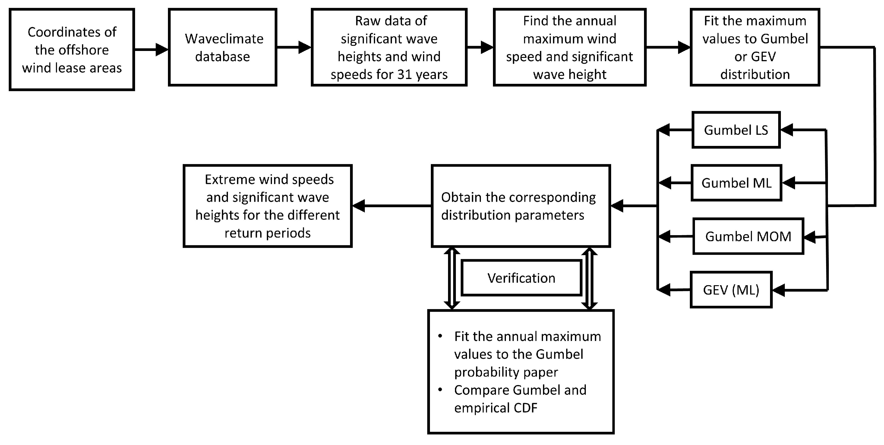
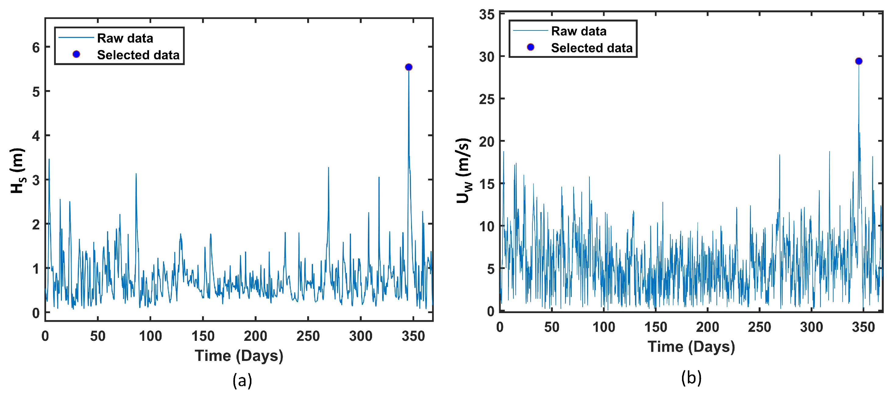
2.3. Block-Maxima Approach
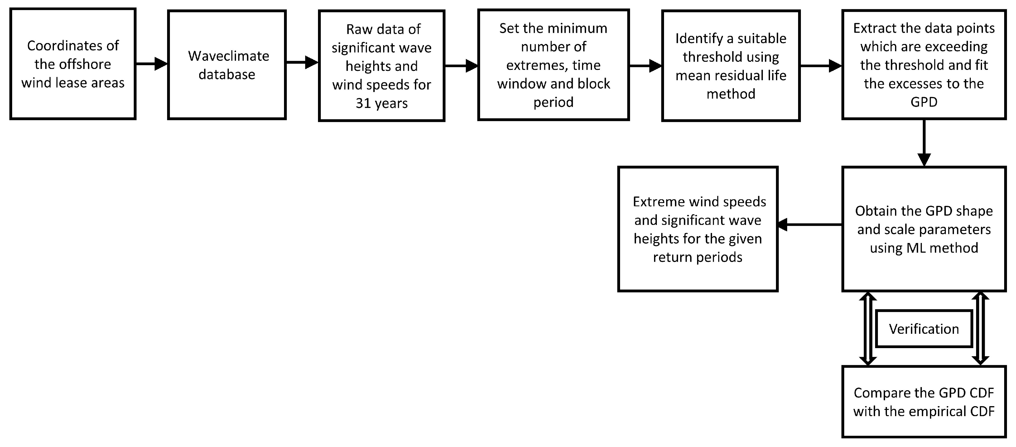
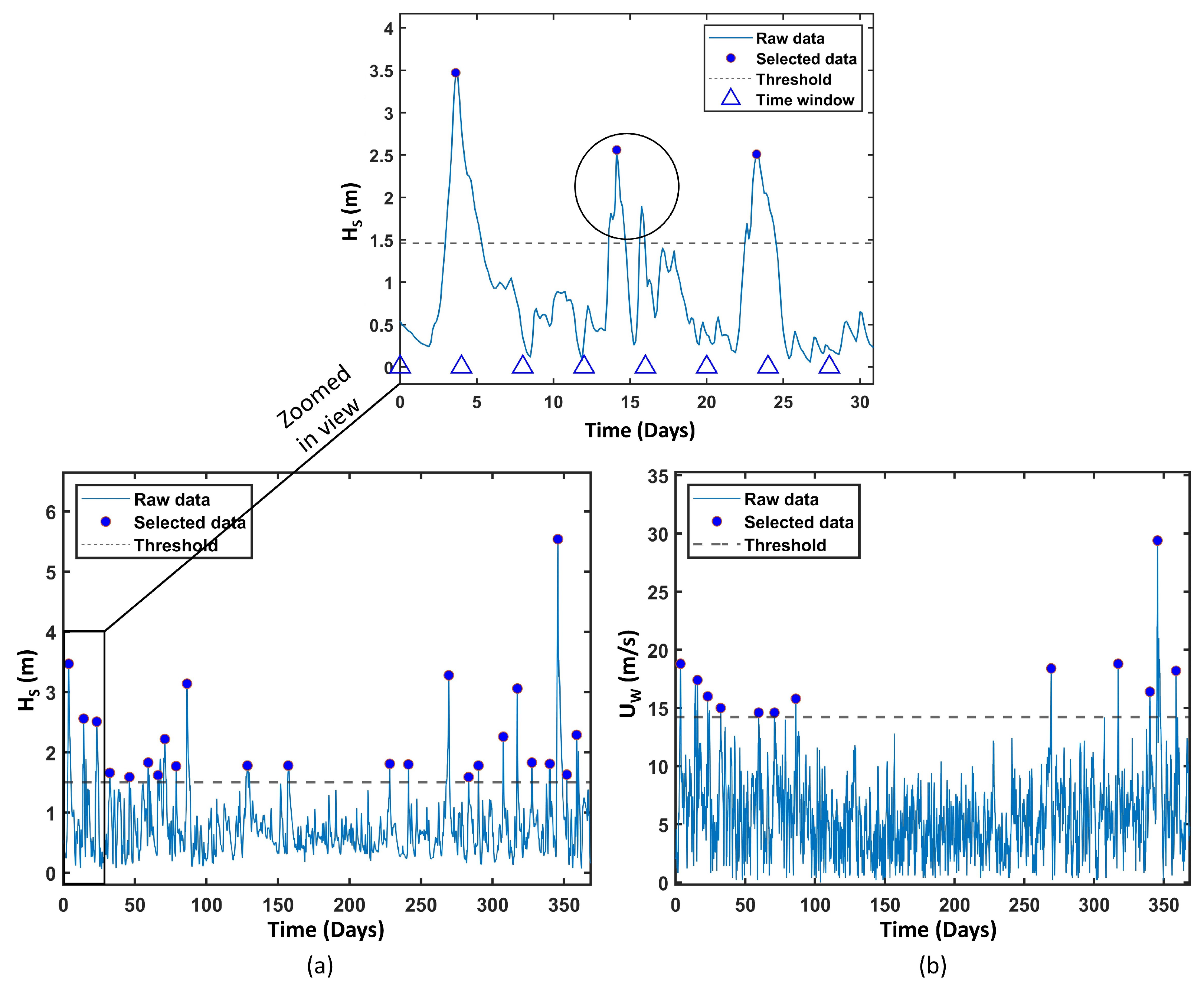
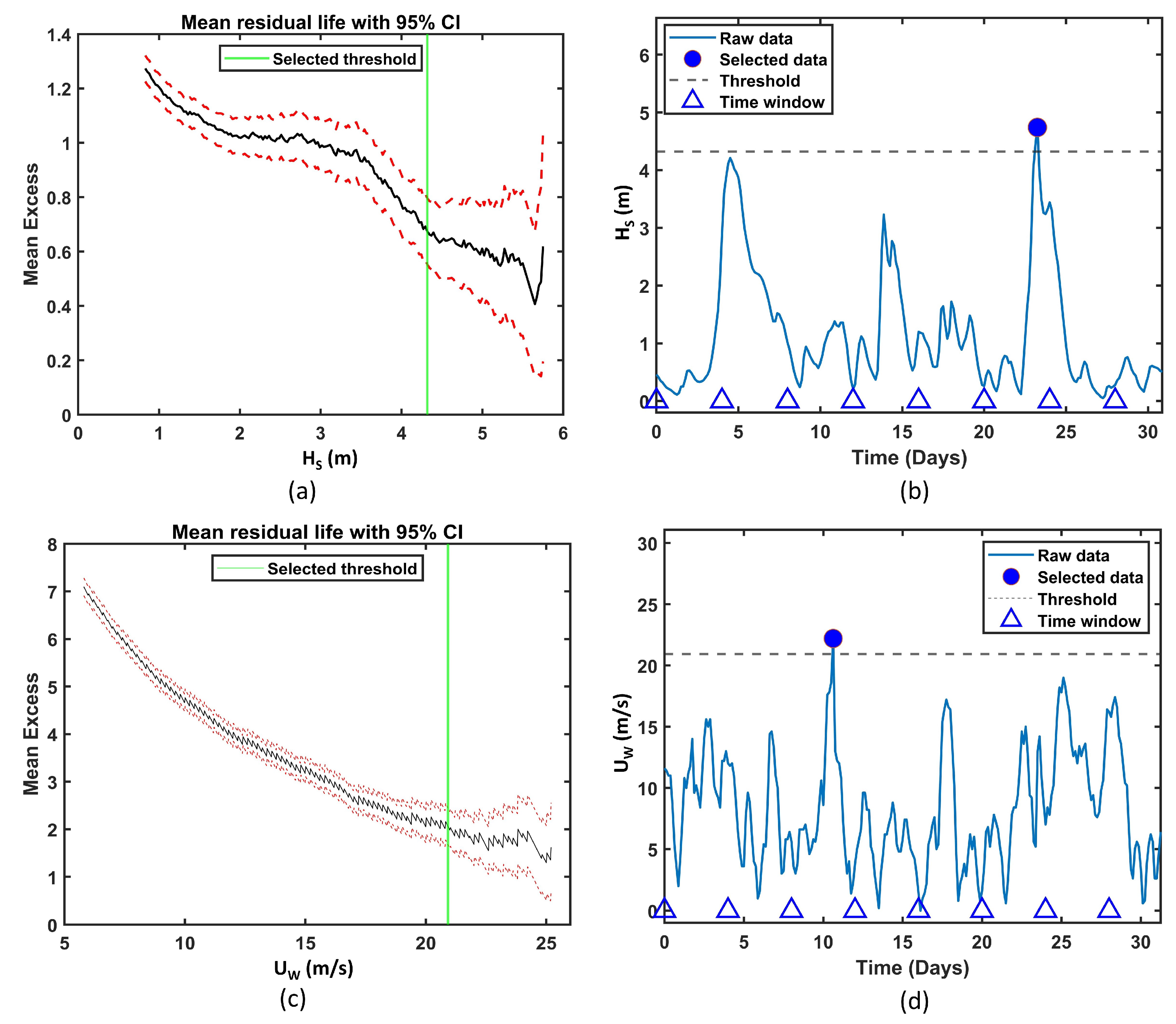
2.4. POT Approach
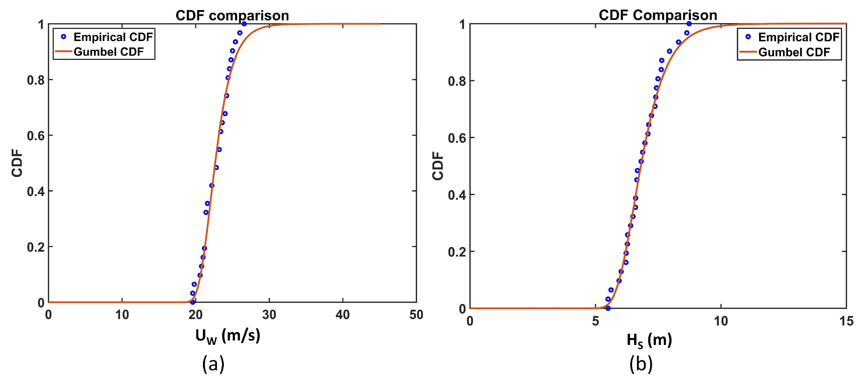
2.5. Verification
2.6. Assumptions and Limitations
3. Results and Discussion
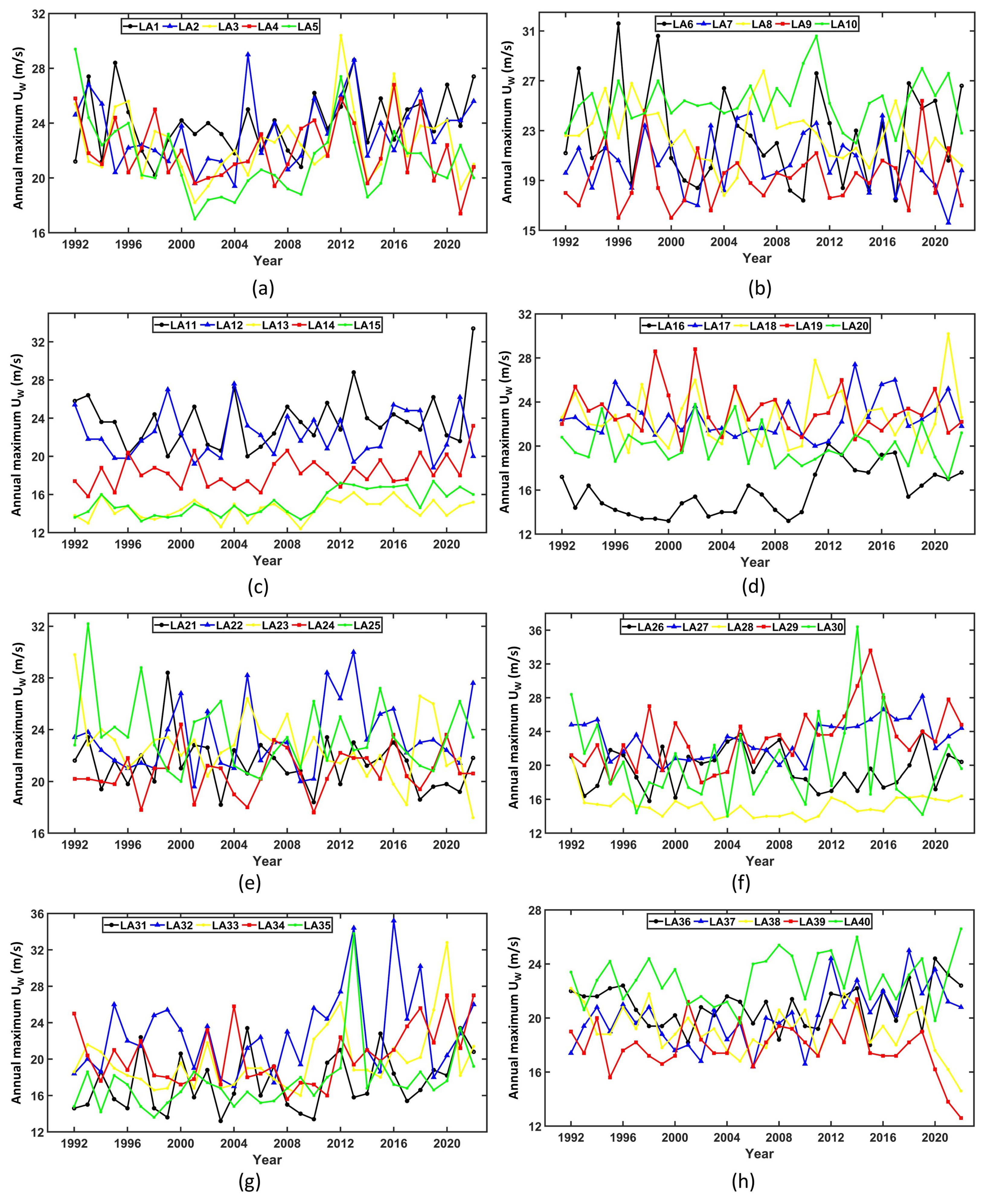
3.1. Block-Maxima Approach
3.2. POT Approach
3.3. Comparison of Extreme Values from the Block-Maxima and POT Approaches
4. Conclusions
- LA30 (Huaneng Hainan Wenchang I, China) recorded the outright highest annual maximum of 36.2 m/s, while LA10 (Allan array, Canada) recorded the highest mean annual maximum of 25.2 m/s.
- LA25 (GoliatVIND, Norway) recorded the highest mean annual maximum of 9.85 m, as well as the outright highest annual maximum of 14.2 m.
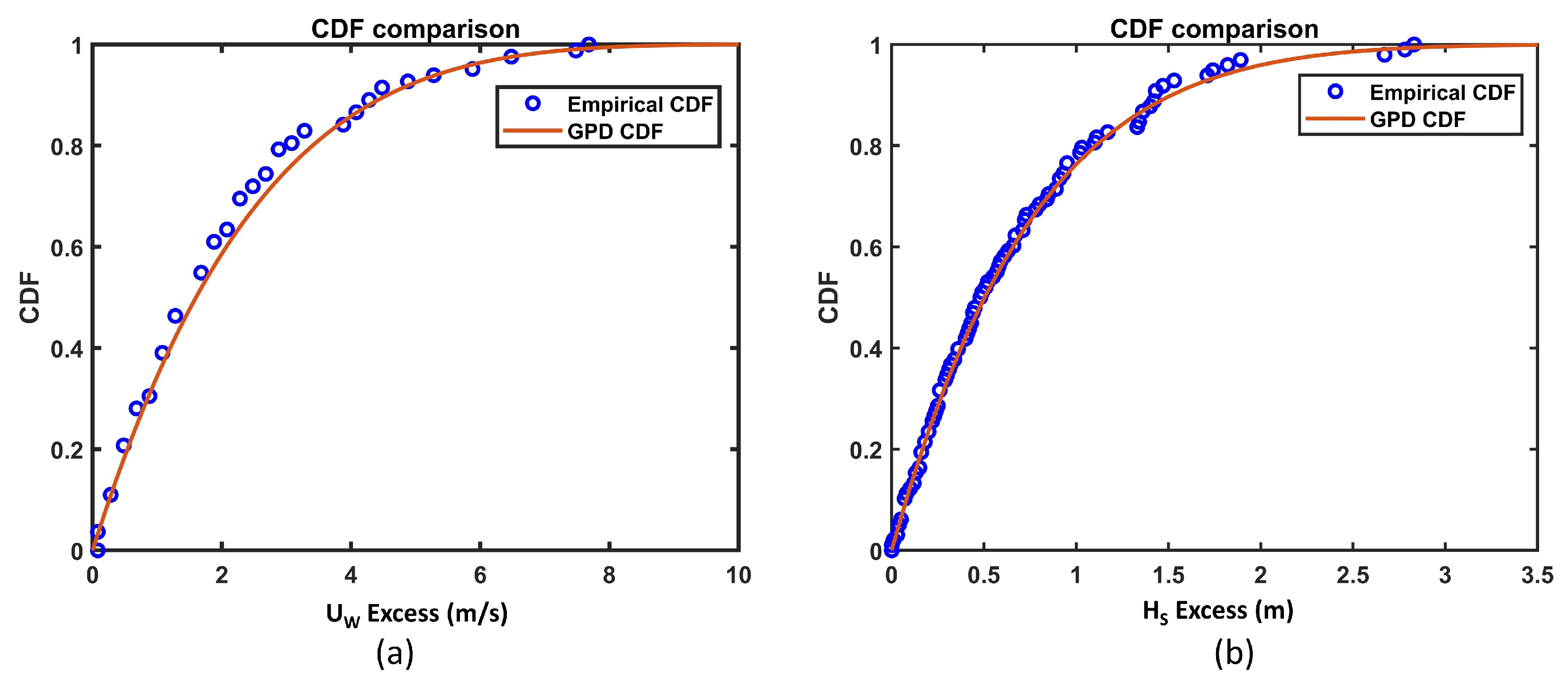
- The GPD CDF and Gumbel CDF showed good agreement with the empirical CDF for both the and values for all of the sites.
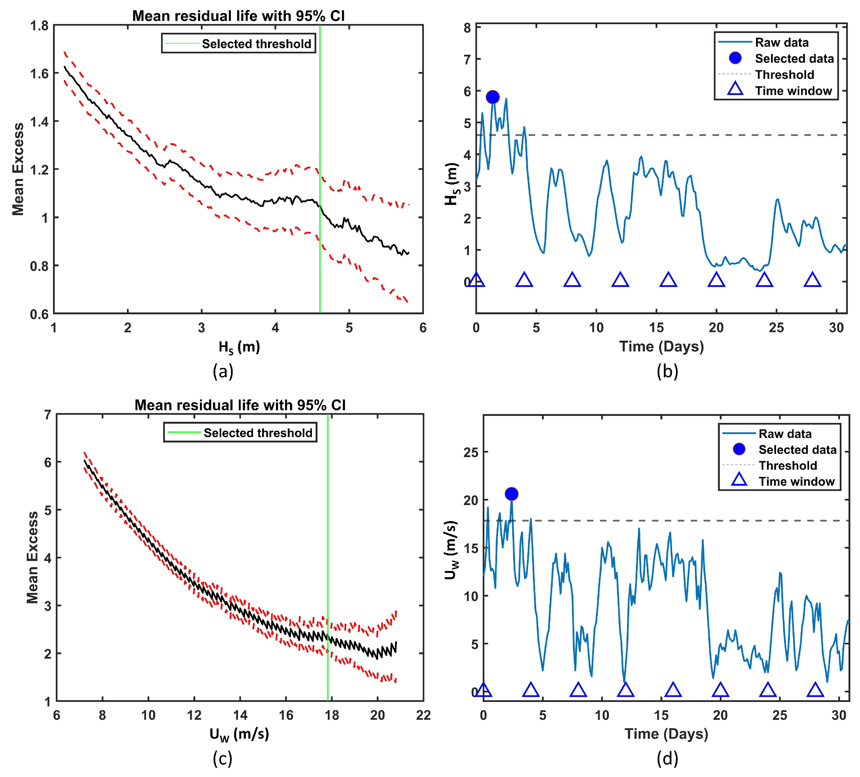
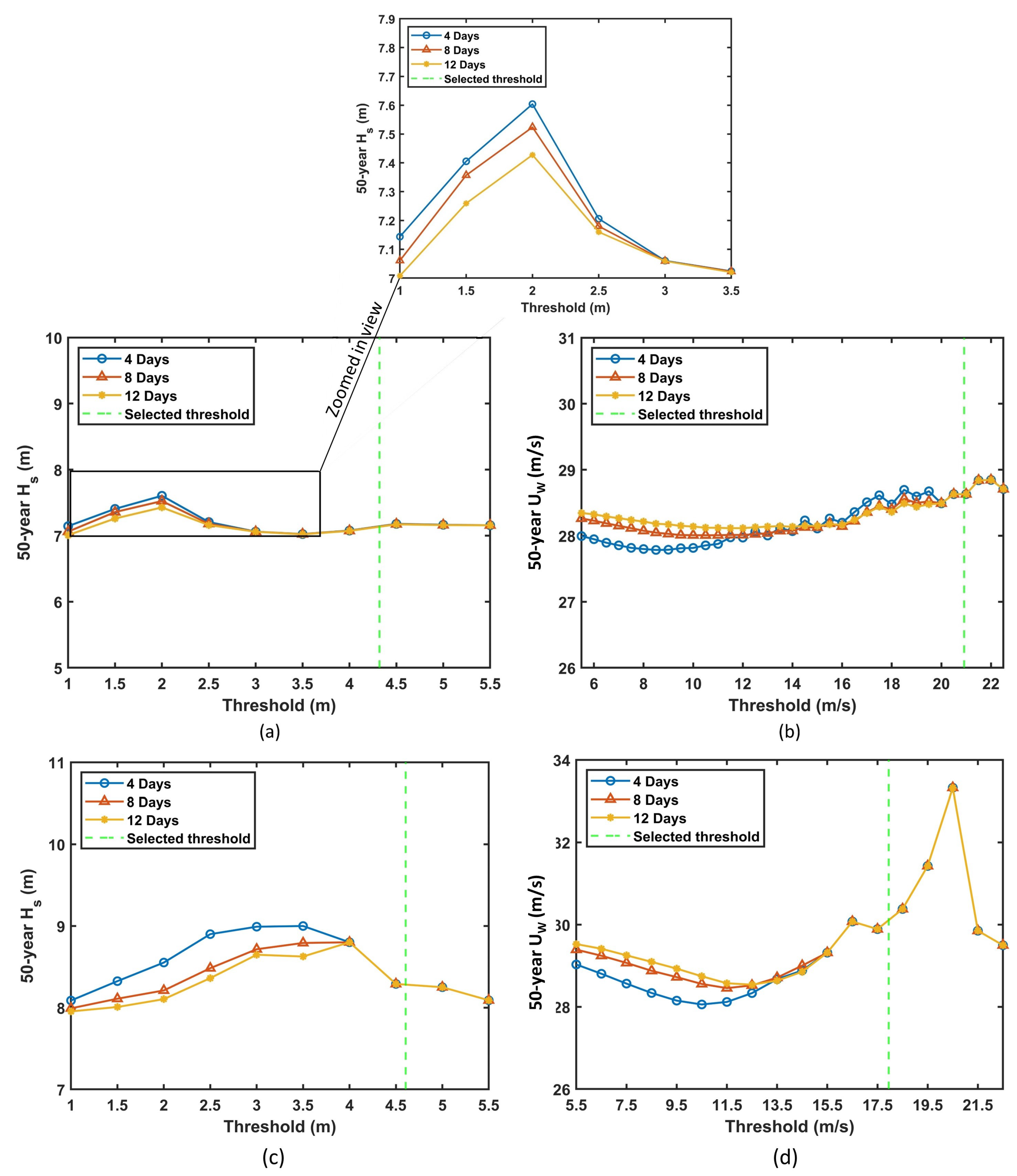
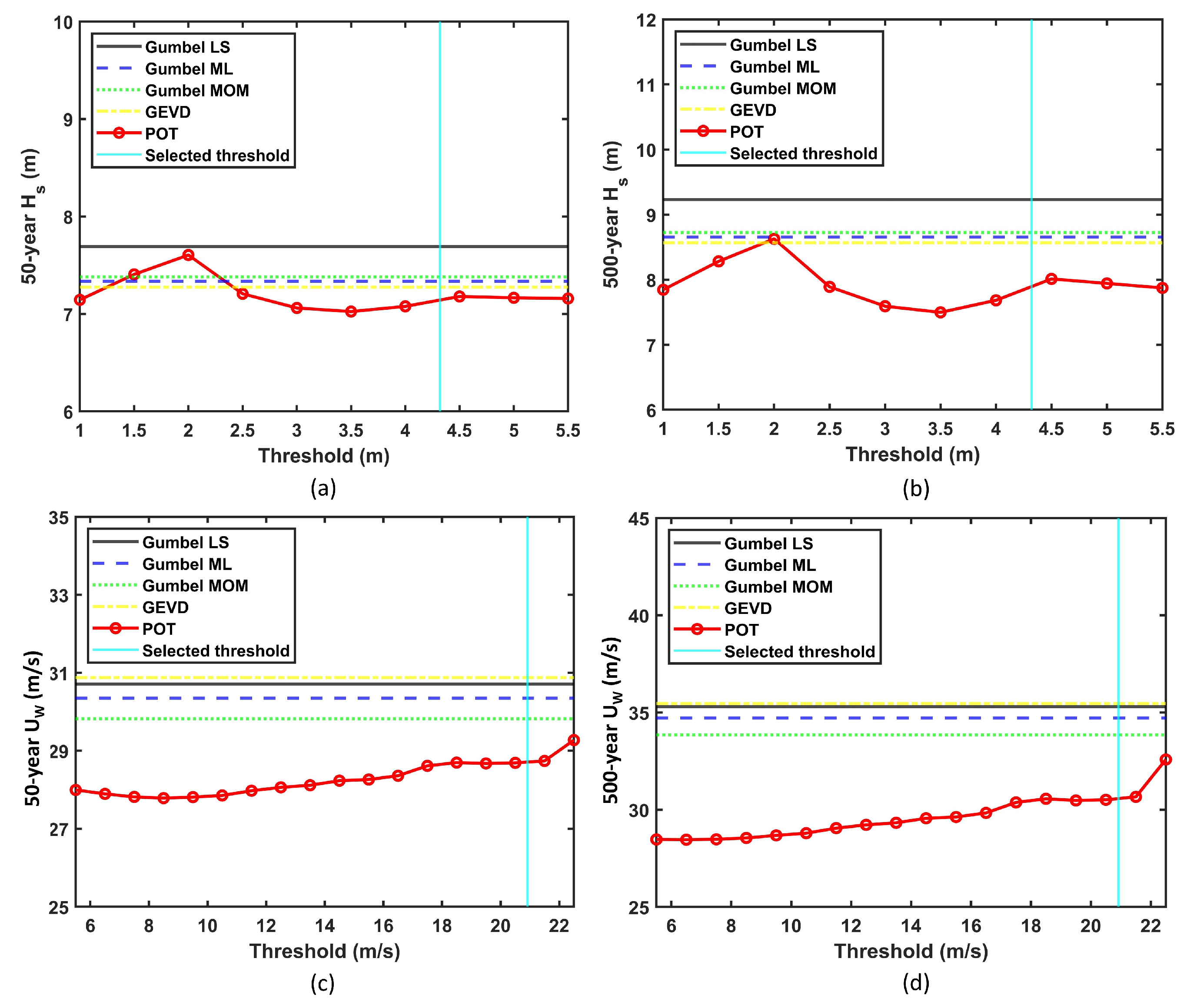
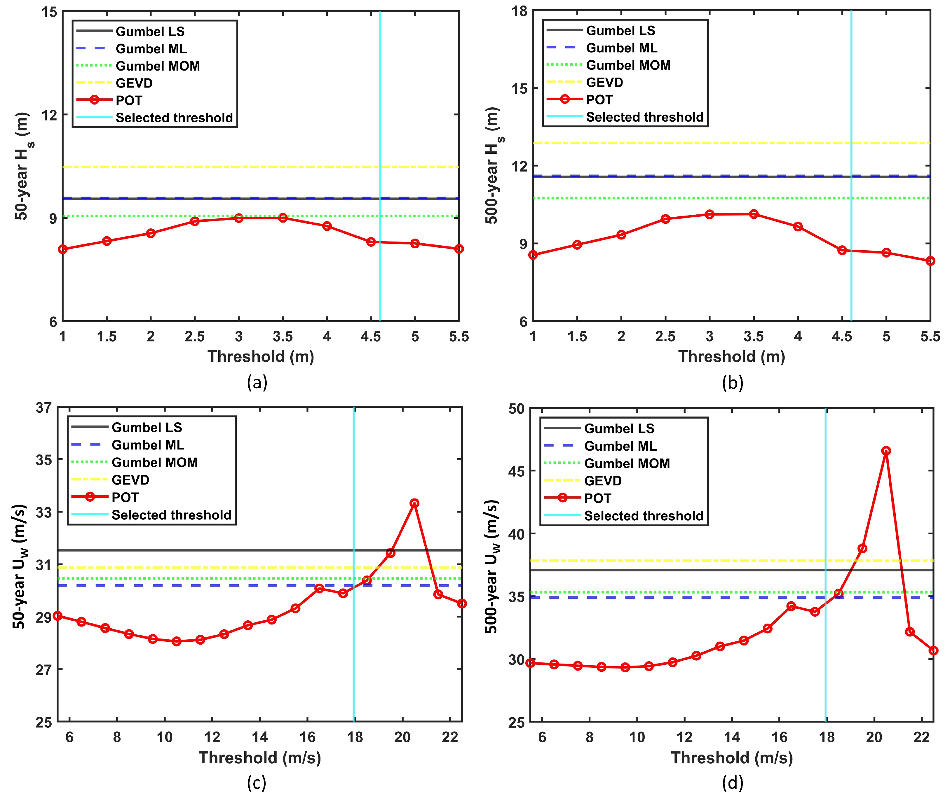
- The results from the POT approach varied significantly based on the chosen threshold.
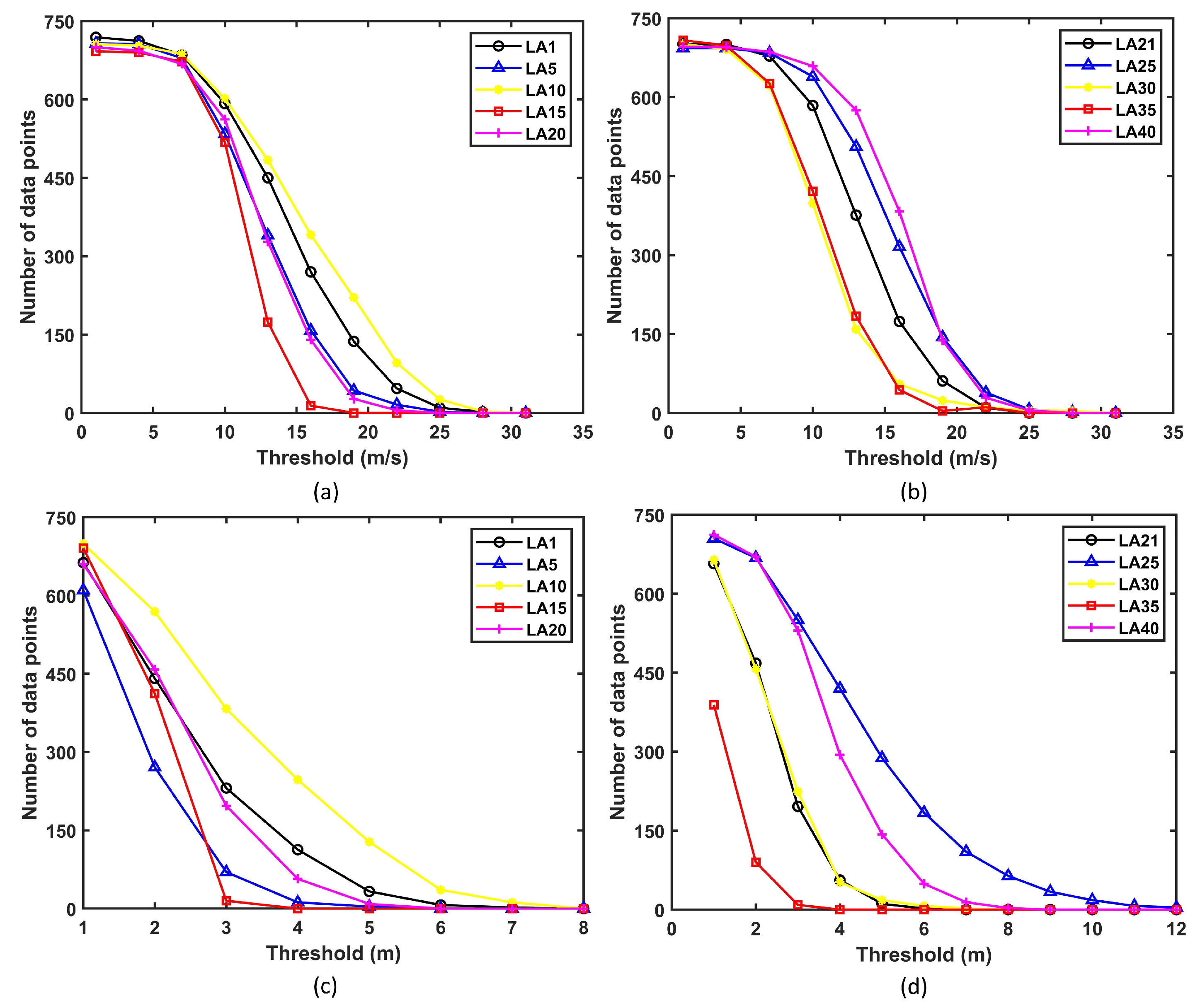
- For smaller thresholds, the results from the POT approach were sensitive to the time window chosen. However, the time window did not have an impact on the results for larger thresholds, which were generally obtained from the mean residual life method.
- The POT approach is only effective for a small range of thresholds. Smaller thresholds lead to a poor fit to the GPD, while larger thresholds may not provide sufficient data points.
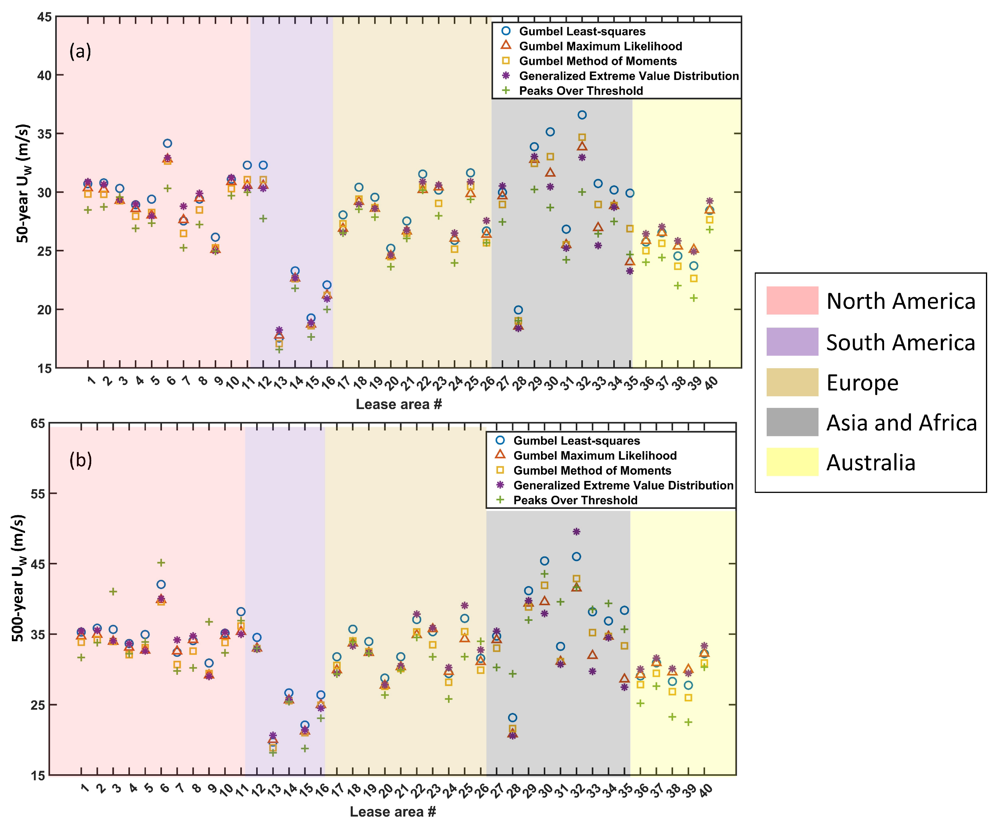
- The 50-year at 10 m above the sea level ranged between 16.5 m/s and 36.5 m/s. The 500-year ranged from 18.1 m/s to 49.5 m/s.
- The 50-year lay between 2.8 m and 15.1 m. The 500-year varied from 3.2 m to 18.7 m.
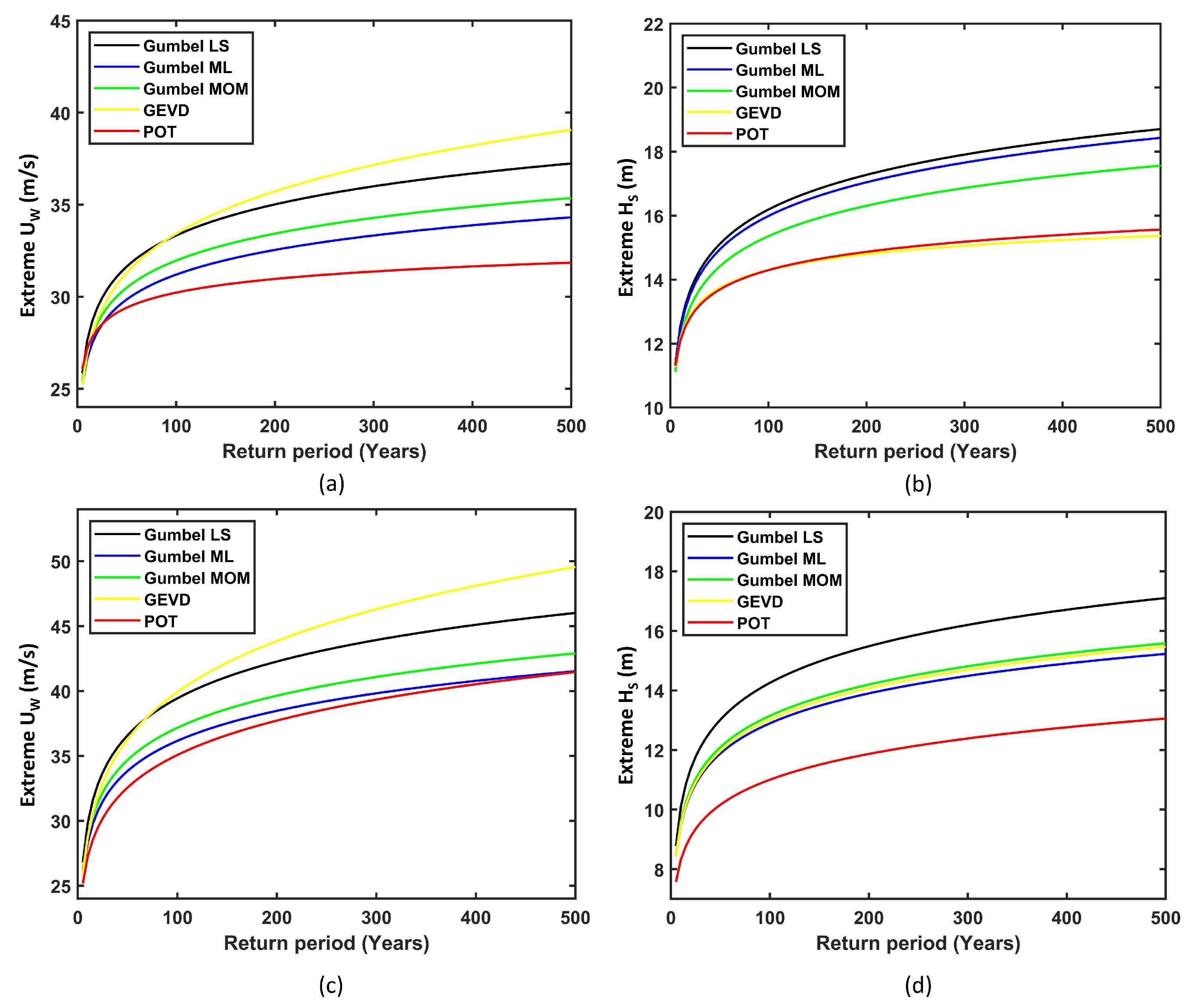
- It is found that the block-maxima approach using the Gumbel LS and GEV distributions provides upper bound estimates for the 50- and 500-year extreme values for both the and .
- The estimates from the POT approach were generally lower by around 3% on average, although there were some outliers.
- European sites are more prone to extreme values in general. LA25 (GoliatVIND, Norway) produced the highest 50- and 500-year values of 15.1 m (Gumbel LS) and 18.7 m (Gumbel LS), respectively.
- Sites along the east coast of China have high estimates of extreme values. LA32 (Minyang Jieyang Qianzhan III, China) was prone to the highest 50- and 500-year values of 36.5 m/s (Gumbel LS) and 49.5 m/s (GEVD), respectively.
- The distribution parameters were provided for all of the methods, which would be helpful for extrapolating the extreme values to longer return periods.
- The mean residual life method used for estimating the optimal threshold has yielded results that lie close to or within the bounds of the estimates from the block-maxima approach.
Future Work
Author Contributions
Funding
Data Availability Statement
Acknowledgments
Conflicts of Interest
References
- GWEC. Global Wind Report. 2023. Available online: https://gwec.net/wp-content/uploads/2023/04/GWEC-2023_interactive.pdf (accessed on 22 July 2023).
- Barthelmie, R.J.; Dantuono, K.E.; Renner, E.J.; Letson, F.L.; Pryor, S.C. Extreme wind and waves in US east coast offshore wind energy lease areas. Energies 2021, 14, 1053. [Google Scholar] [CrossRef]
- IRENA. World Energy Transitions Outlook 2023: 1.5 °C Pathway. 2023. Available online: https://mc-cd8320d4-36a1-40ac-83cc-3389-cdn-endpoint.azureedge.net/-/media/Files/IRENA/Agency/Publication/2023/Jun/IRENA_World_energy_transitions_outlook_v1_2023.pdf?rev=261b3ae18f70429ea8cf595d5a4bee18 (accessed on 22 July 2023).
- Putuhena, H.; White, D.; Gourvenec, S.; Sturt, F. Finding space for offshore wind to support net zero: A methodology to assess spatial constraints and future scenarios, illustrated by a UK case study. Renew. Sustain. Energy Rev. 2023, 182, 113358. [Google Scholar] [CrossRef]
- Zhao, Z.; Li, X.; Wang, W.; Shi, W. Analysis of dynamic characteristics of an ultra-large semi-submersible floating wind turbine. J. Mar. Sci. Eng. 2019, 7, 169. [Google Scholar]
- Hopewell, P.; Castro-Sayas, F.; Bailey, D. Optimising the design of offshore wind farm collection networks. In Proceedings of the IEEE 41st International Universities Power Engineering Conference, Newcastle Upon Tyne, UK, 6–8 September 2006; Volume 1, pp. 84–88. [Google Scholar]
- IEC 61400-3-1:2019; Wind Turbines Part 3-1: Design Requirements for Fixed OffshoreWind Turbines. Edition 1.0 2019-04, IEC FDIS: Geneva, Switzerland, 2019; p. 314.
- Pryor, S.C.; Barthelmie, R.J. A global assessment of extreme wind speeds for wind energy applications. Nat. Energy 2021, 6, 268–276. [Google Scholar]
- Izaguirre, C.; Méndez, F.J.; Menéndez, M.; Losada, I.J. Global extreme wave height variability based on satellite data. Geophys. Res. Lett. 2011, 38. [Google Scholar] [CrossRef]
- Lee, B.H.; Ahn, D.J.; Kim, H.G.; Ha, Y.C. An estimation of the extreme wind speed using the Korea wind map. Renew. Energy 2012, 42, 4–10. [Google Scholar] [CrossRef]
- Sacré, C. Extreme wind speed in France: The’99 storms and their consequences. J. Wind. Eng. Ind. Aerodyn. 2002, 90, 1163–1171. [Google Scholar] [CrossRef]
- Torrielli, A.; Repetto, M.P.; Solari, G. The annual rate of independent events for the analysis of the extreme wind speed. J. Wind. Eng. Ind. Aerodyn. 2016, 156, 104–114. [Google Scholar] [CrossRef]
- Palutikof, J.P.; Brabson, B.; Lister, D.H.; Adcock, S. A review of methods to calculate extreme wind speeds. Meteorol. Appl. 1999, 6, 119–132. [Google Scholar]
- Wang, J.; Qin, S.; Jin, S.; Wu, J. Estimation methods review and analysis of offshore extreme wind speeds and wind energy resources. Renew. Sustain. Energy Rev. 2015, 42, 26–42. [Google Scholar]
- Hong, H.; Li, S.; Mara, T. Performance of the generalized least-squares method for the Gumbel distribution and its application to annual maximum wind speeds. J. Wind. Eng. Ind. Aerodyn. 2013, 119, 121–132. [Google Scholar] [CrossRef]
- Lombardo, F.T. Improved extreme wind speed estimation for wind engineering applications. J. Wind. Eng. Ind. Aerodyn. 2012, 104, 278–284. [Google Scholar] [CrossRef]
- Afzal, M.S.; Kumar, L.; Chugh, V.; Kumar, Y.; Zuhair, M. Prediction of significant wave height using machine learning and its application to extreme wave analysis. J. Earth Syst. Sci. 2023, 132, 51. [Google Scholar] [CrossRef]
- Simiu, E.; Heckert, N.A. Extreme wind distribution tails: A “peaks over threshold” approach. J. Struct. Eng. 1996, 122, 539–547. [Google Scholar] [CrossRef]
- Viselli, A.M.; Forristall, G.Z.; Pearce, B.R.; Dagher, H.J. Estimation of extreme wave and wind design parameters for offshore wind turbines in the Gulf of Maine using a POT method. Ocean. Eng. 2015, 104, 649–658. [Google Scholar] [CrossRef]
- An, Y.; Pandey, M. A comparison of methods of extreme wind speed estimation. J. Wind. Eng. Ind. Aerodyn. 2005, 93, 535–545. [Google Scholar] [CrossRef]
- Kang, D.; Ko, K.; Huh, J. Determination of extreme wind values using the Gumbel distribution. Energy 2015, 86, 51–58. [Google Scholar] [CrossRef]
- Rivas, D.; Caleyo, F.; Valor, A.; Hallen, J. Extreme value analysis applied to pitting corrosion experiments in low carbon steel: Comparison of block maxima and peak over threshold approaches. Corros. Sci. 2008, 50, 3193–3204. [Google Scholar] [CrossRef]
- Vinoth, J.; Young, I. Global estimates of extreme wind speed and wave height. J. Clim. 2011, 24, 1647–1665. [Google Scholar] [CrossRef]
- Jonathan, P.; Ewans, K. Uncertainties in extreme wave height estimates for hurricane-dominated regions. J. Offshore Mech. Arct. Eng. 2007, 129, 300–305. [Google Scholar] [CrossRef]
- Pandey, M.D.; Van Gelder, P.; Vrijling, J. The estimation of extreme quantiles of wind velocity using L-moments in the peaks-over-threshold approach. Struct. Saf. 2001, 23, 179–192. [Google Scholar] [CrossRef]
- Karpa, O.; Naess, A. Extreme value statistics of wind speed data by the ACER method. J. Wind. Eng. Ind. Aerodyn. 2013, 112, 1–10. [Google Scholar] [CrossRef]
- Gaidai, O.; Xing, Y.; Balakrishna, R.; Xu, J. Improving extreme offshore wind speed prediction by using deconvolution. Heliyon 2023, 9, e13533. [Google Scholar] [CrossRef] [PubMed]
- 4COffshore. Offshore Wind Energy Map. 2023. Available online: https://map.4coffshore.com/offshorewind/ (accessed on 21 June 2023).
- NCEI. The Multibeam Bathymetry Database (MBBDB). 2023. Available online: https://www.ncei.noaa.gov/maps/bathymetry/ (accessed on 21 June 2023).
- WaveClimate Infoplaza. Available online: http://www.waveclimate.com/ (accessed on 20 June 2023).
- Peter Groenewoud, S.H. Validation of the BMTA 35-Year Hindcast Database v361, Technical Report, BMT ARGOSS: Houten, The Netherlands, 2016. Available online: http://www.waveclimate.com/clams/redesign/help/docs/I113_Validation_BMTA_35-year_Hindcast_17jun2016.pdf (accessed on 21 June 2023).
- Bali, T.G. The generalized extreme value distribution. Econ. Lett. 2003, 79, 423–427. [Google Scholar] [CrossRef]
- Cooray, K. Generalized gumbel distribution. J. Appl. Stat. 2010, 37, 171–179. [Google Scholar] [CrossRef]
- Brodtkorb, P.A.; Johannesson, P.; Lindgren, G.; Rychlik, I.; Rydén, J.; Sjö, E. WAFO-a Matlab toolbox for analysis of random waves and loads. In Proceedings of the ISOPE International Ocean and Polar Engineering Conference (ISOPE 2000), Seattle, WA, USA, 27 May–2 June 2000. [Google Scholar]
- Mahdi, S.; Cenac, M. Estimating Parameters of Gumbel Distribution using the Methods of Moments, probability weighted Moments and maximum likelihood. Rev. Mat. Teor. Apl. 2005, 12, 151–156. [Google Scholar] [CrossRef]
- Gibson, R.; Grant, C.; Forristall, G.Z.; Smyth, R.; Owrid, P.; Hagen, O.; Leggett, I. Bias and uncertainty in the estimation of extreme wave heights and crests. In Proceedings of the International Conference on Offshore Mechanics and Arctic Engineering, Honolulu, HI, USA, 31 May–6 June 2009; Volume 43420, pp. 363–373. [Google Scholar]
- Castillo, E.; Hadi, A.S. Fitting the generalized Pareto distribution to data. J. Am. Stat. Assoc. 1997, 92, 1609–1620. [Google Scholar] [CrossRef]
- Greenwood, P.E.; Nikulin, M.S. A Guide to Chi-Squared Testing; John Wiley & Sons: Hoboken, NJ, USA, 1996; Volume 280. [Google Scholar]
- D’Agostino, R. Goodness-of-Fit-Techniques; Routledge: Oxford, UK, 2017. [Google Scholar]
- Anderson, T.W.; Darling, D.A. A test of goodness of fit. J. Am. Stat. Assoc. 1954, 49, 765–769. [Google Scholar] [CrossRef]
- Chu, J.; Dickin, O.; Nadarajah, S. A review of goodness of fit tests for Pareto distributions. J. Comput. Appl. Math. 2019, 361, 13–41. [Google Scholar] [CrossRef]
- NOAA. Tropical Cyclone Climatology. 2023. Available online: https://www.nhc.noaa.gov/climo/ (accessed on 6 July 2023).
- Colbert, A. A Force of Nature: Hurricanes in a Changing Climate. 2022. Available online: https://climate.nasa.gov/news/3184/a-force-of-nature-hurricanes-in-a-changing-climate/ (accessed on 20 July 2023).
- Breivik, Ø.; Aarnes, O.J.; Abdalla, S.; Bidlot, J.R.; Janssen, P.A. Wind and wave extremes over the world oceans from very large ensembles. Geophys. Res. Lett. 2014, 41, 5122–5131. [Google Scholar] [CrossRef]


| Lease Area # | Name | Country | GPS Coordinates | Water Depth (m) |
|---|---|---|---|---|
| 1 | Maine research array | USA | 4323 N, 6921 W | ≈175 |
| 2 | Revolution wind | USA | 418 N,714 W | ≈35 |
| 3 | Ocean wind | USA | 396 N, 7417 W | ≈37.5 |
| 4 | Garden State offshore energy | USA | 3840 N, 7442 W | ≈20 |
| 5 | Empire wind | USA | 4017 N, 7319 W | 21.9–41.14 |
| 6 | OCS-A 0545 | USA | 3327 N, 7758 W | ≈26 |
| 7 | CVOW Commercial Project | USA | 3654 N, 7520 W | 21.9–38.1 |
| 8 | Cascadia wind | USA | 4646 N, 12439 W | ≈150 |
| 9 | Morro Bay E | USA | 3531 N, 12141 W | ≈150 |
| 10 | Allan array | Canada | 5137 N, 12843 W | ≈35 |
| 11 | Sea-Breeze Tech | Canada | 462 N, 6149 W | ≈50 |
| 12 | UY01 | Uruguay | 3414 S, 5140 W | ≈50 |
| 13 | Projeto Acu | Brazil | 228 S, 4044 W | ≈50 |
| 14 | Farol wind | Brazil | 2851 S, 4841 W | ≈50 |
| 15 | Sopros do RJ | Brazil | 2137 S, 4025 W | ≈27 |
| 16 | Projeto Ubu | Brazil | 2051 S, 4023 W | ≈27 |
| 17 | Voyage | Ireland | 5121 N, 721 W | ≈85 |
| 18 | Inch Cape | United Kingdom | 5629 N, 211 W | ≈25 |
| 19 | Nordlicht I | Germany | 5417 N, 613 E | ≈35 |
| 20 | Baltic offshore alpha | Sweden | 5817 N, 1821 E | ≈36 |
| 21 | Bornholm bassin syd | Denmark | 5450 N, 1534 E | ≈57 |
| 22 | Vigso bay | Denmark | 5710 N, 839 E | ≈14 |
| 23 | Calabria | Italy | 3826 N, 1652 E | ≈475 |
| 24 | Normandie | France | 4952 N, 049 W | ≈45 |
| 25 | GoliatVIND | Norway | 7149 N, 2234 E | 300–400 |
| 26 | Nao Victoria | Spain | 3617 N, 443 W | ≈300 |
| 27 | Genesis Hexicon | South Africa | 302 S, 3138 E | ≈500 |
| 28 | E3 | India | 750 N, 7749 E | ≈50 |
| 29 | Miaoli | Taiwan | 2439 N, 12038 E | ≈50 |
| 30 | Huaneng Hainan Wenchang 1 | China | 1958 N, 1113 E | ≈120 |
| 31 | Huaneng Daishan I | China | 3018 N, 12142 E | ≈10 |
| 32 | Minyang Jieyang Qianzhan III | China | 2238 N, 11627 E | ≈40 |
| 33 | Boryeong | South Korea | 3614 N, 1264 E | ≈6 |
| 34 | Satsuma | Japan | 3149 N, 1308 E | ≈40 |
| 35 | Southern Mindoro | Philippines | 1152 N, 12128 E | ≈26 |
| 36 | Leeuwin | Australia | 331 S, 11517 E | ≈40 |
| 37 | Mid West | Australia | 2932 S, 11435 E | ≈50 |
| 38 | Southern winds | Australia | 389 S, 14047 E | ≈35 |
| 39 | Barwon | Australia | 3844 S, 14218 E | ≈78 |
| 40 | South Taranaki | New Zealand | 3932 S, 17340 E | ≈36 |
| Lease Area # | Gumbel LS | Gumbel ML | Gumbel MOM | GEVD | POT | ||||||
|---|---|---|---|---|---|---|---|---|---|---|---|
| k | k | ||||||||||
| 1 | 22.97 | 1.98 | 22.98 | 1.89 | 23.03 | 1.74 | −0.16 | 1.98 | 23.14 | 0.21 | 3.31 |
| 2 | 22.24 | 2.19 | 22.27 | 2.04 | 22.31 | 1.92 | −0.11 | 2.12 | 22.39 | 0.15 | 3.13 |
| 3 | 21.26 | 2.32 | 21.34 | 2.03 | 21.34 | 2.03 | −0.02 | 2.04 | 21.36 | 0.05 | 2.73 |
| 4 | 20.90 | 2.06 | 20.93 | 1.96 | 20.97 | 1.79 | −0.15 | 2.02 | 21.08 | 0.13 | 2.81 |
| 5 | 20.01 | 2.40 | 20.12 | 2.02 | 20.10 | 2.09 | 0.02 | 2.01 | 20.10 | 0.12 | 2.90 |
| 6 | 20.82 | 3.42 | 20.87 | 3.06 | 20.92 | 3.00 | −0.02 | 3.08 | 20.90 | 0.02 | 2.70 |
| 7 | 19.28 | 2.11 | 19.28 | 2.14 | 19.37 | 1.82 | −0.36 | 2.33 | 19.69 | 0.16 | 2.99 |
| 8 | 21.49 | 2.03 | 21.50 | 2.05 | 21.56 | 1.78 | −0.19 | 2.10 | 21.71 | 0.23 | 3.62 |
| 9 | 18.12 | 2.06 | 18.19 | 1.77 | 18.19 | 1.81 | 0.03 | 1.74 | 18.16 | 0.001 | 1.73 |
| 10 | 24.28 | 1.75 | 24.30 | 1.69 | 24.34 | 1.52 | −0.14 | 0.65 | 24.43 | 0.22 | 3.11 |
| 11 | 22.34 | 2.55 | 22.48 | 2.07 | 22.43 | 2.21 | 0.06 | 2.02 | 22.42 | 0.12 | 3.12 |
| 12 | 21.16 | 2.15 | 21.20 | 1.90 | 21.23 | 1.89 | 0.020 | 1.88 | 21.18 | 0.14 | 2.94 |
| 13 | 13.97 | 0.92 | 13.96 | 0.98 | 14.01 | 0.78 | −0.41 | 1.04 | 14.18 | 0.17 | 1.15 |
| 14 | 17.55 | 1.47 | 17.60 | 1.29 | 17.60 | 1.28 | −0.02 | 1.30 | 17.61 | 0.12 | 1.62 |
| 15 | 14.46 | 1.23 | 14.49 | 1.08 | 14.52 | 1.05 | −0.05 | 1.11 | 14.52 | 0.24 | 1.50 |
| 16 | 14.83 | 1.86 | 14.86 | 1.63 | 14.89 | 1.61 | 0.08 | 1.56 | 14.79 | 0.14 | 1.68 |
| 17 | 21.74 | 1.62 | 21.81 | 1.30 | 21.79 | 1.41 | 0.12 | 1.24 | 21.73 | 0.20 | 2.70 |
| 18 | 21.48 | 2.29 | 21.55 | 1.96 | 21.55 | 2.01 | 0.06 | 1.90 | 21.49 | 0.15 | 3.20 |
| 19 | 22.13 | 1.90 | 22.21 | 1.63 | 22.20 | 1.66 | −0.005 | 1.64 | 22.22 | 0.16 | 2.90 |
| 20 | 19.18 | 1.54 | 19.23 | 1.37 | 19.24 | 1.35 | −0.03 | 1.38 | 19.25 | 0.20 | 2.62 |
| 21 | 20.33 | 1.84 | 20.43 | 1.59 | 20.42 | 1.56 | −0.04 | 1.61 | 20.47 | 0.17 | 2.90 |
| 22 | 22.18 | 2.40 | 22.25 | 2.03 | 22.25 | 2.10 | 0.08 | 1.97 | 22.17 | 0.09 | 2.76 |
| 23 | 21.42 | 2.24 | 21.46 | 2.30 | 21.51 | 1.93 | −0.16 | 2.29 | 21.66 | 0.20 | 3.89 |
| 24 | 19.93 | 1.52 | 19.92 | 1.57 | 19.99 | 1.32 | −0.26 | 1.63 | 20.15 | 0.25 | 2.67 |
| 25 | 22.20 | 2.42 | 22.33 | 1.93 | 22.28 | 2.10 | 0.12 | 1.83 | 22.20 | 0.14 | 2.92 |
| 26 | 18.46 | 2.10 | 18.46 | 2.03 | 18.54 | 1.83 | −0.29 | 2.25 | 18.78 | 0.07 | 2.49 |
| 27 | 21.98 | 2.05 | 21.98 | 1.97 | 22.06 | 1.76 | −0.23 | 2.12 | 22.24 | 0.19 | 2.45 |
| 28 | 14.54 | 1.38 | 14.70 | 0.98 | 14.64 | 1.12 | 0.08 | 0.95 | 14.66 | −0.06 | 0.84 |
| 29 | 21.54 | 3.16 | 21.61 | 2.86 | 21.64 | 2.77 | −0.05 | 2.91 | 21.69 | 0.11 | 2.87 |
| 30 | 17.83 | 4.44 | 18.10 | 3.46 | 17.99 | 3.85 | 0.15 | 3.23 | 17.83 | 0.03 | 3.04 |
| 31 | 15.98 | 2.78 | 16.03 | 2.43 | 16.08 | 2.42 | 0.05 | 2.37 | 15.97 | −0.01 | 1.95 |
| 32 | 20.68 | 4.08 | 20.87 | 3.32 | 20.82 | 3.55 | 0.12 | 3.15 | 20.66 | 0.02 | 2.57 |
| 33 | 18.17 | 3.22 | 18.51 | 2.16 | 18.33 | 2.72 | 0.28 | 1.86 | 18.20 | 0.02 | 2.08 |
| 34 | 18.89 | 2.89 | 18.95 | 2.53 | 18.99 | 2.53 | 0.02 | 2.51 | 18.92 | 0.04 | 2.65 |
| 35 | 15.62 | 3.66 | 16.33 | 1.97 | 15.97 | 2.80 | 0.16 | 1.82 | 16.15 | 0.03 | 2.16 |
| 36 | 20.13 | 1.44 | 20.12 | 1.47 | 20.19 | 1.23 | −0.30 | 1.56 | 20.36 | 0.33 | 3.38 |
| 37 | 19.11 | 1.90 | 19.11 | 1.90 | 19.18 | 1.65 | −0.20 | 1.98 | 19.32 | 0.16 | 2.09 |
| 38 | 18.25 | 1.62 | 18.23 | 1.83 | 18.33 | 1.37 | −0.44 | 1.84 | 18.64 | 0.28 | 2.42 |
| 39 | 16.89 | 1.75 | 16.87 | 2.11 | 17.00 | 1.45 | −0.40 | 1.95 | 17.30 | 0.25 | 2.36 |
| 40 | 22.04 | 1.64 | 22.03 | 1.64 | 22.10 | 1.42 | −0.30 | 1.78 | 22.31 | 0.16 | 2.36 |
| Lease Area # | Gumbel LS | Gumbel ML | Gumbel MOM | GEVD | POT | ||||||
|---|---|---|---|---|---|---|---|---|---|---|---|
| k | k | ||||||||||
| 1 | 5.09 | 0.67 | 5.11 | 0.57 | 5.11 | 0.58 | 0.05 | 0.56 | 5.10 | 0.13 | 1.22 |
| 2 | 5.76 | 1.22 | 5.84 | 0.94 | 5.81 | 1.05 | 0.11 | 0.90 | 5.79 | 0.09 | 1.19 |
| 3 | 3.68 | 0.58 | 3.68 | 0.54 | 3.70 | 0.51 | −0.12 | 0.56 | 3.72 | 0.08 | 0.74 |
| 4 | 5.43 | 1.01 | 5.44 | 1.01 | 5.47 | 0.87 | −0.22 | 1.05 | 5.56 | 0.07 | 1.13 |
| 5 | 3.39 | 0.79 | 3.45 | 0.58 | 3.43 | 0.68 | 0.16 | 0.54 | 3.41 | 0.05 | 0.71 |
| 6 | 4.96 | 1.10 | 4.99 | 0.91 | 5.00 | 0.94 | 0.20 | 0.82 | 4.90 | 0.02 | 0.89 |
| 7 | 3.98 | 0.79 | 4.04 | 0.63 | 4.02 | 0.67 | 0.09 | 0.63 | 4.04 | 0.07 | 0.80 |
| 8 | 7.18 | 0.78 | 7.17 | 0.83 | 7.20 | 0.67 | −0.24 | 0.83 | 7.28 | 0.22 | 1.48 |
| 9 | 4.74 | 0.92 | 4.75 | 0.85 | 4.79 | 0.78 | −0.36 | 1.00 | 4.93 | 0.03 | 0.83 |
| 10 | 6.35 | 0.69 | 6.37 | 0.64 | 6.38 | 0.60 | −0.08 | 0.65 | 6.40 | 0.18 | 1.21 |
| 11 | 4.45 | 0.73 | 4.46 | 0.73 | 4.48 | 0.64 | −0.17 | 0.75 | 4.52 | 0.10 | 0.88 |
| 12 | 6.80 | 0.71 | 6.83 | 0.57 | 6.82 | 0.62 | 0.08 | 0.56 | 6.81 | 0.15 | 1.21 |
| 13 | 3.68 | 0.40 | 3.68 | 0.38 | 3.69 | 0.35 | −0.14 | 0.40 | 3.71 | 0.11 | 0.47 |
| 14 | 5.10 | 0.59 | 5.12 | 0.51 | 5.12 | 0.52 | 0.02 | 0.51 | 5.11 | 0.13 | 0.79 |
| 15 | 2.84 | 0.26 | 2.85 | 0.24 | 2.85 | 0.23 | −0.05 | 0.24 | 2.85 | 0.13 | 0.30 |
| 16 | 2.16 | 0.22 | 2.17 | 0.18 | 2.17 | 0.19 | 0.09 | 0.17 | 2.16 | 0.15 | 0.27 |
| 17 | 7.56 | 1.06 | 7.60 | 0.93 | 7.60 | 0.91 | −0.04 | 0.94 | 7.62 | 0.17 | 1.71 |
| 18 | 5.43 | 1.03 | 5.42 | 1.04 | 5.47 | 0.88 | −0.36 | 1.13 | 5.63 | 0.06 | 1.13 |
| 19 | 6.40 | 0.71 | 6.41 | 0.64 | 6.42 | 0.62 | −0.07 | 0.66 | 6.43 | 0.23 | 1.33 |
| 20 | 4.49 | 0.53 | 4.50 | 0.44 | 4.50 | 0.46 | 0.07 | 0.43 | 4.49 | 0.15 | 0.88 |
| 21 | 4.40 | 0.67 | 4.43 | 0.55 | 4.42 | 0.58 | 0.05 | 0.54 | 4.42 | 0.12 | 0.87 |
| 22 | 6.15 | 0.87 | 6.15 | 0.88 | 6.20 | 0.73 | −0.59 | 1.04 | 6.43 | 0.13 | 1.31 |
| 23 | 4.69 | 0.80 | 4.69 | 0.82 | 4.73 | 0.68 | −0.32 | 0.87 | 4.84 | 0.09 | 1.00 |
| 24 | 4.32 | 0.56 | 4.33 | 0.53 | 4.34 | 0.48 | −0.15 | 0.55 | 4.38 | 0.20 | 0.90 |
| 25 | 9.02 | 1.56 | 9.03 | 1.51 | 9.07 | 1.37 | −0.16 | 1.58 | 9.16 | 0.10 | 1.82 |
| 26 | 4.00 | 0.67 | 4.00 | 0.64 | 4.03 | 0.58 | −0.23 | 0.69 | 4.09 | 0.10 | 0.90 |
| 27 | 7.49 | 0.93 | 7.51 | 0.84 | 7.52 | 0.80 | −0.07 | 0.86 | 7.54 | 0.18 | 1.41 |
| 28 | 2.60 | 0.47 | 2.66 | 0.29 | 2.63 | 0.38 | 0.14 | 0.27 | 2.64 | 0.06 | 0.36 |
| 29 | 4.01 | 0.84 | 4.05 | 0.71 | 4.05 | 0.72 | −0.003 | 0.72 | 4.05 | 0.09 | 0.72 |
| 30 | 4.49 | 1.01 | 4.52 | 0.87 | 4.53 | 0.89 | 0.11 | 0.83 | 4.47 | −0.001 | 0.70 |
| 31 | 2.08 | 0.45 | 2.09 | 0.41 | 2.10 | 0.39 | −0.09 | 0.42 | 2.11 | 0.01 | 0.32 |
| 32 | 6.14 | 1.77 | 6.25 | 1.44 | 6.21 | 1.51 | 0.01 | 1.44 | 6.24 | −0.04 | 0.86 |
| 33 | 3.19 | 0.59 | 3.24 | 0.42 | 3.21 | 0.51 | 0.24 | 0.37 | 3.19 | 0.07 | 0.55 |
| 34 | 4.00 | 0.82 | 4.02 | 0.75 | 4.03 | 0.71 | −0.09 | 0.77 | 4.06 | 0.06 | 0.79 |
| 35 | 2.40 | 0.58 | 2.46 | 0.42 | 2.43 | 0.49 | 0.15 | 0.39 | 2.42 | 0.07 | 0.55 |
| 36 | 4.70 | 0.61 | 4.69 | 0.67 | 4.73 | 0.52 | −0.35 | 0.68 | 4.82 | 0.22 | 1.05 |
| 37 | 6.73 | 0.69 | 6.74 | 0.65 | 6.75 | 0.60 | −0.12 | 0.67 | 6.78 | 0.14 | 1.12 |
| 38 | 7.52 | 0.80 | 7.51 | 0.84 | 7.56 | 0.68 | −0.31 | 0.88 | 7.66 | 0.20 | 1.34 |
| 39 | 5.28 | 0.54 | 5.28 | 0.52 | 5.30 | 0.47 | −0.17 | 0.54 | 5.33 | 0.19 | 0.86 |
| 40 | 6.54 | 0.72 | 6.55 | 0.69 | 6.57 | 0.63 | −0.14 | 0.71 | 6.60 | 0.17 | 1.19 |
Disclaimer/Publisher’s Note: The statements, opinions and data contained in all publications are solely those of the individual author(s) and contributor(s) and not of MDPI and/or the editor(s). MDPI and/or the editor(s) disclaim responsibility for any injury to people or property resulting from any ideas, methods, instructions or products referred to in the content. |
© 2023 by the authors. Licensee MDPI, Basel, Switzerland. This article is an open access article distributed under the terms and conditions of the Creative Commons Attribution (CC BY) license (https://creativecommons.org/licenses/by/4.0/).
Share and Cite
Bhaskaran, S.; Verma, A.S.; Goupee, A.J.; Bhattacharya, S.; Nejad, A.R.; Shi, W. Comparison of Extreme Wind and Waves Using Different Statistical Methods in 40 Offshore Wind Energy Lease Areas Worldwide. Energies 2023, 16, 6935. https://doi.org/10.3390/en16196935
Bhaskaran S, Verma AS, Goupee AJ, Bhattacharya S, Nejad AR, Shi W. Comparison of Extreme Wind and Waves Using Different Statistical Methods in 40 Offshore Wind Energy Lease Areas Worldwide. Energies. 2023; 16(19):6935. https://doi.org/10.3390/en16196935
Chicago/Turabian StyleBhaskaran, Saravanan, Amrit Shankar Verma, Andrew J. Goupee, Subhamoy Bhattacharya, Amir R. Nejad, and Wei Shi. 2023. "Comparison of Extreme Wind and Waves Using Different Statistical Methods in 40 Offshore Wind Energy Lease Areas Worldwide" Energies 16, no. 19: 6935. https://doi.org/10.3390/en16196935
APA StyleBhaskaran, S., Verma, A. S., Goupee, A. J., Bhattacharya, S., Nejad, A. R., & Shi, W. (2023). Comparison of Extreme Wind and Waves Using Different Statistical Methods in 40 Offshore Wind Energy Lease Areas Worldwide. Energies, 16(19), 6935. https://doi.org/10.3390/en16196935