Future Cities Carbon Emission Models: Hybrid Vehicle Emission Modelling for Low-Emission Zones

Abstract

Current emission models primarily focus on traditional combustion vehicles and may not accurately represent emissions from the increasingly diverse vehicle fleet. The growing presence of hybrid and electric vehicles requires the development of accurate emission models to measure the emissions and energy consumption of these vehicles. This issue is particularly relevant for low-emission zones within cities, where effective mobility planning relies on simulation models using continuously updated databases. This research presents a two-dimensional emission model for hybrid vehicles, employing artificial neural networks for low-emission zones. The key outcome is the methodology developed to create a CO₂ emission model tailored for hybrid vehicles, which can be used to simulate various road solutions. The CO₂ emission model achieved an R² coefficient of 0.73 and an MSE of 0.91, offering valuable information for further advancements in emission modelling.

1. Introduction

Cities around the world are pursuing sustainable development goals, particularly in the context of sustainable mobility. Urban mobility is becoming a key aspect of urban transformation [1]. The concepts of the cities of the future involve not only the development of new technologies and innovations but also the revision of traditional approaches to urban planning and traffic management [2]. The aim of the cities of the future is to create an urban environment that is people-friendly, energy-efficient, and at the same time reduces negative environmental impacts [3,4]. Sustainable mobility includes reducing vehicle emissions by reducing congestion, improving accessibility to public transport, and developing alternative forms of mobility, such as electric scooters, bicycles, and car sharing [5,6].

One way to deal with the problem of increased emissions in cities is by creating so-called low-emission zones [7]. These zones are areas within a city where vehicle emission standards are regulated. The purpose of these zones is to reduce the impact of urban transport on air quality and to promote cleaner transport technologies [8]. By reducing vehicle emissions, greenhouse gas emissions are also reduced to a large extent. This is important in the context of climate change. Zones encourage the use of vehicles with lower emissions, such as hybrid or electric vehicles, which reduces CO₂ emissions [9]. The implementation of low-emission zones is a complex process that requires appropriate infrastructure, vehicle emissions, regulation, and the education of drivers and residents. As cities strive to create more friendly and sustainable urban environments, low-emission zones are an important instrument to achieve these goals by controlling emissions promoting cleaner transportation solutions. An example of a low-emission zone is the City of London, where the city has introduced the ‘London Ultra Low emission Zone’, which covers the inner city and aims to significantly reduce vehicle emissions [10]. The introduction of this zone has contributed to a significant improvement in air quality in London. Another example is the city of Berlin, which has introduced the ‘Umweltzone’, which covers a large area of the city [11]. These introduce requirements for vehicle emission standards, meaning that only vehicles that meet certain standards are allowed to enter certain areas of the city [12].

By meeting these goals and evaluating them, it is possible to influence the quality of life of residents. Properly designed and managed transport systems reduce queueing times, improve accessibility to jobs and services, and significantly reduce negative impacts on public health. Reducing greenhouse gas emissions, especially carbon dioxide, also helps combat climate change.

One of the main challenges for the cities of the future is to reduce harmful emissions and promote the more efficient use of energy in road transport. Most current emission models mainly focus on combustion vehicles [13]. These models are not adequately equipped to represent diverse vehicle ecosystem, which includes an increasing share of hybrid and electric vehicles. By way of example, the model [14] describes its road emissions for internal combustion vehicles operating on petrol, diesel, and LPG (liquefied petroleum gas). The model has an increased level of detail because it is based on local data, while it does not take into account alternative propulsion systems such as hybrids at all. Another example is the work [15]. The study focusses on adapting the US-EPA’s MOVES emissions model for use in Hyderabad, India, by addressing the disparities in driving conditions and vehicle-specific factors. The default model, based on US driving cycles, is not representative of India’s unique driving conditions. To rectify this, the researchers incorporated a modified Indian driving cycle and a local driving cycle for light-duty vehicles, resulting in revised emission rates.

Most of the work addresses the problem of creating emission models, but does not consider the creation of new models for new types of vehicles [16,17]. As a result, there is the gap and a need to develop more accurate emission models that take into account the diversity of vehicles (hybrid propulsion) in low-emission urban zones.

In the context of the development of new emission models, it is necessary to use them skilfully for traffic simulation purposes. For the planning of new solutions or the modification of existing solutions in cities, the simulation of vehicle and pedestrian traffic is carried out to forecast traffic flow and safety for future investments. As an example, the work [18] presents the problem of autonomous vehicle traffic simulation in the context of emission generation. This work concerns the analysis of different types of autonomous vehicles and their driving style on NO_x, CO₂, and PM₁₀ emissions. The simulations in this work were performed in Vissim. Another example of Vissim use in vehicle emission analyses is [19]. This work concerns analyses of balanced permissiveness solutions at an X junction, for which different methods of giving way to priority for crossing were used. The results show practical recommendations for the applicability of specific traffic signs for the analysis of NOx and PM₁₀ emissions.

Taking into account the information provided above and the reviewed work, this work focusses on the creation of a new CO₂ emission model for a hybrid vehicle dedicated to low-emission urban zones, which can be used in combination with traffic microsimulation tools. The emission model was created using real data from the portable emission measurement system (PEMS) and is based on an artificial neural network method. The model was validated with a coefficient of determination of R² (coefficient of determination) of 0.73 and a mean square error (MSE)of 0.91. In the next stage of the study, the model was used in a simulation analysis of three selected urban traffic solutions for low-emission zones: speed limits at pedestrian crossings, raised crossing zones, and a scenario with traffic slowing in the form of speed bumps on the roadway. The results of CO₂ emission obtained from the simulations studied can serve as initial recommendations for the design of such road solutions.

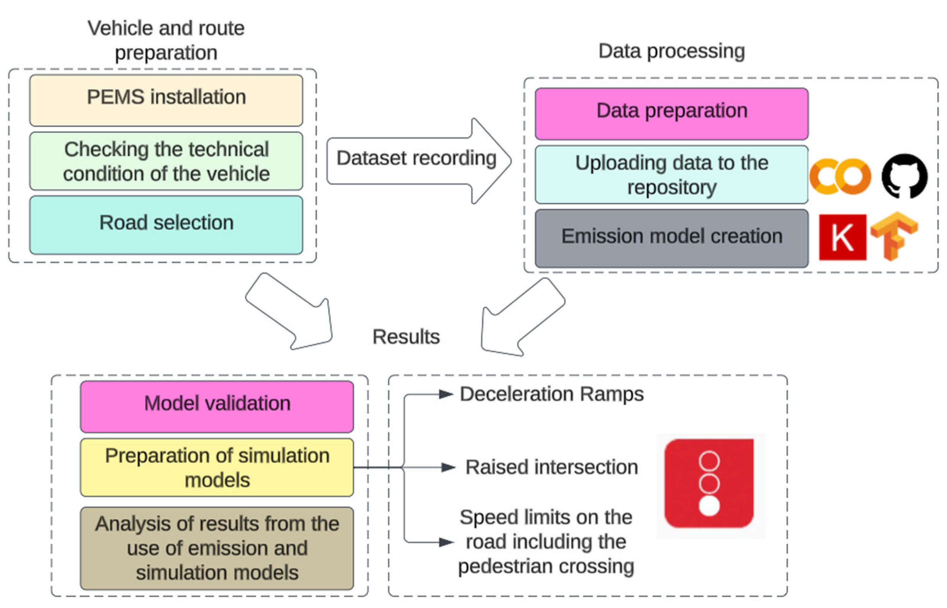
2. Materials and Methods

The general scheme of this work is shown in Figure 1. In the first stage of the work, the prepared vehicle was prepared for test runs with the installed portable emission measurement system (PEMS). The PEMS system was mounted on the rear seat of the vehicle and in its boot. Furthermore, the vehicle was checked for technical performance at a vehicle inspection station before road tests were carried out. An important part of the work was also the preparation of a defined route. The basic requirement for the route was to drive through different parts of the city to collect as much data as possible, which is needed for the CO₂ emission model for the hybrid vehicle. The challenge here is additionally that, for some parts of the journey. the combustion engine is turned off, and for some traffic conditions, it is switched on. In the next stage of the work, the data were processed and placed in a data repository. For this purpose, a free Github file repository can be used, or the Google Colab data repository. A CO₂ model was then created using the Tensorflow/Keras libraries, which are available for the Python programming language. The model was validated using the R² coefficient of determination and MSE. Then, 3 moments of potential solutions that are used in current cities and will be used in future cities were made in Vissim software (ver. 2023). Scenarios were modelled for speed bumps, raised intersections, and speed limits at pedestrian crossings. For these simulation scenarios, the developed CO₂ emissions model was used to map the emissions generated by vehicles. In relation to the results obtained, the paper proposes recommendations for the applicability of these solutions in future cities.

The PEMS system was used to collect CO₂ emissions and vehicle movement data. The vehicle selected for this study is shown in Figure 2. The selected technical parameters of the vehicle are presented in

Table 1. Selected technical parameters of research vehicle.

Year of manufacture	2020
Engine type	Hybrid
Engine capacity	1497 cm3
Internal combustion engine: power	67 kW
Internal combustion engine: maximum torque	111 Nm 3600–4400 RPM
Ignition	Spark
Electric motor type	Permanent magnet electric motor
Electric motor: power	59 kW
Electric motor: maximum torque	169 Nm
Exhaust after-treatment system	Three-way catalytic converter (TWC)
Exhaust emissions standard	Euro 6d
Traction battery	Nickel-hydride
Fuel tank capacity	36 L
Unladen mass	min. 1085/max. 1095 kg

.

The investigated driving route is presented as a CO₂ map in Figure 3. The route was 55 km long, the average speed on this route was 55 km/h, while 3600 data records were generated on it with a recording frequency of 1 Hz.

The CO₂ emissions data collected from the hybrid vehicle for the tested is summarised in a 3D chart in relation to the velocity and acceleration parameter (Figure 4).

2.1. Data Collection and Processing

The data collected from PEMS were converted into .xls format and then transferred to the Google Collaboration file repository. Google Colaboratory, often referred to as Colab, is a free cloud-based platform for working with Jupyter notebooks offered by Google [20]. Colab allows access to popular libraries and tools for machine learning and data analysis, such as TensorFlow, PyTorch, or Pandas, without the need to install and configure a local programming environment [21,22]. The data were split into a learning set and a testing set in an 80/20 ratio, and a neural network technique from the Tensorflow library was used to create the emission model along with the integrated Keras. TensorFlow is an open source machine learning platform developed by Google. It is one of the most popular tools for building and training machine learning models and neural networks. Keras is an open source deep learning framework that serves as an interface for the popular TensorFlow library. It provides a user-friendly and high-level API for designing and training neural networks, making it accessible for both beginners and experts in machine learning. Two variables—V (velocity) and a (acceleration)—were used to perform the CO₂ prediction model. By using only two explanatory variables, the model created will be more accessible, e.g., for its use with traffic simulation data.

The algorithm used to create the neural network model is as follows (Algorithm 1).

Algorithm 1. CO2 emission model for a hybrid vehicle, source code.

import pandas as pd

import numpy as np

from sklearn.model_selection import train_test_split

from sklearn.preprocessing import StandardScaler

import tensorflow as tf

from tensorflow import keras

from tensorflow.keras import layers

from sklearn.metrics import mean_squared_error

# Load data from the data repository

file_path = “/content/hybrid po filtracji.xlsx”  # Update this with the actual file path

df = pd.read_excel(file_path)

# Select features (V and a) and target variable (CO2)

X = df[[‘V’, ‘a’]].values

y = df[‘CO2 g/s’].values

# Split the data into training and testing sets

X_train, X_test, y_train, y_test = train_test_split(X, y, test_size = 0.2, random_state = 42)

# Standardize the features

scaler = StandardScaler()

X_train_scaled = scaler.fit_transform(X_train)

X_test_scaled = scaler.transform(X_test)

# Build the neural network model

model = keras.Sequential([

layers.Input(shape = (2,)),  # Input layer with 2 features (V and a)

layers.Dense(64, activation = ‘relu’),  # Hidden layer with 64 neurons and ReLU activation

layers.Dense(1)  # Output layer with 1 neuron for CO2 prediction

])

# Compile the model

model.compile(optimizer = ‘adam’, loss = ‘mean_squared_error’)

# Train the model

model.fit(X_train_scaled, y_train, epochs = 50, batch_size = 32, validation_split = 0.2, verbose = 1)

# Evaluate the model

y_pred = model.predict(X_test_scaled)

mse = mean_squared_error(y_test, y_pred)

print(f”Mean Squared Error: {mse:.2f}”)

From the above neural network model algorithm, we can see which libraries were used in Google Colab. The neural network model was built using the TensorFlow/Keras library. The model contains three layers: an input layer with two features (V and a), a hidden layer with 64 neurons, a ReLU activation function, and an output layer with one neurone (CO₂ prediction). The model is compiled using the loss function ‘mean_squared_error’ (mean squared error) and the optimiser ‘adam’. This loss is used as a metric to evaluate the model error. The model is trained on the training data using the fit function. Training is performed for 50 epochs with a batch size of 32. The model is also dated on a portion of the training data. After training, the model is evaluated on the test data. The mean square error (MSE) result is displayed on the console to assess the accuracy of the model in predicting the target variables from the new data.

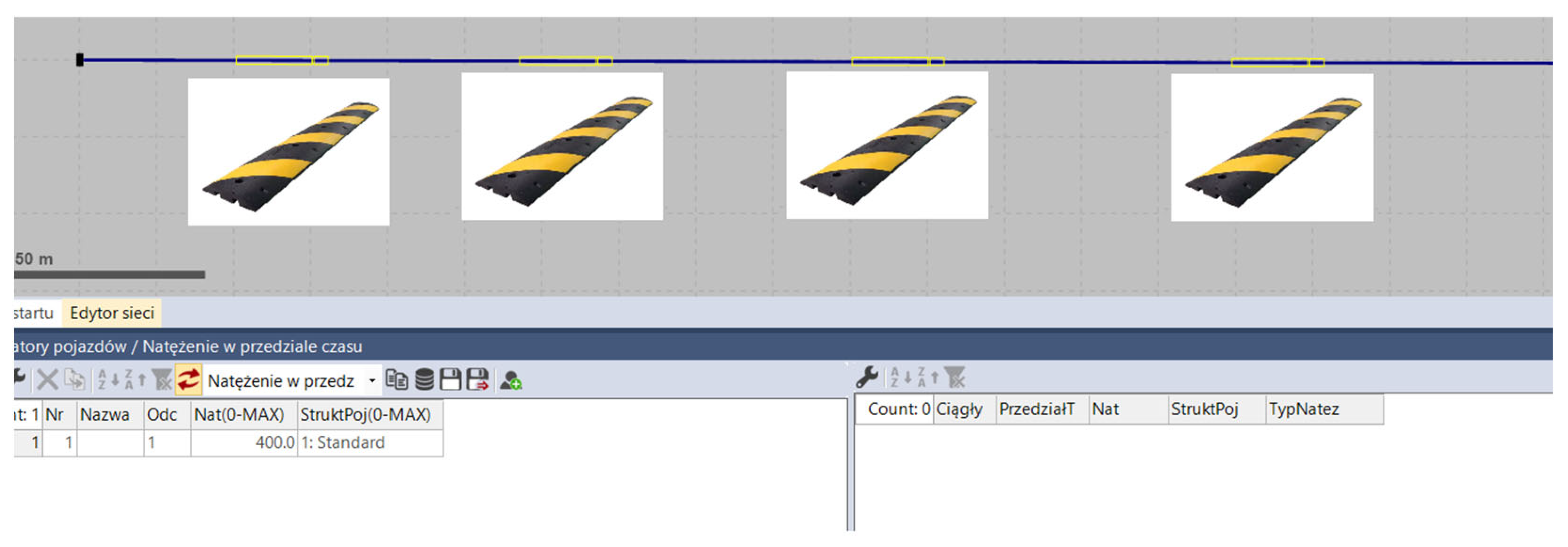
2.2. Analysed Scenarios

For the data collected and the CO₂ emission model performed, an additional analysis of its potential use was carried out in this study. Vissim software was used for this purpose. Vissim is a traffic modelling tool for future cities. It is a comprehensive traffic simulation software tool to analyse, plan, and optimise transport systems in urban environments [23,24]. In the cities of the future, where sustainable mobility and efficient traffic management are a priority, Vissim plays a key role. It allows the creation of advanced traffic models that take into account different types of vehicles, road infrastructure, traffic lights, driver and passenger behaviour, making it possible to simulate the introduction of innovative solutions such as autonomous vehicles and car sharing [25,26]. Vissim assumes three scenarios for the use of a CO₂ emission model for a hybrid vehicle for exemplary road solutions for low-emission zones in cities:

• Speed bumps for 4 different deceleration speeds—30 km/h, 25 km/h, 20 km/h, and 15 km/h.
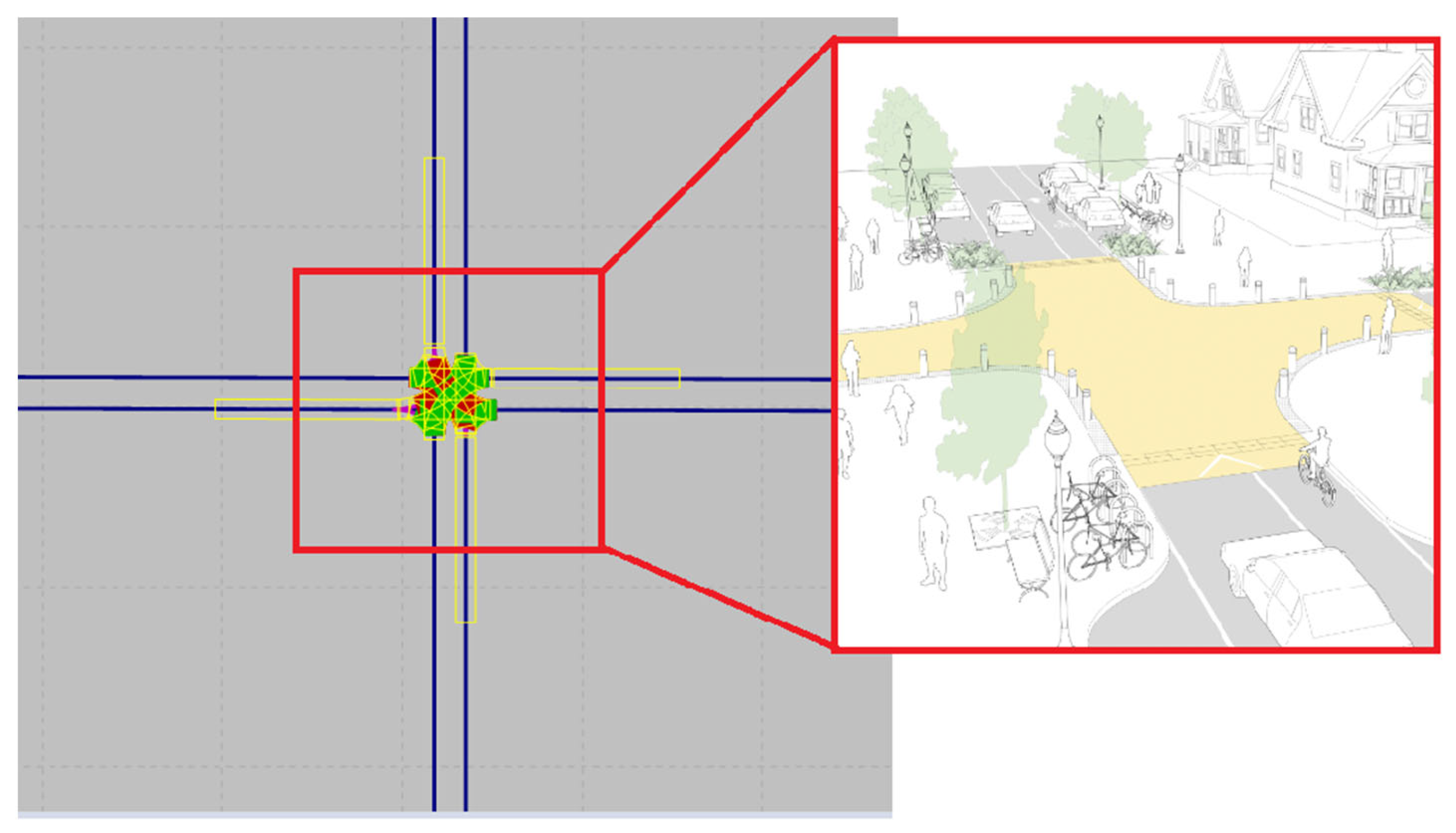
• Raised X-shaped intersection.
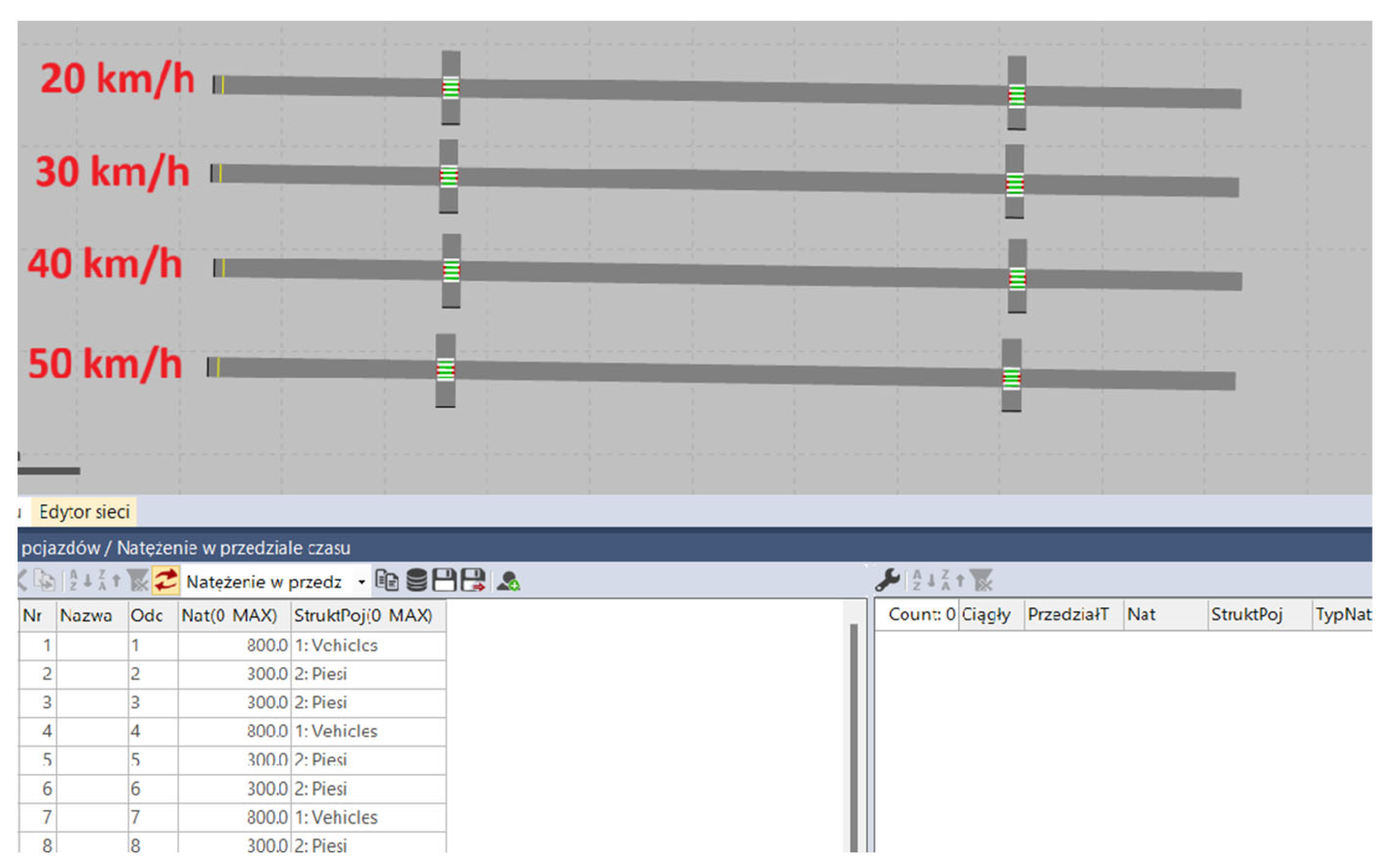
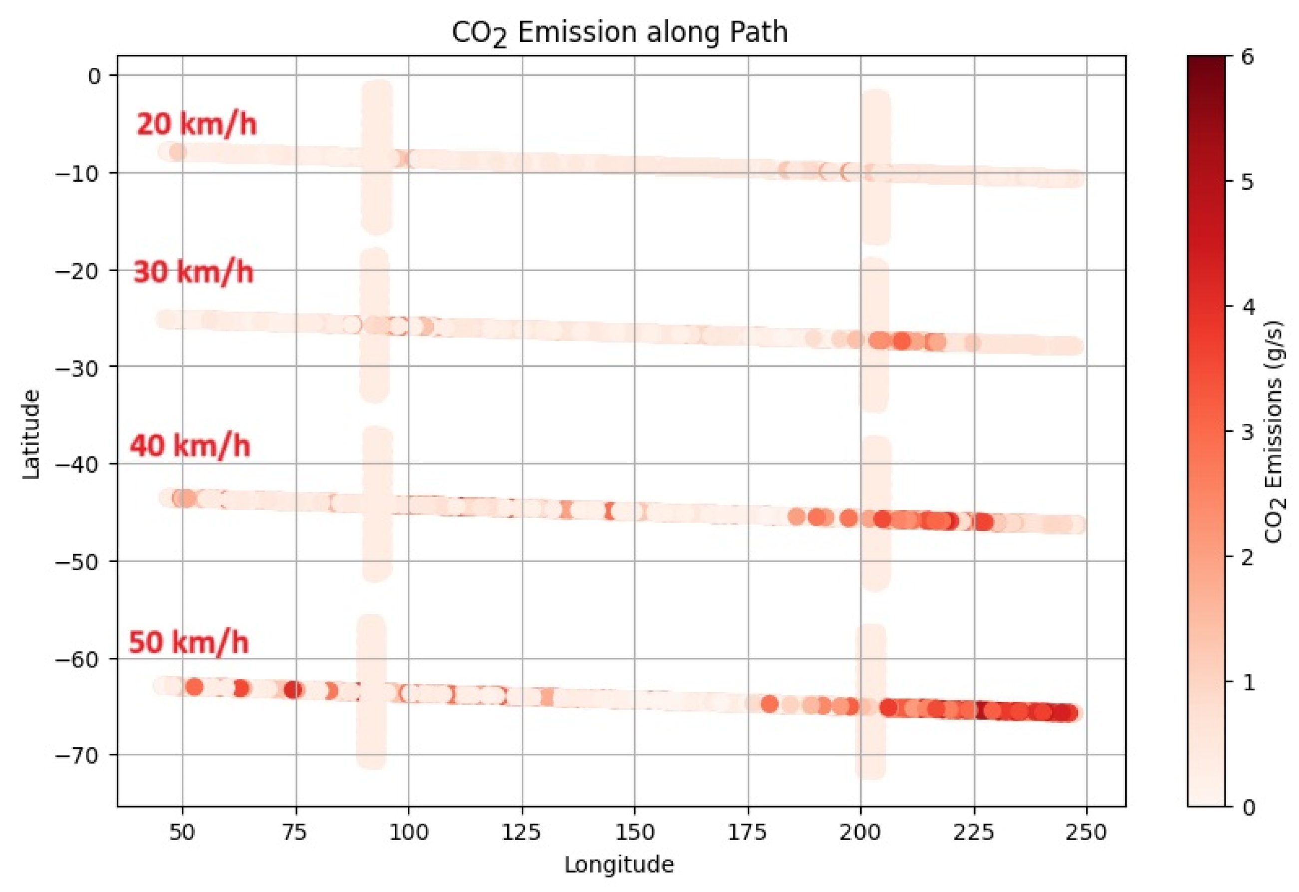
• Road speed limits including pedestrian crossing, tested speeds: 20 km/h, 30 km/h, 40 km/h, 50 km/h.

For the described scenarios, models were prepared in Vissim, for which simulations lasting 3600 s were carried out in order to aggregate the traffic data for further processing of the prepared CO₂ emission model. In particular, data were generated from Vissim software for the position of these vehicles and for their speed and acceleration. The data were saved in .fzp format, allowing it to be further processed in any format, such as .xls or .csv.

3. Results

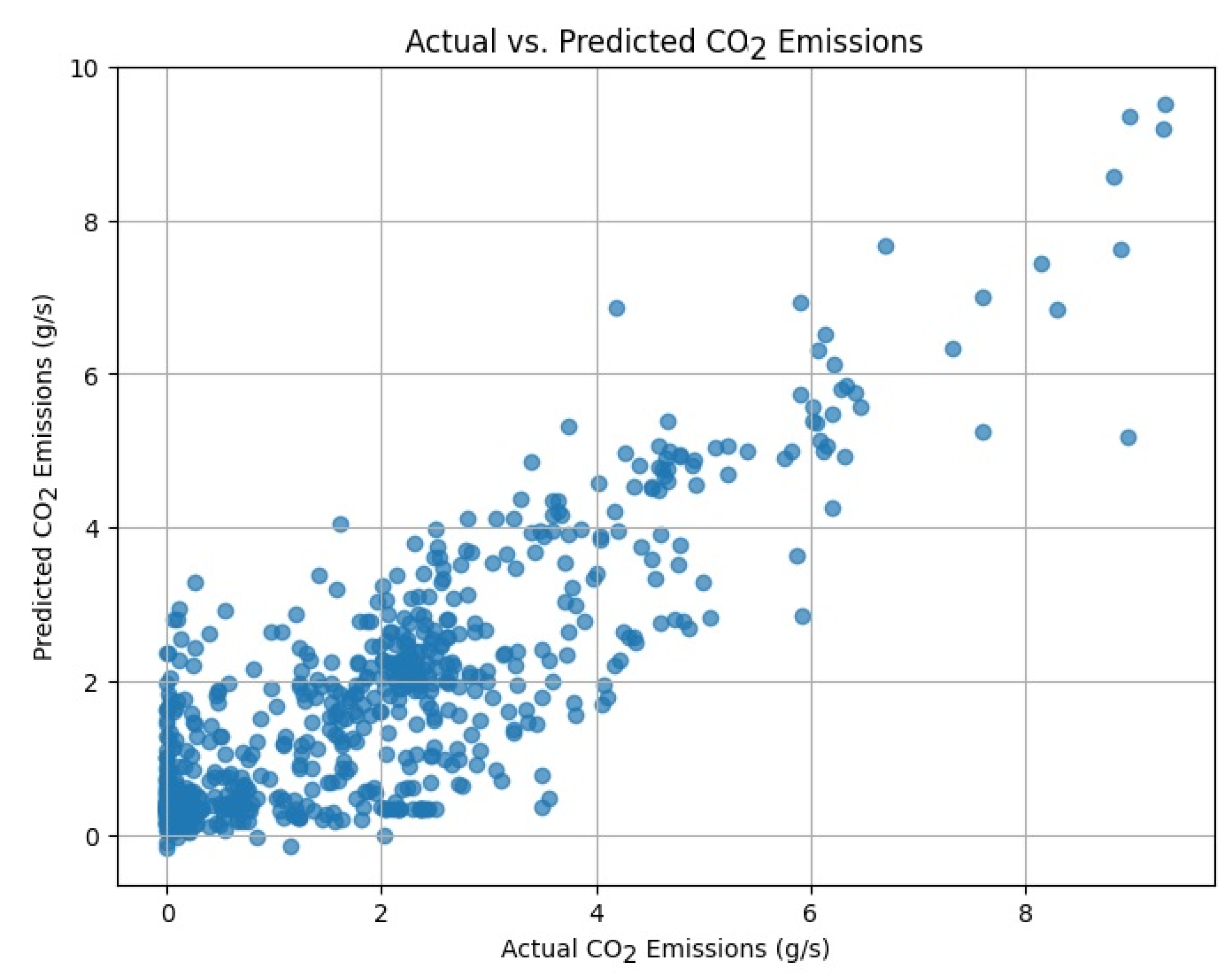
3.1. Emission Model Creation and Validation

The CO₂ emission model was created using the Tensorflow/Keras library, but subsequent validation was important. The validation of a neural network model is a key step in assessing its effectiveness and ability to make accurate predictions. In this context, two important evaluation measures are often used: the R² determination coefficient (R-squared) and the mean square error (MSE).

The evaluation of the artificial neural network models is a key step in the process of developing and improving them. The actual vs. predicted graph plays an important role in this analysis. This allows us to visually compare how well our model predicts the actual data. The main purpose is to see whether the predicted values are close to the actual values, which would indicate the effectiveness of the model [27]. The value of this graph also lies in identifying outlier observations that may be important cases for further analysis. In addition, the graph allows one to assess the linearity of the model’s predictions and identify possible nonlinear patterns in the data. This graph is shown in Figure 5.

The coefficient of determination R² is a measure that tells us to what extent our model is able to explain the variability in the data. The R² value ranges from 0 to 1, where 0 means that the model does not explain the variation in the data and 1 means that the model perfectly predicts the data. The R² value measures how much of the variability in the target variable is explained by the model [28]. The higher the R² value, the better the model performs in terms of prediction.

$$R^2=\frac{S{S}_M}{S{S}_T}=\frac{{\sum }_{t=1}^n\left(\widehat{y}{ }_t-\overline{y}\right){ }^2}{{\sum }_{t=1}^n\left(y_t-\overline{y}\right){ }^2}$$

(1)

where:

• R²—coefficient of determination;
• $S{S}_M$—sum of squares for the model;
• $S{S}_T$—total sum of squares;
• $\widehat{y}{ }_t$—the actual value of the dependent variable;
• $\overline{y}$—predicted values of the dependent variable;
• $y_t$—the average value of the actual dependent variable.

The mean square error (MSE) is a measure that determines how much the predicted values differ from the actual values in the data. Calculate the squared error for each observation and then calculate the average of these errors [29]. The MSE is particularly useful for determining how well a model performs in terms of prediction accuracy, and a lower MSE value indicates a better model.

$$MSE=\frac{\sum (\widehat{y}{ }_t-\overline{y})}{n}$$

(2)

where:

• $\widehat{y}{ }_t$—the actual value of the dependent variable;
• $\overline{y}-$ predicted values of the dependent variable;
• $n$—number of observations.

For the model tested, the R² coefficient is 0.73, while the MSE is 0.91.

Summarising the above techniques for creating an emission model, the next step was to create a simulation model in Vissim software. Simulations in Vissim generated a file that contained velocity and acceleration profiles, and then these profiles served as input to the created emission model using neural networks. The generation of emission data on this basis allowed the creation of emission maps, for which the input data were the CO₂ emission itself and the coordinates of all vehicles.

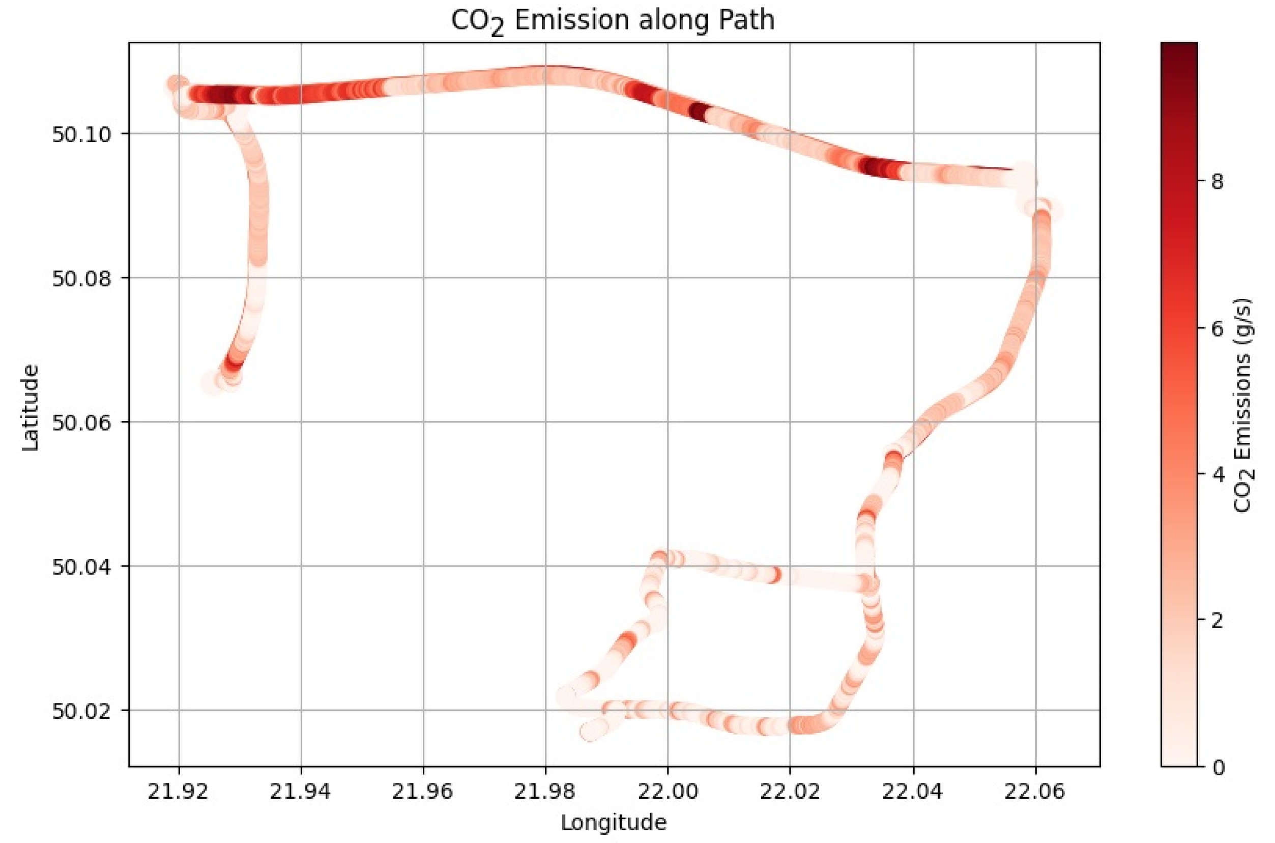
3.2. Simulation Results

3.2.1. Speed Bumps

The simulations were carried out using Vissim software. The first simulation scenario analysed speed bumps for four different deceleration speeds: 30 km/h, 25 km/h, 20 km/h and 15 km/h. Traffic barriers are an important element of creating sustainable mobility in the cities of the future. These physical elements of the road infrastructure aim to reduce the speed of vehicles on certain sections of the road. Their implementation has several important benefits. First, speed bumps increase road safety by reducing the risk of road accidents and possible human injury and loss of life [30,31]. Second, they have an impact on controlling exhaust and noise emissions, which contributes to improving air quality in the city. This statement particularly applies to hybrid vehicles, which are able to run an electric motor at lower speeds and thus minimise emissions. Third, speed bumps introduce elements that slow traffic, which can encourage the use of more environmentally friendly modes of transport, such as cycling and walking [32]. A view of the model is shown in Figure 6, together with an indication of the location of the speed bumps.

The speed bumps were modelled as speed-restricted areas. Speed bumps were placed on a 400 m long road, with a traffic volume of 400 vehicles/h. For the given speed limit zones, a certain area in front of the threshold was set to slow down the vehicle to a given set speed with a deceleration of 3 m/s². The generated data from the.fzp file were imported into the developed CO₂ emissions model into Google Colab. An emissions map was used to develop the CO₂ emission results. A view of the CO₂ emissions map for the route section with thresholds is shown in Figure 7.

From Figure 7, it can be seen:

• Areas of increased vehicle emissions in the vicinity of speed bumps;
• The highest emissions are observed at the threshold where vehicles slow down to the lowest speed of 15 km/h and then proceed to accelerate to the desired speed and fluctuate around 6 g/s of CO₂;
• The smallest CO₂ emissions are for the threshold where vehicles slow down to 30 km/h.

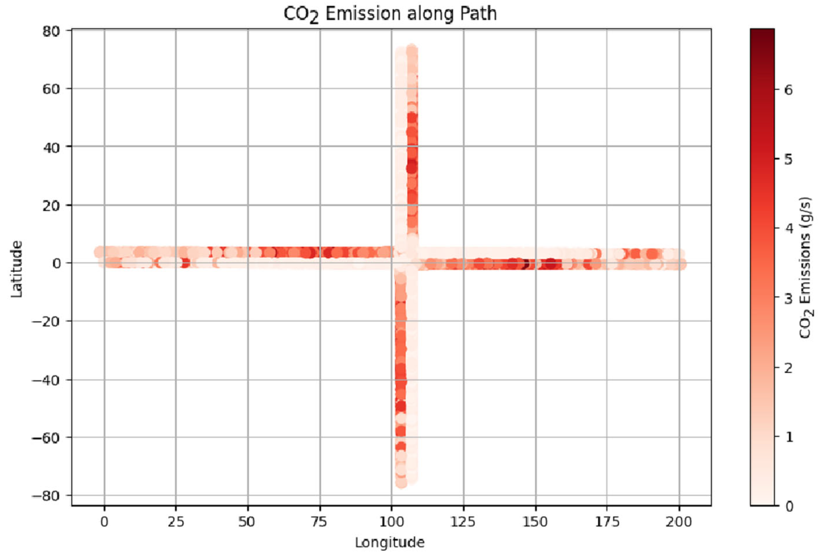
3.2.2. Raised Intersection

The raised intersection is an innovative solution in the context of future urban mobility, which contributes to improving traffic flow and increasing safety at intersections. It is characterised by a raised level of the road surface, creating a kind of platform element that raises the level of the highway to the level of the pavement or the cycle path [33]. This solution allows one to clearly separate the pedestrian and cycling zone from the motor vehicle traffic lane, which increases the safety and comfort of using these means of transport. Furthermore, elevated intersections are often equipped with traffic lights adapted to the needs of pedestrians and cyclists, which promotes sustainable mobility and encourages the use of more environmentally friendly modes of transport [34]. In cities of the future, where the priority is to improve the quality of life of the inhabitants and to reduce traffic congestion and emissions, elevated intersections are a valuable tool in the design of an efficient and person-friendly transport system. A model showing a raised intersection is shown in Figure 8.

The raised intersection was modelled as the usual road sections in Vissim, while speed limit zones were added at the approaches to the intersection and at the intersection itself to simulate vehicle movements and changes in speed. For the 20 m section before the intersection, vehicle speeds were limited to 25 km/h, while at the intersection itself, vehicles travelled at 15 km/h. Additionally, collision fields were set up for simulation so that there were no collision situations between traffic participants. A traffic volume of 400 vehicles/h was established for all roads entering the junction. The results of the hybrid vehicle emissions for the junction under study are shown in Figure 9.

Based on the emission map in Figure 9, it can be observed:

• For the CO₂ model of the hybrid vehicle, low or zero emissions are visible for the approach roads; this is related to approaching the intersection, braking the vehicle, and switching on the electric motor;
• For exit roads, areas of increased CO₂ emissions can be seen, which in places exceed 6 g/s, after driving through the elevated part of the junction;
• Based on the observation of the vehicle emission map, it is possible to look for places where these emissions are lower, making it possible to optimise the placement of pedestrian crossings to minimise the impact of exhaust fumes on the health of pedestrians.

3.2.3. Speed Limits on the Road with Pedestrian Crossings

Vehicle speed limits play a key role in modern mobility in the cities of the future. They have a significant impact on many aspects, including road safety, reduced emissions, improved air quality, and reduced congestion [35]. Lower speeds also improve the quality of life of residents by reducing traffic noise [36]. To analyse the use of the developed hybrid vehicle CO₂ emission model, road models were prepared in Vissim, for which speed limits were established and pedestrian crossings added. The following driving speeds were tested: 20 km/h, 30 km/h, 40 km/h, and 50 km/h. Road models can be seen in Figure 10.

The modelled roads are each 200 m long, but are cut through with pedestrian crossings at two locations. Pedestrians always have priority to enter the carriageway in each case. The volume of vehicle traffic for the roads is 800 vehicles/h, while the volume is 300 pedestrians/h. A visualisation of the CO₂ emissions map as a result of the simulated traffic of vehicles and pedestrians is shown in Figure 11.

Based on the map of the CO₂ emission map in Figure 11 for the studied roads, it can be observed that:

• The lowest CO₂ emissions for the case of a road with a speed limit of 20 km/h is caused by the operation of the vehicle on an electric motor;
• The highest CO₂ emissions for the case of a road with a speed limit of 50 km/h exceed 6 g/s in places;
• In the emission maps, it is possible to see in detail where the highest emissions accumulate, which is caused by the operation of the hybrid drive system, and where increased emissions of other exhaust components can also be observed.

4. Discussion

This paper presents the methodology and process of developing a CO₂ emission model for hybrid vehicles using an artificial neural network technique. In cities of the future, where sustainable mobility and the minimisation of negative environmental impacts are a priority, the development of such models becomes crucial. The discussion of this model aims to highlight its potential applications and implications in the area of road element analysis and the planning of future cities.

Today’s cities face unique challenges related to road traffic and greenhouse gas emissions. CO₂ emission models, based on artificial neural networks, offer a highly accurate and flexible tool that can be adapted to a variety of scenarios and changing conditions. The combination of a CO₂ emission model with traffic simulation tools is also extremely valuable. This makes it possible to assess how different traffic scenarios affect CO₂ emissions from vehicles. This way, city decision-makers and urban planners can accurately analyse the effects of different spatial planning strategies and changes to road infrastructure. This can lead to a more efficient use of resources, less traffic congestion, and, above all, lower emissions of harmful substances and CO₂.

For example, A related work is [37]. The authors propose an efficient methodology to construct a CO₂ emission model. This model creation process, rooted in the evaluation of various methods, including linear and robust regression, fine, medium, and coarse tree models, cubic support vector machines, bagged trees, Gaussian process regression (GPR), and neural networks (NNET), identifies GPR as the most suitable approach for modelling CO₂ emissions based on road input data. Regression learner applications from Matlab were used to create the model. Compared with the method presented in this paper, the use of Google Colab allows emission models to be created and updated much more quickly. The models created there have a lower accuracy than the model presented in this study.

Another study is [38]. This study focusses on modelling the CO₂ emissions of electric vehicles (EVs) and plug-in hybrid electric vehicles (PHEV) in contrast to the CO₂ emissions of conventional internal combustion engine (ICE) vehicles, as reported in the existing literature. PHEVs have the advantage of requiring fewer batteries compared to electric vehicles, making them lighter and potentially more efficient.

There is also work that also exploits the potential of model building in Google Colab in the context of emissions modelling, for example, in [39]. In this work, a CO₂ emissions model is created for a liquefied petroleum gas (LPG) vehicle. The model was developed based on previous exploratory data analysis using gradient machine learning techniques. Vehicle speed and engine speed were chosen as the key explanatory variables to predict CO₂ emissions. The validation process of the model demonstrated its high accuracy, making it a valuable tool for analysing continuous CO₂ emissions and generating emission maps for environmental assessment in an urban context. In particular, for the selected gradient boosting method used to model CO₂ emissions for an LPG vehicle, the validation indices give an R² score of 0.61 and an MSE score of 0.77, confirming the reliability and precision of the model. However, the method described there and the model validation indices indicate an inferior predictive capability of this model compared to the one described in this work.

Another example of work that addresses emissions from hybrid vehicles is [40]. To enhance accuracy, a novel long-short-term memory (LSTM)-based model named UWS-LSTM has been developed, mitigating the shortcomings of existing approaches. The dataset encompasses more than 20 parameters and a rigorous input feature optimisation process has been used to identify the most influential factors. The results underscore the superiority of the UWS-LSTM model, which reaches an impressive 97.5% accuracy compared to traditional ML.

Another article that addresses the complexity of modelling and the impact of carbon emissions on transport is [41]. This paper delves into these methodologies, critically assessing their suitability. Of particular interest is the potential of the micro approach, with an emphasis on information and communication technologies (ICTs), as informed by an extensive review of European projects. The paper’s findings suggest that the micro-approach holds promise, particularly in urban settings, despite the computational complexity and challenges associated with modelling driver behaviour. However, it is acknowledged that addressing numerous sources of scientific uncertainty remains a crucial focus for further research in this domain. Other similar works that need to be taken into account in the context of the complexity of the topic of climate change are those of [42,43].

In order to create more complex models that take into account more factors, e.g., travel elasticity, it is also necessary to take into account how changes in, e.g., travel and policies, affect greenhouse gas emissions. In the context of carbon emissions, travel elasticity plays an essential role in elucidating the intricate dynamics of how alterations in travel patterns and policy interventions can influence greenhouse gas emissions [44,45]. A comprehensive understanding of these elasticities proves indispensable for both policymakers and researchers dedicated to mitigating carbon emissions within the transportation sector [46,47]. By deciphering the nuanced responses of travellers to changes in factors such as pricing, income levels, or travel duration, stakeholders can formulate more nuanced and effective strategies to promote sustainable transportation practises and curtail the carbon footprint associated with travel. For example, the development of efficient public transportation systems, the promotion of carpooling initiatives, and the implementation of congestion pricing mechanisms all exemplify policy approaches that are likely to benefit from a nuanced understanding of travel elasticity [48,49,50]. Such insights become instrumental in the ongoing effort to combat carbon emissions originating from travel, representing a fundamental concern for policymakers and researchers in the realm of environmental sustainability [51].

The emission models created must also be subject to continuous improvement and modification. In discussions of vehicle emissions, a common reference is made to fuel consumption. The scientific literature includes numerous articles that address models to simulate energy consumption and performance in hybrid vehicles, as exemplified in [52] and [53]. Many of these models, developed by various research teams, undergo continuous enhancement and adaptation. For example, [53] was integrated with the modifications presented in [54,55,56].

In conclusion, the development of CO₂ emission models using the methodology presented in this work can provide rapid analysis opportunities that can support municipal authorities’ decision-making in the context of shaping mobility in line with the concept of sustainable mobility in cities of the future. The issues described are particularly relevant in the era of vehicle electrification, causing a very large change in the common vehicle fleet, which is undergoing a metamorphosis and, in some countries, hybrid and electric vehicles are already taking a dominant share [57].

Recommendations

Based on the CO₂ emission model for the hybrid vehicle and the simulation scenarios carried out, the following recommendations can be made to those involved in emissions modelling, vehicle traffic, and decision-makers in municipal authorities.

• A method that gives good results for the prediction of CO₂ emissions for a hybrid vehicle where there are no regular CO₂ emissions associated with the movement of the vehicle due to the switching on of the electric motor and the start-stop system is the artificial neural network method;
• The artificial neural network method gives satisfactory results for the prediction of emissions, given that the input variables for model formation and subsequent prediction of CO₂ are speed V and acceleration a;
• The coefficients R² and MSE for these explanatory variables are high, since taking the Pearson coefficient into account, these variables are approximately 0.6 for velocity V and approximately 0.19 for acceleration;
• These explanatory variables are chosen for the subsequent use of the model in traffic simulations, e.g., in Vissim—which makes the model universally applicable already at the design stage of a road solution;
• Simulations taking into account the different constraints on the speed bumps enable the selection of an appropriate speed-related speed bump design, e.g., the analysis of the selected scenarios shows that the lower the enforced speed of the speed bump, the higher the emissions (of course, the analysis of this for future work should be more extensive and take noise emissions and safety into account);
• For the increased number of hybrid vehicles, increased emissions are to be expected near the raised intersection for outgoing roads, especially near its centre; this gives an idea of the better positioning of pedestrian crossings;
• For the analysis of a speed restriction scenario for roads with pedestrian crossings in future city centres, it can be noted that the introduction of more restrictive speed limits, e.g., 30 km/h, minimises to a large extent the impact of vehicle emissions on the health of pedestrians.

5. Conclusions

This paper presents research in the area of CO₂ modelling for hybrid vehicles, applicable to future cities and their low-emission zones. In this research, an artificial neural network technique was used to create a model of CO₂ emissions from hybrid vehicles. The work points to the growing importance of sustainable mobility and the minimisation of environmental impacts in cities of the future. Adapting emission models to changing traffic conditions and simulating vehicle movements allows accurate analyses of the impact of different urban planning strategies and road infrastructure on CO₂ emissions. The paper also presents existing research work and techniques that are being used in the field of emissions modelling, including technologies such as Google, Colab, and models based on artificial neural networks. This paper points out the benefits of these approaches and presents a novel neural network-based model that achieves high accuracy.

As a result, this article makes a valuable contribution to the development of CO₂ emission models for hybrid vehicles, which can contribute to the creation of more sustainable and greener cities of the future and a better understanding of the environmental impact of mobility.

From the results obtained, it can be observed:

• For the model studied, the R² coefficient is 0.73, while the MSE is 0.91;
• There is a possibility to use the model for the purposes of vehicle traffic analysis with microsimulation tools;
• For the analysed scenarios of speed limits on the road, raised intersections, and speed bumps, we can observe the locations of increased emissions from hybrid vehicles, which allows, for example, the better planning of these solutions in cities.

A limitation of this work is the number of vehicles used in the study, so in the future, it will be necessary to extend the model obtained with new input data. The work also points to the development of a complete hybrid emission estimation software, which will automatically upload the model learning input data and allow one to directly upload input files from simulation tools.

References

1. Belli, L.; Cilfone, A.; Davoli, L.; Ferrari, G.; Adorni, P.; Di Nocera, F.; Dall’Olio, A.; Pellegrini, C.; Mordacci, M.; Bertolotti, E. IoT-Enabled Smart Sustainable Cities: Challenges and Approaches. Smart Cities 2020, 3, 1039–1071. [Google Scholar] [CrossRef]
2. Kharrazi, A.; Qin, H.; Zhang, Y. Urban Big Data and Sustainable Development Goals: Challenges and Opportunities. Sustainability 2016, 8, 1293. [Google Scholar] [CrossRef]
3. Gabaldón Moreno, A.; Vélez, F.; Alpagut, B.; Hernández, P.; Sanz Montalvillo, C. How to Achieve Positive Energy Districts for Sustainable Cities: A Proposed Calculation Methodology. Sustainability 2021, 13, 710. [Google Scholar] [CrossRef]
4. Croese, S.; Green, C.; Morgan, G. Localizing the Sustainable Development Goals Through the Lens of Urban Resilience: Lessons and Learnings from 100 Resilient Cities and Cape Town. Sustainability 2020, 12, 550. [Google Scholar] [CrossRef]
5. Turoń, K.; Kubik, A.; Folęga, P.; Chen, F. Perception of Shared Electric Scooters: A Case Study from Poland. Sustainability 2023, 15, 12596. [Google Scholar] [CrossRef]
6. Jung, J.; Koo, Y. Analyzing the Effects of Car Sharing Services on the Reduction of Greenhouse Gas (GHG) Emissions. Sustainability 2018, 10, 539. [Google Scholar] [CrossRef]
7. Fensterer, V.; Küchenhoff, H.; Maier, V.; Wichmann, H.-E.; Breitner, S.; Peters, A.; Gu, J.; Cyrys, J. Evaluation of the Impact of Low Emission Zone and Heavy Traffic Ban in Munich (Germany) on the Reduction of PM10 in Ambient Air. Int. J. Environ. Res. Public Health 2014, 11, 5094–5112. [Google Scholar] [CrossRef]
8. Lebrusán, I.; Toutouh, J. Using Smart City Tools to Evaluate the Effectiveness of a Low Emissions Zone in Spain: Madrid Central. Smart Cities 2020, 3, 456–478. [Google Scholar] [CrossRef]
9. Cho, S.-H.; Chae, C.-U. A Study on Life Cycle CO2 Emissions of Low-Carbon Building in South Korea. Sustainability 2016, 8, 579. [Google Scholar] [CrossRef]
10. Rizki, M.; Irawan, M.Z.; Dirgahayani, P.; Belgiawan, P.F.; Wihanesta, R. Low Emission Zone (LEZ) Expansion in Jakarta: Acceptability and Restriction Preference. Sustainability 2022, 14, 12334. [Google Scholar] [CrossRef]
11. Morfeld, P.; Stern, R.; Builtjes, P.; Groneberg, D.A.; Spallek, M. Introduction of a low-emission zone and the effect on air pollutant concentration of particulate matter (PM 10)—A pilot study in Munich. Zentralblatt Arbeitsmedizin Arbeitsschutz Ergon. 2013, 63, 104–115. [Google Scholar] [CrossRef]
12. Jiménez-Espada, M.; García, F.M.M.; González-Escobar, R. Citizen Perception and Ex Ante Acceptance of a Low-Emission Zone Implementation in a Medium-Sized Spanish City. Buildings 2023, 13, 249. [Google Scholar] [CrossRef]
13. Mądziel, M. Vehicle Emission Models and Traffic Simulators: A Review. Energies 2023, 16, 3941. [Google Scholar] [CrossRef]
14. Jaworski, A.; Mądziel, M.; Lejda, K. Creating an emission model based on portable emission measurement system for the purpose of a roundabout. Environ. Sci. Pollut. Res. 2019, 26, 21641–21654. [Google Scholar] [CrossRef]
15. Perugu, H. Emission modelling of light-duty vehicles in India using the revamped VSP-based MOVES model: The case study of Hyderabad. Transp. Res. Part D Transp. Environ. 2019, 68, 150–163. [Google Scholar] [CrossRef]
16. Demir, E.; Bektaş, T.; Laporte, G. A comparative analysis of several vehicle emission models for road freight transportation. Transp. Res. Part D Transp. Environ. 2011, 16, 347–357. [Google Scholar] [CrossRef]
17. Smit, R.; Ntziachristos, L.; Boulter, P. Validation of road vehicle and traffic emission models–A review and meta-analysis. Atmos. Environ. 2010, 44, 2943–2953. [Google Scholar] [CrossRef]
18. Beza, A.D.; Maghrour Zefreh, M.; Torok, A. Impacts of Different Types of Automated Vehicles on Traffic Flow Characteristics and Emissions: A Microscopic Traffic Simulation of Different Freeway Segments. Energies 2022, 15, 6669. [Google Scholar] [CrossRef]
19. Mądziel, M.; Campisi, T. Investigation of Vehicular Pollutant Emissions at 4-Arm Intersections for the Improvement of Integrated Actions in the Sustainable Urban Mobility Plans (SUMPs). Sustainability 2023, 15, 1860. [Google Scholar] [CrossRef]
20. Li, Z. Forecasting Weekly Dengue Cases by Integrating Google Earth Engine-Based Risk Predictor Generation and Google Colab-Based Deep Learning Modeling in Fortaleza and the Federal District, Brazil. Int. J. Environ. Res. Public Health 2022, 19, 13555. [Google Scholar] [CrossRef]
21. Ray, S.; Alshouiliy, K.; Agrawal, D.P. Dimensionality Reduction for Human Activity Recognition Using Google Colab. Information 2021, 12, 6. [Google Scholar] [CrossRef]
22. Chang, Y.-H.; Zhang, Y.-Y. Deep Learning for Clothing Style Recognition Using YOLOv5. Micromachines 2022, 13, 1678. [Google Scholar] [CrossRef] [PubMed]
23. Ziemska-Osuch, M.; Osuch, D. Modeling the Assessment of Intersections with Traffic Lights and the Significance Level of the Number of Pedestrians in Microsimulation Models Based on the PTV Vissim Tool. Sustainability 2022, 14, 8945. [Google Scholar] [CrossRef]
24. Chen, C.; Zhao, X.; Liu, H.; Ren, G.; Zhang, Y.; Liu, X. Assessing the Influence of Adverse Weather on Traffic Flow Characteristics Using a Driving Simulator and VISSIM. Sustainability 2019, 11, 830. [Google Scholar] [CrossRef]
25. Mądziel, M.; Jaworski, A.; Savostin-Kosiak, D.; Lejda, K. The Impact of Exhaust Emission from Combustion Engines on the Environment: Modelling of Vehicle Movement at Roundabouts. Int. J. Automot. Mech. Eng. 2020, 17, 8360–8371. [Google Scholar] [CrossRef]
26. Severino, A.; Pappalardo, G.; Curto, S.; Trubia, S.; Olayode, I.O. Safety Evaluation of Flower Roundabout Considering Autonomous Vehicles Operation. Sustainability 2021, 13, 10120. [Google Scholar] [CrossRef]
27. Hamayel, M.J.; Owda, A.Y. A Novel Cryptocurrency Price Prediction Model Using GRU, LSTM and bi-LSTM Machine Learning Algorithms. AI 2021, 2, 477–496. [Google Scholar] [CrossRef]
28. Hajigholizadeh, M.; Moncada, A.; Kent, S.; Melesse, A.M. Land–Lake Linkage and Remote Sensing Application in Water Quality Monitoring in Lake Okeechobee, Florida, USA. Land 2021, 10, 147. [Google Scholar] [CrossRef]
29. Zhang, T.; Song, S.; Li, S.; Ma, L.; Pan, S.; Han, L. Research on Gas Concentration Prediction Models Based on LSTM Multidimensional Time Series. Energies 2019, 12, 161. [Google Scholar] [CrossRef]
30. Celaya-Padilla, J.M.; Galván-Tejada, C.E.; López-Monteagudo, F.E.; Alonso-González, O.; Moreno-Báez, A.; Martínez-Torteya, A.; Galván-Tejada, J.I.; Arceo-Olague, J.G.; Luna-García, H.; Gamboa-Rosales, H. Speed Bump Detection Using Accelerometric Features: A Genetic Algorithm Approach. Sensors 2018, 18, 443. [Google Scholar] [CrossRef]
31. Kim, D.; Jeong, M.; Bae, B.; Ahn, C. Design of a Human Evaluator Model for the Ride Comfort of Vehicle on a Speed Bump Using a Neural Artistic Style Extraction. Sensors 2019, 19, 5407. [Google Scholar] [CrossRef] [PubMed]
32. Pirisi, A.; Grimaccia, F.; Mussetta, M.; Zich, R.E. Novel Speed Bumps Design and Optimization for Vehicles’ Energy Recovery in Smart Cities. Energies 2012, 5, 4624–4642. [Google Scholar] [CrossRef]
33. Lawrence, B.; Fildes, B.; Cairney, P.; Davy, S.; Sobhani, A. Evaluation of Raised Safety Platforms (RSP) On-Road Safety Performance. Sustainability 2022, 14, 138. [Google Scholar] [CrossRef]
34. Pérez-Acebo, H.; Ziółkowski, R.; Linares-Unamunzaga, A.; Gonzalo-Orden, H. A Series of Vertical Deflections, a Promising Traffic Calming Measure: Analysis and Recommendations for Spacing. Appl. Sci. 2020, 10, 3368. [Google Scholar] [CrossRef]
35. Psaraftis, H.N. Speed Optimization vs. Speed Reduction: The Choice between Speed Limits and a Bunker Levy. Sustainability 2019, 11, 2249. [Google Scholar] [CrossRef]
36. Gámez Serna, C.; Ruichek, Y. Dynamic Speed Adaptation for Path Tracking Based on Curvature Information and Speed Limits. Sensors 2017, 17, 1383. [Google Scholar] [CrossRef]
37. Mądziel, M.; Jaworski, A.; Kuszewski, H.; Woś, P.; Campisi, T.; Lew, K. The Development of CO2 Instantaneous Emission Model of Full Hybrid Vehicle with the Use of Machine Learning Techniques. Energies 2022, 15, 142. [Google Scholar] [CrossRef]
38. Doucette, R.T.; McCulloch, M.D. Modeling the prospects of plug-in hybrid electric vehicles to reduce CO2 emissions. Appl. Energy 2011, 88, 2315–2323. [Google Scholar] [CrossRef]
39. Mądziel, M. Liquified Petroleum Gas-Fuelled Vehicle CO2 Emission Modelling Based on Portable Emission Measurement System, On-Board Diagnostics Data, and Gradient-Boosting Machine Learning. Energies 2023, 16, 2754. [Google Scholar] [CrossRef]
40. Tena-Gago, D.; Golcarenarenji, G.; Martinez-Alpiste, I.; Wang, Q.; Alcaraz-Calero, J.M. Machine-Learning-Based Carbon Dioxide Concentration Prediction for Hybrid Vehicles. Sensors 2023, 23, 1350. [Google Scholar] [CrossRef]
41. Nocera, S.; Basso, M.; Cavallaro, F. Micro and Macro modelling approaches for the evaluation of the carbon impacts of transportation. Transp. Res. Procedia 2017, 24, 146–154. [Google Scholar] [CrossRef]
42. Wang, W.; Xu, X.; Jiang, Y.; Xu, Y.; Cao, Z.; Liu, S. Integrated scheduling of intermodal transportation with seaborne arrival uncertainty and carbon emission. Transp. Res. Part D Transp. Environ. 2020, 88, 102571. [Google Scholar] [CrossRef]
43. Wang, Y.; Gan, S.; Li, K.; Chen, Y. Planning for low-carbon energy-transportation system at metropolitan scale: A case study of Beijing, China. Energy 2022, 246, 123181. [Google Scholar] [CrossRef]
44. Aziz, H.A.; Ukkusuri, S.V.; Romero, J. Understanding short-term travel behavior under personal mobility credit allowance scheme using experimental economics. Transp. Res. Part D Transp. Environ. 2015, 36, 121–137. [Google Scholar] [CrossRef]
45. Choi, A.S.; Gössling, S.; Ritchie, B.W. Flying with climate liability? Economic valuation of voluntary carbon offsets using forced choices. Transp. Res. Part D Transp. Environ. 2018, 62, 225–235. [Google Scholar] [CrossRef]
46. Libardo, A.; Nocera, S. Transportation elasticity for the analysis of Italian transportation demand on a regional scale. Traffic Eng. Control. 2008, 49, 187–192. [Google Scholar]
47. Jia, L.; Cheng, P.; Yu, Y.; Chen, S.H.; Wang, C.X.; He, L.; Fan, B.G.; Jin, Y. Regeneration mechanism of a novel high-performance biochar mercury adsorbent directionally modified by multimetal multilayer loading. J. Environ. Manag. 2023, 326, 116790. [Google Scholar] [CrossRef]
48. Roy, M.; Ghoddusi, H.; Trancik, J.E. Evaluating low-carbon transportation technologies when demand responds to price. Environ. Sci. Technol. 2022, 56, 2096–2106. [Google Scholar] [CrossRef]
49. Bakker, S.; Konings, R. The transition to zero-emission buses in public transport–The need for institutional innovation. Transp. Res. Part D Transp. Environ. 2018, 64, 204–215. [Google Scholar] [CrossRef]
50. Al-Thani, H.; Koç, M.; Isaifan, R.J.; Bicer, Y. A Review of the Integrated Renewable Energy Systems for Sustainable Urban Mobility. Sustainability 2022, 14, 10517. [Google Scholar] [CrossRef]
51. Nocera, S.; Tonin, S. A joint probability density function for reducing the uncertainty of marginal social cost of carbon evaluation in transport planning. Comput. -Based Model. Optim. Transp. 2014, 262, 113–126. [Google Scholar]
52. Wang, L.; Zhang, Y.; Yin, C.; Zhang, H.; Wang, C. Hardware-in-the-loop simulation for the design and verification of the control system of a series–parallel hybrid electric city-bus. Simul. Model. Pract. Theory 2012, 25, 148–162. [Google Scholar] [CrossRef]
53. Poullikkas, A. Sustainable options for electric vehicle technologies. Renew. Sustain. Energy Rev. 2015, 41, 1277–1287. [Google Scholar] [CrossRef]
54. Sandrini, G.; Chindamo, D.; Gadola, M. Regenerative Braking Logic That Maximizes Energy Recovery Ensuring the Vehicle Stability. Energies 2022, 15, 5846. [Google Scholar] [CrossRef]
55. Gao, W. Performance comparison of a fuel cell-battery hybrid powertrain and a fuel cell-ultracapacitor hybrid powertrain. IEEE Trans. Veh. Technol. 2005, 54, 846–855. [Google Scholar] [CrossRef]
56. Sandrini, G.; Gadola, M.; Chindamo, D.; Zecchi, L. Model of a Hybrid Electric Vehicle Equipped with Solid Oxide Fuel Cells Powered by Biomethane. Energies 2023, 16, 4918. [Google Scholar] [CrossRef]
57. Bao, Y.; Mehmood, K.; Yaseen, M.; Dahlawi, S.; Abrar, M.M.; Khan, M.A.; Saud, S.; Dawar, K.; Fahad, S.; Faraj, T.K. Global research on the air quality status in response to the electrification of vehicles. Sci. Total Environ. 2021, 795, 148861. [Google Scholar] [CrossRef]
Figure 1. General scheme of work.
Energies 16 06928 g001
Figure 2. Test vehicle with PEMS system.
Energies 16 06928 g002
Figure 3. Test route with marked CO2 emissions.
Energies 16 06928 g003
Figure 4. Velocity vs. acceleration vs. CO2 emission plot.
Energies 16 06928 g004
Figure 5. Actual vs. predicted plot for CO2 emission.
Energies 16 06928 g005
Figure 6. Modelled speed bumps for the simulation scenario.
Energies 16 06928 g006
Figure 7. CO2 emission map for speed bump simulation along with speed graph (blue colour).
Energies 16 06928 g007
Figure 8. Modelled raised intersection for the simulation scenario (red frame visualises view of raised intersection).
Energies 16 06928 g008
Figure 9. CO2 emission map for raised intersection (driving in the right lane).
Energies 16 06928 g009
Figure 10. Modelled roads for speed limits for the simulation scenario (one-way driving).
Energies 16 06928 g010
Figure 11. CO2 emission maps for road models with speed restrictions (one-way driving).
Energies 16 06928 g011