
An Automated Machine Learning Approach towards Energy Saving Estimates in Public Buildings


Abstract
:1. Introduction
2. Related Work
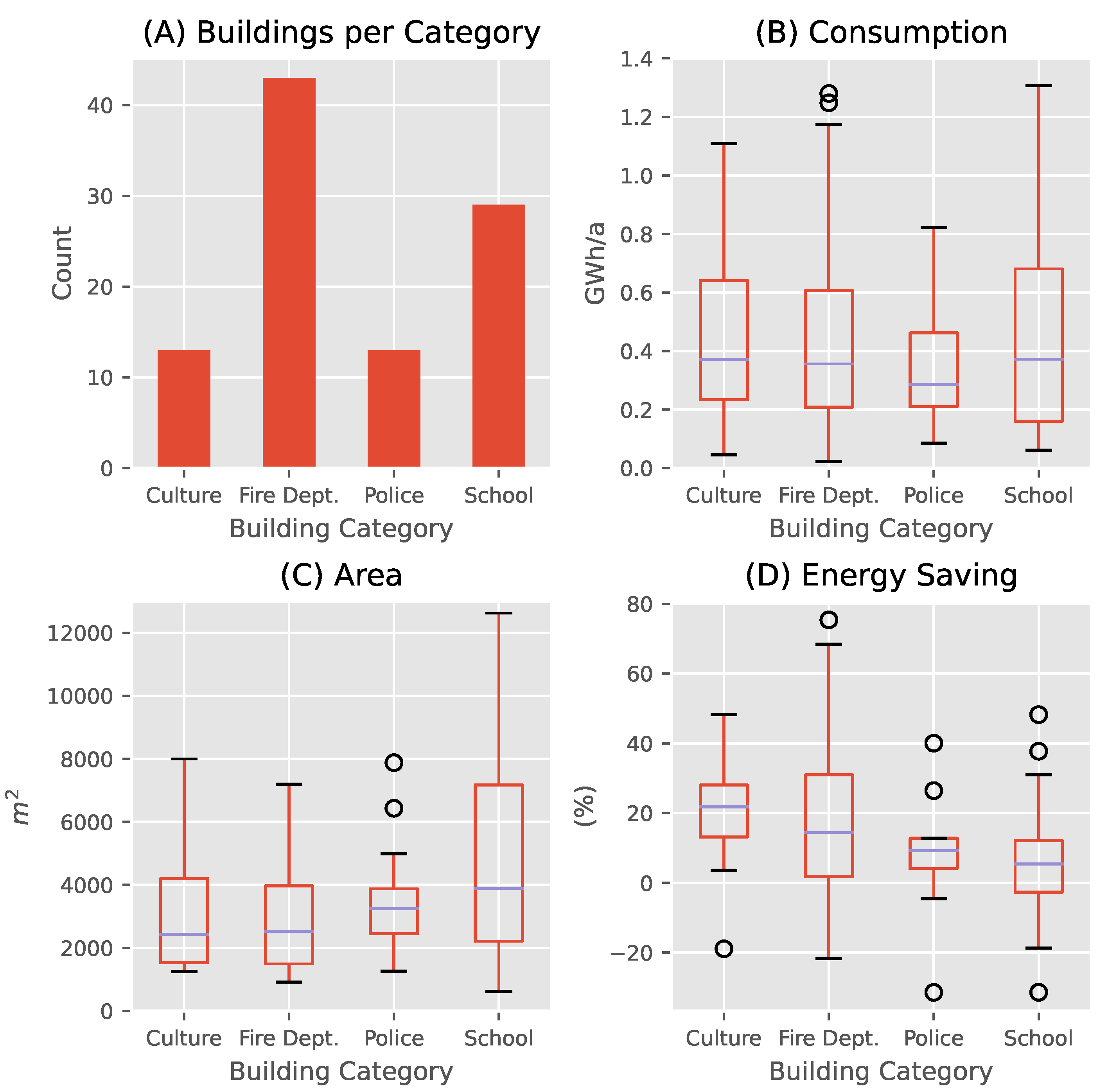
3. Data Set
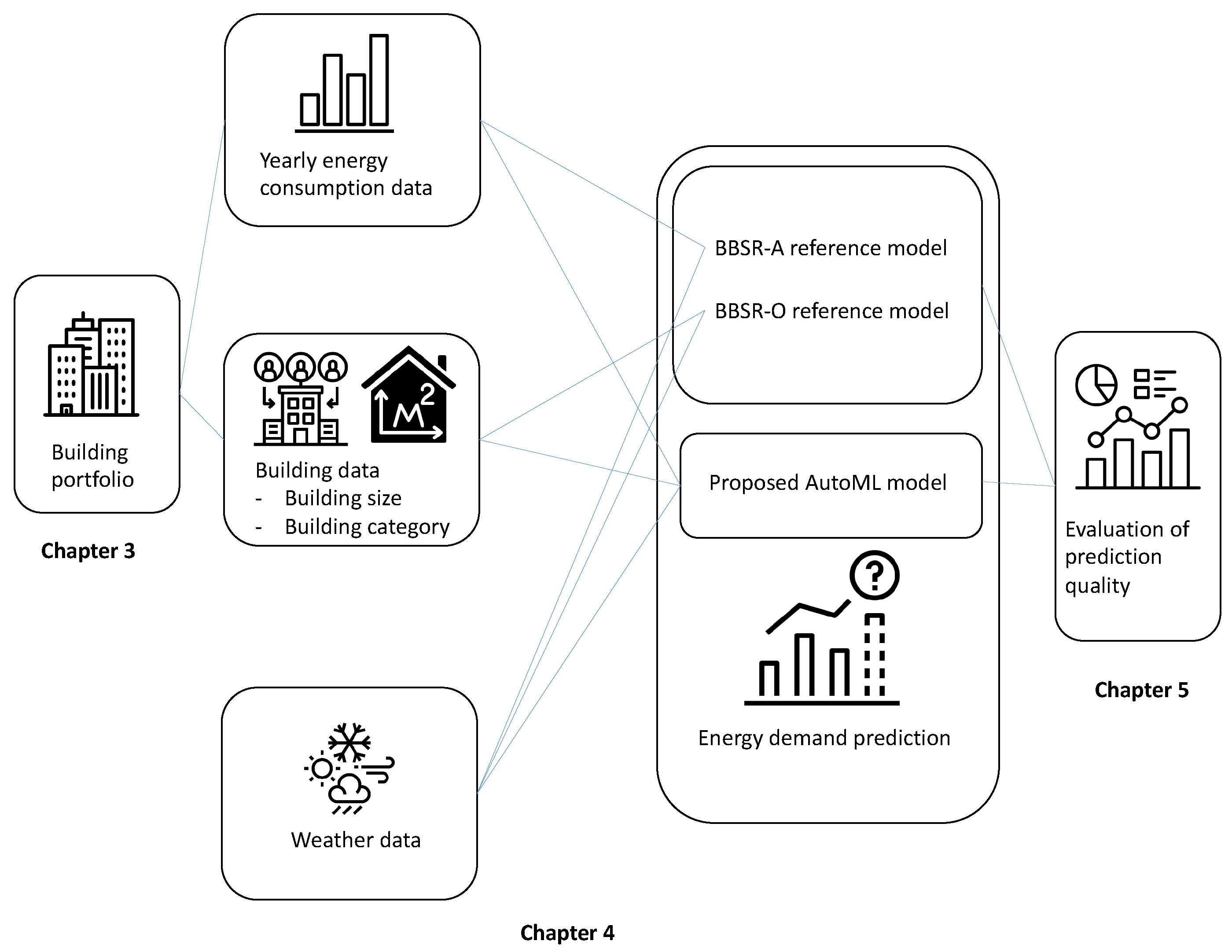
4. Methods
4.1. Linear BBSR Model
4.2. Adapted BBSR Model (BBSR-A)
4.3. Optimized BBSR Model
4.4. Automated Machine Learning Model
4.5. Modeling Seasonal Climate Changes
4.5.1. Correcting for Seasonal Climate Changes
4.5.2. Sampling Realistic Climate Characteristics for Forecasts
5. Results
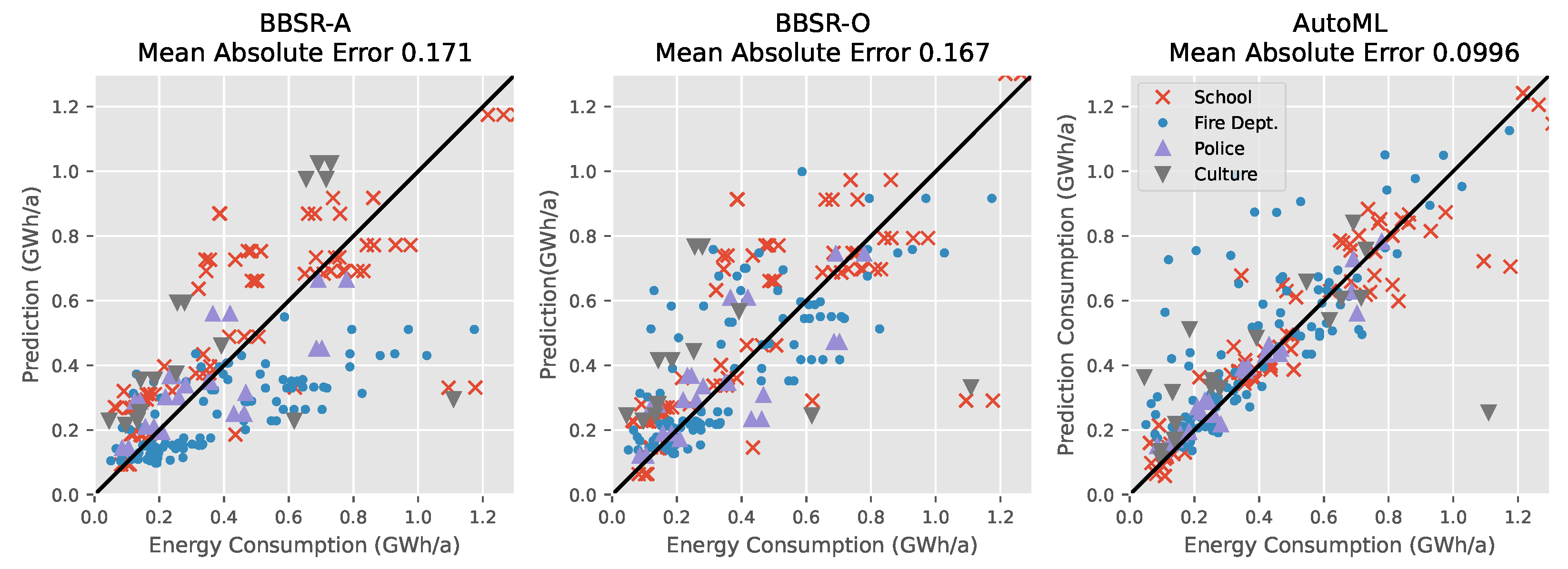
5.1. Modeling Energy Consumption
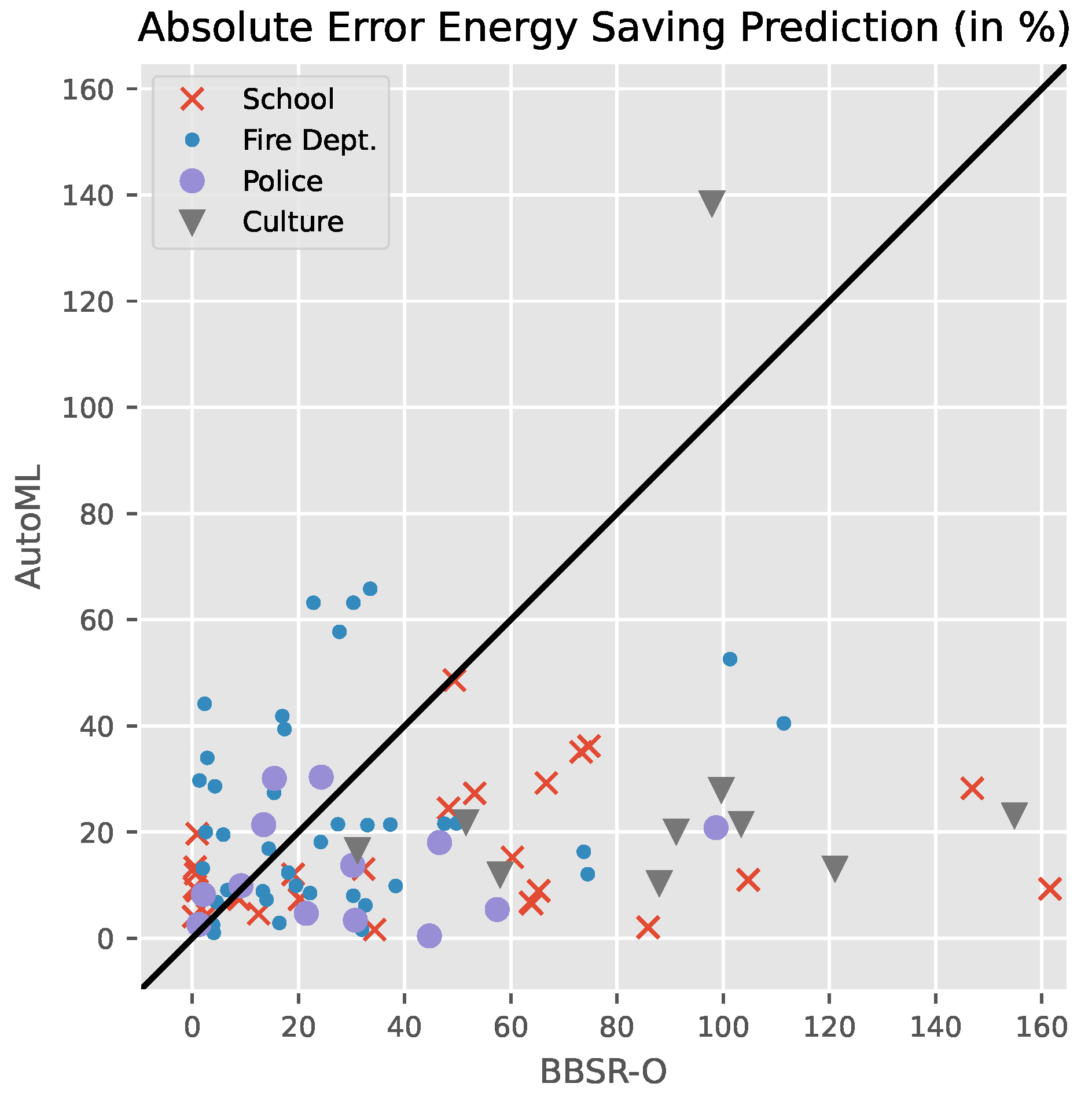
5.2. Modeling Energy Savings
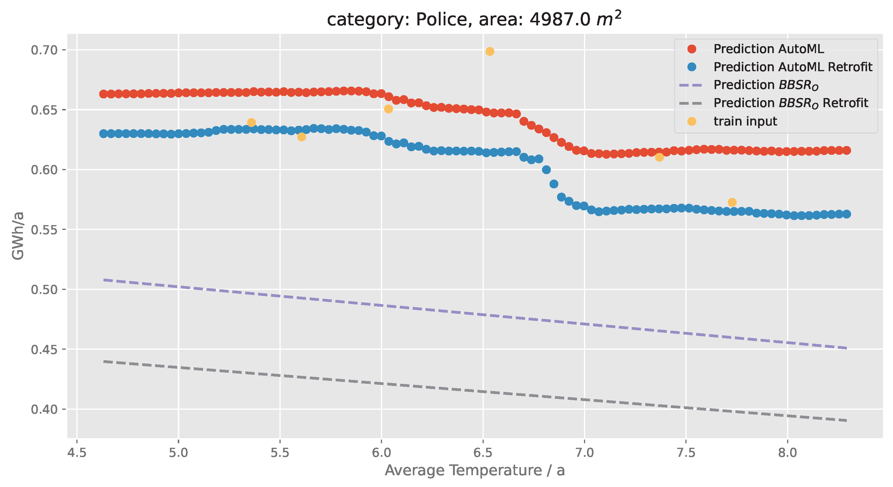
5.3. Modeling Energy Consumption for Individual Buildings
6. Conclusions
Author Contributions
Funding
Data Availability Statement
Acknowledgments
Conflicts of Interest
References
- U.S. Energy Information Administration. Energy Statistics; U.S. Energy Information Administration: Washington, DC, USA, 2023.
- Lee, J.; Shepley, M.M.; Choi, J. Exploring the effects of a building retrofit to improve energy performance and sustainability: A case study of Korean public buildings. J. Build. Eng. 2019, 25, 100822. [Google Scholar] [CrossRef]
- Fathi, S. Machine learning applications in urban building energy performance forecasting: A systematic review. Renew. Sustain. Energy Rev. 2020, 133, 110287. [Google Scholar] [CrossRef]
- Chen, Y.; Hong, T. Impacts of building geometry modeling methods on the simulation results of urban building energy models. Appl. Energy 2018, 215, 717–735. [Google Scholar] [CrossRef]
- Fonseca, J.A.; Schlueter, A. Integrated model for characterization of spatiotemporal building energy consumption patterns in neighborhoods and city districts. Appl. Energy 2015, 142, 247–265. [Google Scholar] [CrossRef]
- Reinhart, C.F.; Davila, C.C. Urban building energy modeling—A review of a nascent field. Build. Environ. 2016, 97, 196–202. [Google Scholar] [CrossRef]
- Chalal, M.L.; Benachir, M.; White, M.; Shrahily, R. Energy planning and forecasting approaches for supporting physical improvement strategies in the building sector: A review. Renew. Sustain. Energy Rev. 2016, 64, 761–776. [Google Scholar] [CrossRef]
- Zhao, H.x.; Magoulès, F. A review on the prediction of building energy consumption. Renew. Sustain. Energy Rev. 2012, 16, 3586–3592. [Google Scholar] [CrossRef]
- Seyedzadeh, S.; Rahimian, F.P.; Glesk, I.; Roper, M. Machine learning for estimation of building energy consumption and performance: A review. Vis. Eng. 2018, 6, 5. [Google Scholar] [CrossRef]
- Elbeltagi, E.; Wefki, H. Predicting energy consumption for residential buildings using ANN through parametric modeling. Energy Rep. 2021, 7, 2534–2545. [Google Scholar] [CrossRef]
- Truong, N.S.; Ngo, N.T.; Pham, A.D. Forecasting time-series energy data in buildings using an additive artificial intelligence model for improving energy efficiency. Comput. Intell. Neurosci. 2021, 2021, 6028573. [Google Scholar] [CrossRef] [PubMed]
- Olu-Ajayi, R.; Alaka, H.; Sulaimon, I.; Sunmola, F.; Ajayi, S. Building energy consumption prediction for residential buildings using deep learning and other machine learning techniques. J. Build. Eng. 2022, 45, 103406. [Google Scholar] [CrossRef]
- Ma, Z.; Ye, C.; Li, H.; Ma, W. Applying support vector machines to predict building energy consumption in China. Energy Procedia 2018, 152, 780–786. [Google Scholar] [CrossRef]
- Zhang, X.; Zhang, J.; Zhang, J.; Zhang, Y. Research on the combined prediction model of residential building energy consumption based on random forest and BP neural network. Geofluids 2021, 2021, 7271383. [Google Scholar] [CrossRef]
- Wang, Z.; Wang, Y.; Zeng, R.; Srinivasan, R.S.; Ahrentzen, S. Random Forest based hourly building energy prediction. Energy Build. 2018, 171, 11–25. [Google Scholar] [CrossRef]
- Liu, Y.; Chen, H.; Zhang, L.; Feng, Z. Enhancing building energy efficiency using a random forest model: A hybrid prediction approach. Energy Rep. 2021, 7, 5003–5012. [Google Scholar] [CrossRef]
- Rätz, M.; Javadi, A.P.; Baranski, M.; Finkbeiner, K.; Müller, D. Automated data-driven modeling of building energy systems via machine learning algorithms. Energy Build. 2019, 202, 109384. [Google Scholar] [CrossRef]
- Bundesministerium des Innern, für Bau und Heimat. Bekanntmachung der Regeln für Energieverbrauchswerte und der Vergleichswerte im Nichtwohngebäudebestand. Available online: https://geg-info.de/geg/210503_bmwi_bmi_regeln_energieverbrauchskennwerte_nichtwohnbestand.pdf (accessed on 1 April 2021).
- Erickson, N.; Mueller, J.; Shirkov, A.; Zhang, H.; Larroy, P.; Li, M.; Smola, A. AutoGluon-Tabular: Robust and Accurate AutoML for Structured Data. arXiv 2020, arXiv:2003.06505. [Google Scholar]
- Deutscher Wetterdienst. Klimafaktoren (KF) für Energieverbrauchsausweise; Deutscher Wetterdienst: Offenbach am Main, Germany, 2020. [Google Scholar]


| Category | ECO Factor | ||
|---|---|---|---|
| Police Stations | 52.4 | 7.4 | 0.86 |
| Fire Stations | 50.8 | 7.1 | 0.86 |
| Schools | 49.3 | 22.4 | 0.96 |
| Cultural | 55.9 | 7.5 | 0.87 |
| Year | KF | TM | SO | NM | FM | RFM |
|---|---|---|---|---|---|---|
| 2021 | 1.08 | 5.72 | 3.31 | 6.39 | 4.29 | 82.02 |
| 2020 | 1.20 | 7.37 | 4.45 | 5.67 | 4.38 | 76.78 |
| 2019 | 1.19 | 7.01 | 3.87 | 5.59 | 4.53 | 78.50 |
| 2018 | 1.17 | 5.15 | 3.53 | 5.72 | 4.39 | 80.24 |
| 2017 | 1.11 | 6.19 | 2.98 | 6.09 | 4.50 | 83.31 |
| 2016 | 1.10 | 5.19 | 3.01 | 6.06 | 4.23 | 81.88 |
| 2015 | 1.13 | 7.56 | 4.24 | 5.53 | 4.54 | 80.07 |
| Building Features | Climate Features (Yearly Aggregates) |
|---|---|
| Area in | Outside temperature (2 m above ground) |
| Building category | Sum of sunshine hours |
| Energy efficiency measure (True or False) | Cloud cover |
| Consumption in past years | Wind |
| Humidity |
| MAE BBSR-A | MAE BBSR-O | MAE AutoML | |
|---|---|---|---|
| School | 156,697 | 150,102 | 71,109 |
| Fire Dept. | 156,521 | 122,545 | 106,553 |
| Police | 106,684 | 103,978 | 38,904 |
| Culture | 375,970 | 541,350 | 236,521 |
| Mean | 198,968 | 229,494 | 113,272 |
| BBSR-O | BBSR-A | AutoML | |
|---|---|---|---|
| School | 45 | 52 | 14 |
| Fire Dept. | 24 | 28 | 22 |
| Police | 30 | 32 | 12 |
| Culture | 108 | 70 | 29 |
| Mean | 41 | 40 | 19 |
Disclaimer/Publisher’s Note: The statements, opinions and data contained in all publications are solely those of the individual author(s) and contributor(s) and not of MDPI and/or the editor(s). MDPI and/or the editor(s) disclaim responsibility for any injury to people or property resulting from any ideas, methods, instructions or products referred to in the content. |
© 2023 by the authors. Licensee MDPI, Basel, Switzerland. This article is an open access article distributed under the terms and conditions of the Creative Commons Attribution (CC BY) license (https://creativecommons.org/licenses/by/4.0/).
Share and Cite
Biessmann, F.; Kamble, B.; Streblow, R. An Automated Machine Learning Approach towards Energy Saving Estimates in Public Buildings. Energies 2023, 16, 6799. https://doi.org/10.3390/en16196799
Biessmann F, Kamble B, Streblow R. An Automated Machine Learning Approach towards Energy Saving Estimates in Public Buildings. Energies. 2023; 16(19):6799. https://doi.org/10.3390/en16196799
Chicago/Turabian StyleBiessmann, Felix, Bhaskar Kamble, and Rita Streblow. 2023. "An Automated Machine Learning Approach towards Energy Saving Estimates in Public Buildings" Energies 16, no. 19: 6799. https://doi.org/10.3390/en16196799
APA StyleBiessmann, F., Kamble, B., & Streblow, R. (2023). An Automated Machine Learning Approach towards Energy Saving Estimates in Public Buildings. Energies, 16(19), 6799. https://doi.org/10.3390/en16196799