Application of the Energy Efficiency Mathematical Model to Diagnose Photovoltaic Micro-Systems

Abstract

The intensive development of photovoltaic (PV) micro-systems contributes to increased interest in energy efficiency and diagnosing the condition of such solutions. Optimizing system energy efficiency and servicing costs are particularly noteworthy among the numerous issues associated with this topic. This research paper addresses the easy and reliable diagnosis of PV system malfunctions. It discusses the original PV system energy efficiency simulation model with proprietary methods for determining total solar irradiance on the plane of cells installed at any inclination angle and azimuth, as well as PV cell temperature and efficiency as a function of solar irradiance. Based on this simulation model, the authors developed procedures for the remote diagnosis of PV micro-systems. Verification tests covered two independent PV systems over the period from April 2022 to May 2023. The obtained results confirm the high credibility level of both the adopted energy efficiency simulation model and the proposed method for diagnosing PV system functional status.

1. Introduction

The global capacity of PV systems has exceeded 1 TWp and continues to rapidly grow, with a significant share of micro-systems. For example, the Institute for Renewable Energy report claims that the PV capacity in Poland installed at the end of March 2023 exceeded 13 GW, including a 74% share of prosumer micro-systems. Furthermore, studies indicate a reduced micro-system efficiency relative to professional PV power plants. Research conducted in France and Belgium on more than 10,000 systems has demonstrated lower micro-system efficiency by 16% [1]. Therefore, optimizing the energy efficiency of PV micro-systems, which should be taken into account not only at the engineering stage but also during operation, is an important aspect [2,3,4]. Maintaining the highest efficiency level of PV systems throughout their operation requires reliable and rapid servicing and diagnosing [5,6,7]. In light of the territorial dispersion of micro-systems (with most of them located on buildings), methods that involve systematic human-conducted equipment inspections are costly [8,9,10]. Therefore, remote diagnosis is the basic technique [11,12,13,14].

Remote diagnosis primarily employs measurement data from devices built into photovoltaic systems, such as inverters and power optimizers. In addition, it also utilizes data from temporarily or permanently installed auxiliary equipment. This includes weather stations and cameras. The source literature contains publications that preview various diagnostic methods, which analyse thermal imaging camera images [15,16,17,18,19,20,21]. The article reviews methods of identifying mismatch errors related to photovoltaic modules based on analysing temperature distribution obtained through thermography [15] or identifying hot spots, penumbra and other minor defects. There are also mixed methods that combine thermal imaging with machine learning. This enables distinguishing between visual damage that hinders the operation and reduces PV module durability or automatic system inspections throughout its entire life cycle. Because the maintenance-free version of these methods requires cameras monitoring all PV system cells, they are relatively expensive. Moreover, they primarily enable the detection of hot spots, allowing to determine an energy efficiency deterioration to a lower degree. There have also been studies based on the method of comparing neighbouring systems [22], large-scale dispersion [23] or referring to such numerous, different models [24]. The largest group includes papers describing the diagnosis of photovoltaic systems based on inverter and weather station data using artificial intelligence, particularly machine learning methods [25,26,27,28,29,30,31,32,33,34,35,36]. They are widely discussed in the source literature and usually provide good diagnostic results; however, they require a specific set of training data for each PV system unit. In the latest literature, you can also find the use of mathematical models for: the optimization of renewable energy systems taking into account several sources [37,38], business models facilitating decision-making in the field of PV microgrids [39], the modeling of photovoltaic cells as semiconductor materials [40,41,42] or maximum power point optimization (MPPT) [43,44]. The aforementioned numerous studies are aimed at developing methods for the remote, rapid and reliable diagnosis of actual photovoltaic micro-systems, which is economically justified.

Therefore, the authors of the article proposed a diagnostic method based on comparing the actual PV micro-system efficiency provided by inverter applications with the theoretical efficiency, calculated using an original simulation model. The parametric simulation model would only employ meteorological data (solar irradiance, temperature, wind speed), as well as PV system technical and structural parameters. This led to an attempt at developing a standardized energy efficiency coefficient (SEEC), which is universal for each PV system. This means that making a reliable diagnosis of the occurrence of a failure that reduces the energy efficiency of a given PV system will not require previous tests of this device in a state of fitness. The coefficient employed within the tests may spread over custom time periods, with daily periods adopted for the study.

The individual chapters of the article discuss:

• The PV system efficiency simulation model;
• description of the tests covering two PV systems;
• application of the standardized energy efficiency coefficient for diagnosing a PV system.

The objective of the publication is to demonstrate the usefulness of the presented method for remote energy efficiency assessment and diagnosing actual photovoltaic micro-systems, as well as its competitiveness in terms of credibility, costs and deployment simplicity.

2. Mathematical Model of Solar Irradiance on PV System Cell Plane

The target parameter employed for the diagnosis process is the PV standardized efficiency index (SEI). It requires accurately simulating the waveform of the theoretical instantaneous power of a diagnosed PV system. The power of photovoltaic (PV) cells is calculated as per the Formula (1) [45,46,47,48,49].

$$P_{PV}={\eta }_{PV}·A_{PV}·G_{PV},$$

(1)

where P_PV—power generated by a PV system [W], η_PV—PV module efficiency, A_PV—cell active surface [m²], G_PV—instantaneous values of solar irradiance on the surface of a photovoltaic module [W/m²].

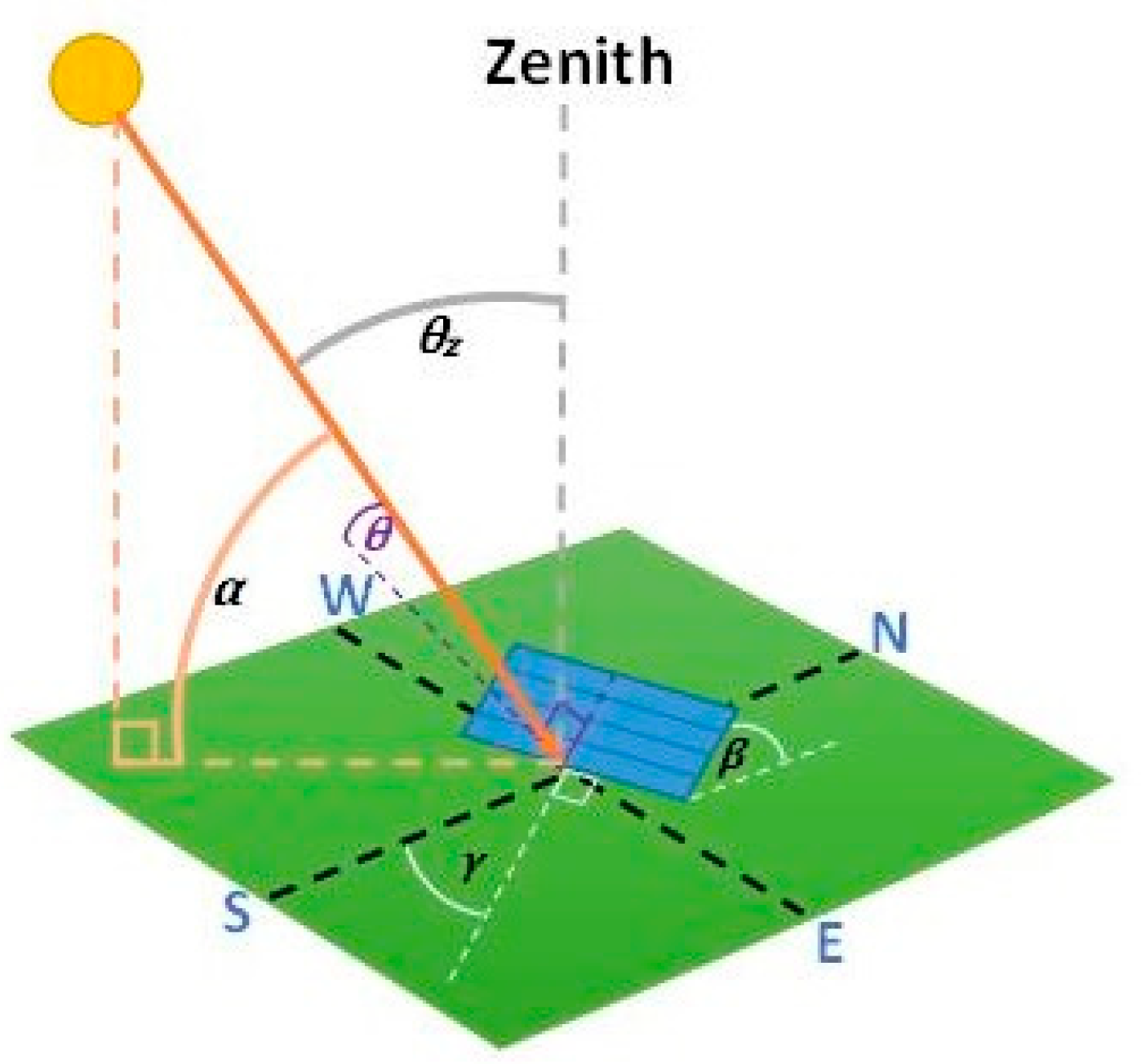
System area A_PV is known, while its efficiency depends on PV cell technical parameters and weather conditions. This will be more thoroughly explored in the chapter. The instantaneous power graph waveform is most impacted by solar irradiance of the cell plane G_PV and is the most variable factor. Furthermore, cell planes in building systems, prosumer micro-systems in particular, are generally set at various inclination angles and azimuths. A majority of basic meteorological devices only measure the total solar irradiance of a vertical plane, parallel to the Earth’s surface, and determining G_PV requires complex computations [50]. A diagram in Figure 1 helps to illustrate a general model of solar radiation after it passes the Earth’s atmosphere.

Physical phenomena, mainly dispersion, diffraction and absorption within various strata of the atmosphere, including clouds, lead to reduced intensity and a modification of its structure. Therefore, total irradiance on a plane parallel to the Earth’s surface is determined using the Formula (2) [51,52,53]:

$$G_S=G_B+G_{RI}+G_{RO}+G_{RH}+G_{OD},$$

(2)

where G_S—total solar irradiance [W/m²], G_B—direct solar irradiance [W/m²], G_RI—diffuse, isotropic solar irradiance [W/m²], G_RO—diffuse, circumsolar solar irradiance [W/m²], G_RH—diffuse, brightening solar irradiance horizon [W/m²], G_OD—reflected solar irradiance [W/m²].

Calculating solar irradiance on the surface of a PV cell inclined relative to the Earth’s plane using the Formula (2) would be complex and is not expedient. In addition to direct irradiance (G_B) of vector value, all other components are of isotropic nature and, therefore, the Formula (2) can be simplified to the Formula (3).

$$G_S=G_B+G_R,$$

(3)

where G_S—total solar irradiance [W/m²], G_B—direct solar irradiance [W/m²], G_R—diffuse, isotropic solar irradiance [W/m²].

The measurement results for total irradiance on a plane parallel to the Earth’s surface G_S and diffuse irradiance G_R enable calculating direct irradiance on the plane parallel to the Earth’s surface G_B (4).

$$G_B=G_S-G_R,$$

(4)

Next, one can calculate direct irradiance on the plane inclined at any angle β and rotated southwards at an angle γ using the Formula (5) [51,52], as shown in Figure 2.

$$G_{BP}=G_B\frac{\cos \theta }{\sin \alpha },$$

(5)

where: G_BP—directional irradiance on an inclined and rotated plane [W/m²], θ—direct solar radiation angle of incidence on a surface with any inclination relative to the horizontal and any azimuth [°], α—Sun’s angle of elevation [°].

This enables calculating total irradiance G_PV on a plane inclined at an angle β and rotated by an angle γ as per the Formula (6).

$$G_{PV}=G_{BP}+G_R,$$

(6)

By applying the Formulas (4)–(6), we obtain the Formula (7)

$$G_{PV}=\left(G_S-G_R\right)\frac{\cos \theta }{\sin \alpha }+G_R,$$

(7)

where: G_PV—total irradiance on a plane inclined at an angle β and rotated by an angle γ [W/m²],

Moreover, sin α is defined by the Formula (8) [52,53]

$$\sin \alpha =\left(\cos \phi \cos \delta \cos \omega +\sin \phi \sin \delta \right),$$

(8)

where: φ—latitude [°], δ—solar declination [°], ω—Sun’s hour angle [°].

Whereas cos θ is defined by the Formula (9)

$$\begin{gathered} \cos \theta =\sin \delta \left(\sin \phi \cos \beta -\cos \phi \sin \beta \cos \gamma \right)+\cos \delta ·(\cos \phi \cos \beta \cos \omega + \\ \sin \beta \sin \phi \cos \gamma \cos \omega +\sin \beta \sin \gamma \sin \omega ), \end{gathered}$$

(9)

where: β—plane inclination angle (angle between the horizon and receiver) [°], γ—azimuth angle (angle between the receiver and southwards direction) [°].

The solar declination appearing in Formulas (8) and (9) is calculated according to Formula (10) and the Sun’s hour angle is calculated according to Formula (11)

$$\delta =23.45°\sin \frac{360°·\left(284+d\right)}{365},$$

(10)

where: d—numbered day of the year

$$\omega =15\left(t-12\right)+\lambda -30,$$

(11)

where: t—time in hours, assuming that t = 0 is midnight in the UTC+02:00 time zone, λ—longitude.

After applying Formulas (8) and (9), the instantaneous diffuse irradiance value remains the only unknown in the Formula (7). Because diffuse irradiance is not usually measured, it is calculated based on Formula (12) for the purposes of the simulation model.

$$\begin{gathered} f\left(x,y\right)=2.9605494704543585+0.5377862858796892x+ \\ 0.06004726482252161y-0.0026910268413485984x^2+ \\ 0.0019042965793833588xy-0.00017756733488081473y^2+ \\ 3.042172248692004{·10}^{-6}{x}^3-3.178624909592273{·10}^{-6}{x}^{2}y+ \\ 8.214875913822176{·10}^{-7}x{y}^2-1.0830525365875006{·10}^{-7}{y}^3, \end{gathered}$$

(12)

where: f(x,y)—G_R diffuse solar radiation x—G_CP, measured total irradiance [W/m²], y—G_CT, theoretical total irradiance [W/m²].

Formula (12) has been developed as part of work on the optimal method for calculating diffuse irradiance based on the studies presented in [50], which also thoroughly describes formulas for calculating theoretical total irradiance G_CT.

By substituting the results of calculations from Formulas (8) and (9), and the instantaneous diffuse irradiance G_R calculated using Formula (12) to Formula (7), the authors obtained an instantaneous irradiance on the PV cell plane. The outcome was a mathematical model that enables calculating instantaneous irradiance on the PV cell plane G_R based on PV system structural data, its geographical location and measured total irradiance on the plane parallel to the Earth’s surface. Therefore, only PV module efficiencies are missing to calculate power waveforms according to the Formula (1).

3. PV Cell Efficiency Mathematical Model

Efficiency, defined as the ratio of energy produced to solar radiation energy falling on a PV cell, depends on the temperature of the semi-conductor structure and the solar irradiance value. Therefore, PV cell energy efficiency depends on the execution technology, which is reflected by the technical parameters of the system structure and weather conditions [51,52,53]. In addition to the technical conditions, which should be variable over time, efficiency is also impacted by such physical phenomena as temperature and the insolation of PV cells, which are variable over time. Therefore, instantaneous PV cell efficiency can be expressed using the Formula (13).

$${\eta }_{PV}={\eta }_{STC}·{\eta }_G\left(G_{PV}\right)·{\eta }_t\left(t\right),$$

(13)

where η_PV—instantaneous PV cell efficiency, η_STC—nominal PV cell efficiency under STC conditions, η_G—standardized PV cell efficiency function depending on solar radiation intensity, η_t—standardized efficiency function depending on the temperature of the PV cell.

Nominal module efficiency η_STC is determined by the manufacturer under STC (Standard Test Conditions); i.e., a solar intensity of 1000 W/m² and a module temperature of 25 °C.

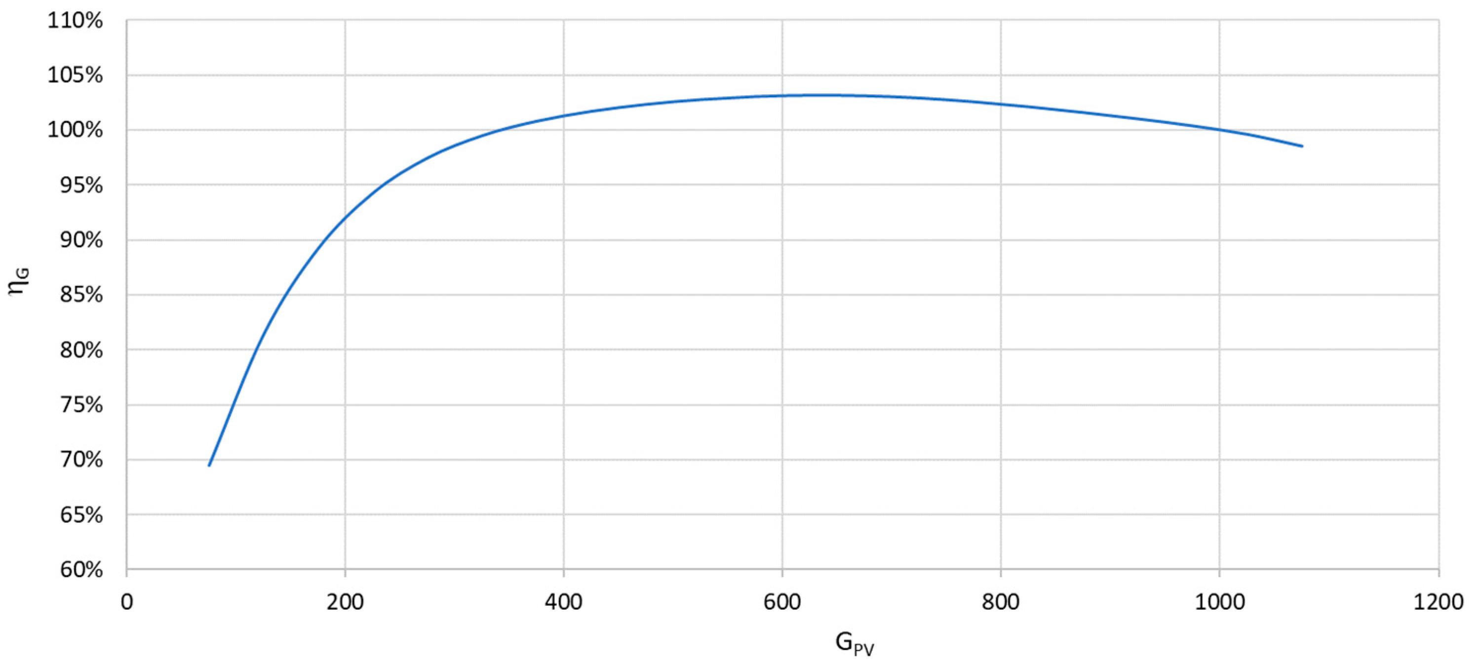
The standardized PV cell efficiency function η_G is dependent on solar irradiance [54,55,56]. This relationship was determined based on the results of tests covering five photovoltaic systems equipped with mono-crystalline cells. The approximate function was determined by Formula (14), and its waveform is shown in Figure 3.

$$\begin{gathered} {\eta }_G=-6.103·{10}^{-18}·{G_{PV}}^6+2.527·{10}^{-14}·{G_{PV}}^5-4.262·{10}^{-11}·{G_{PV}}^4+ \\ 3.76·{10}^{-8}·{G_{PV}}^3--1.872·{10}^{-5}·{G_{PV}}^2+5.142·{10}^{-3}·G_{PV}+0.4002, \end{gathered}$$

(14)

where η_G—standardized PV cell efficiency function, G_PV—solar irradiance.

The last element to be determined in Formula (13) is η_t the standardized efficiency function, depending on the temperature of the PV cell. The efficiency of all PV cell types depends on temperature, while in the case of mono-crystalline cells, this relationship is relatively strong and should be taken into account when simulating the efficiency of photovoltaic systems [55,56,57]. It can be determined using the Formula (15).

$${\eta }_t=1+{\beta }_t\left(t_{PV}-t_{STC}\right),$$

(15)

where η_t—standardized efficiency function depending on the temperature of the PV cell, β_t—temperature coefficient of maximum PV cell power, t_PV—PV cell temperature, t_STC—temperature under STC (25 °C).

Formula (15) employs the maximum power temperature coefficient, since PV systems should operate at a maximum power point (MPP). The coefficient β_t is directly determined by the manufacturer, and mono-crystalline silicon cells usually range from—0.4%/°C to—0.3%/°C.

Formula (15) also includes t_PV, which is the PV cell temperature, and more precisely, the cell semi-conductor structure temperature. This temperature is not measured, and the cell housing temperature is also usually not measured. This temperature can be measured in the devices near PV cells (e.g., power optimizers), but in such a case, the devices cooperating with PV cells provide plenty of diagnostic information and the application of diagnostic methods presented herein is not expected. It was assumed that the developed simulation model would only be applied in systems comprising PV cell chains without optimizers or microinverters. In such a situation, the PV cell temperature should be determined based on meteorological measurements in the vicinity of the system, as well as on structural properties.

In order to determine the temperature, the authors analysed employed PV cell semi-conductor structure temperature calculation models. One of the most popular among them is the empirical formula described by Equation (16), which is based on basic climate parameters; i.e., solar irradiance, wind speed and ambient temperature [58].

$$t_{PV}=G_{PV}·e^{a+b·V_w}+t_e,$$

(16)

where t_PV—PV cell temperature °C, G_PV—solar irradiance on the PV cell surface W/m², V_w—wind speed, t_e—PV system ambient temperature, a and b—empirical coefficients depending on the PV system installation method and execution technology.

Examples of a and b coefficients for different PV cell types and installation models are shown in

Table 1. Values of a and b coefficients employed in Equation (16) [58].

PV Module Type	Installation Method	a	b
Glass/cell/glass	Full ventilation	−3.74	−0.0594
Glass/cell/glass	At the roof slope	−2.98	−0.0471
Glass/cell/polymer coating	Full ventilation	−3.56	−0.0750
Glass/cell/polymer coating	Rear surface insulation	−2.81	−0.0455
Polymer/PV-thin film/steel	Full ventilation	−3.58	−0.1130

.

Another recognized model that enables estimating PV cell temperature is the Servant temperature model, which takes into account parameters such as ambient temperature, solar irradiance, module electrical efficiency or wind speed [59], and is described by Equation (17).

$$t_{PV}=t_e+\alpha G_{PV}\left(1+\beta t_e\right)\left(1-\gamma V_w\right)\left(1-1.053{\eta }_{STD}\right),$$

(17)

where t_PV—PV cell temperature °C, G_PV—solar irradiance on the surface of a PV cell W/m², V_w—wind speed, t_e—PV system ambient temperature, η_STC—standardized PV cell temperature under STC conditions, α, β, γ—constant, their values are α = 0.0138, β = 0.031 and γ = 0.042, respectively.

The Servant temperature model was determined based on analysing temperature-dependent graphical correlations relative to solar irradiance. A correlation degree in the range of 0.69 ÷ 0.89 was obtained. The values of the α, β and γ constants were empirically determined by the model’s author under conditions of a constant wind speed of 1 m/s. The accuracy may be lower for other speed values.

Another considered model is the Davis, Dougherty and Fanney model presented by Formula (18) [59]. It is primarily based on the coefficients specified under NOCT conditions; i.e., nominal operating cell temperature. Furthermore, it utilizes meteorological data such as ambient temperature and solar irradiance.

$$t_{PV}=t_e+\frac{G_{PV}}{G_{NOCT}}\left(t_{PVNOCT}-t_{eNOCT}\right)\left(1-\frac{{\eta }_{STC}}{\tau ·\alpha }\right),$$

(18)

where t_PV—PV cell temperature °C, G_PV—solar irradiance on the surface of a PV cell W/m², t_e—PV system ambient temperature, η_STC—nominal PV cell efficiency under STC conditions, G_NOCT—solar irradiance under NOCT conditions [800 W/m² ], t_PVNOCT—PV cell under NOCT conditions [°C], t_eNOCT—ambient temperature under NOCT conditions [20 °C], τ—transmittance, α—absorptiveness.

Formula (18) was developed based on tests involving photovoltaic modules within free-standing systems, normally oriented to solar noon. There is also a more extensive dependence (19), the so-called Homer formula based on similar data as Formula (18). In addition, it only contains the temperature power coefficient and enables determining instantaneous cell temperature based on the results of the test conducted under NOCT and STC conditions [60].

$$t_{PV}=\frac{t_e+\left(t_{PVNOCT}-t_{eNOCT}\right)\left(\frac{G_{PV}}{G_{NOCT}}\right)\left[1-\frac{{\eta }_{STC}\left(1-{\alpha }_p{t}_{STC}\right)}{\tau ·\alpha }\right]}{1+\left(t_{NOCT}-t_{eNOCT}\right)\left(\frac{G_{PV}}{G_{NOCT}}\right)\left(\frac{{\alpha }_p{\eta }_{STC}}{\tau ·\alpha }\right)},$$

(19)

where t_PV—PV cell temperature °C, G_PV—solar irradiance on the surface of a PV cell W/m², t_e—PV system ambient air temperature, η_STC—nominal PV cell efficiency under STC conditions, G_NOCT—solar irradiance under NOCT conditions [800 W/m²], t_PVNOCT—PV cell temperature under NOCT conditions [°C], t_eNOCT—ambient temperature under NOCT conditions [20 °C], τ—transmittance, α—absorptiveness, α_p—maximum power temperature coefficient.

The David Faiman model, which determines the PV cell temperature based on the heat exchange concept, was also considered [61,62]. The model is represented by Formula (20).

$$t_{PV}=t_e+\frac{G_{STC}}{U_0+U_1·V_w},$$

(20)

where t_PV—PV cell temperature °C, G_STC—solar irradiance under STC conditions 1000 W/m², V_w—wind speed, t_e—PV system ambient air temperature, U₀—heat transfer constant W/m² K, U₁—convective heat exchange constant W/m³sK.

The U₀ and U₁ constants were empirically determined by the author of the model through measuring solar irradiance on the PV module surface, and the wind speed and temperature of seven PV module types. The U₀ constant values ranged from (23.5 ÷ 26.5) W/m² K and U₁ (6.25 ÷ 7.68) W/m³ sK.

The last model taken into account was the one employed by PVsyst in their software for modelling photovoltaic system efficiency. The implemented Formula (21) was very similar to the one proposed in the Faiman model.

$$t_{PV}=t_e+G_{STC}·\frac{\alpha \left(1-{\eta }_{STC}\right)}{U_0+U_1·V_w},$$

(21)

where t_PV—PV cell temperature °C, G_STC—solar irradiance under STC conditions 1000 W/m², V_w—wind speed, t_e—PV system ambient air temperature, U₀—heat transfer constant W/m² K, U₁—convective heat exchange constant W/m³sK, η_STC—nominal efficiency of the PV cell under STC conditions.

This model employs default values of the U₀ and U₁ constants, which are: for free-standing systems: U₀ = 29 W/m² K, U₁ = 0 W/m³ sK, while for systems located at the roof slope: U₀ = 15 W/m² K, U₁ = 0 W/m³ sK. It should be noted that default U₁ = 0 W/m³ sK; therefore, the dependence of temperature on wind speed responsible for cooling PV modules is not assumed.

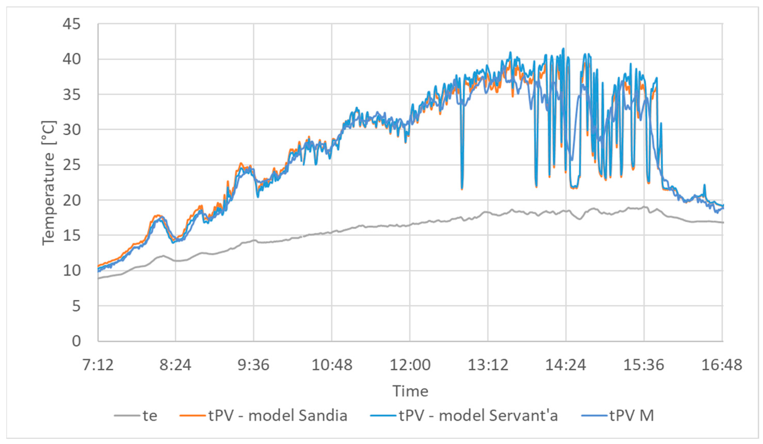
Parallel meteorological and temperature measurements covering selected PV cells were conducted for five systems in the years 2020–2023 to select the optimal dependence on PV cell temperature. An indirect measurement of the cell semi-conductor structure temperature was conducted using thermal imaging cameras or a four-channel temperature recorder. The measured temperature waveforms were adopted as references, and the mean and mean square differences between the calculated and measured values were calculated for all models defined by the Formulas (16)–(21). The analysis covered 50 time periods from 5 to 12 h. The best results were obtained for models defined by Formulas (16) and (17). With appropriately selected coefficients, the authors obtained a mean value of the waveform difference below 0.1 °C and a standard mean square deviation of 2.5 °C. Examples of measured temperature value waveforms, calculated based on the Sandia and Servant models, are shown in Figure 4 and Figure 5.

When comparing temperature waveforms, one can notice the convergence of their value trend, especially under continuous and good insolation. The differences between instantaneous values under dynamically variable insolation conditions are significant because all computational temperature models fail to take PV cell thermal inertia into account. Despite the considerable difference in instantaneous values, the differences in mean values for hourly or longer periods are small. Therefore, Formulas (16) and (17) can be employed when simulating the daily energy efficiency and provide good accuracy.

It should be noted that the aforementioned tests and analyses of different variants were only aimed at comparing existing solutions and selecting an optimal PV cell temperature computational model. Due to the accuracy, the criteria were satisfied by at least two formulas, but Formula (16) was chosen to be applied in the PV cell energy efficiency simulation model since it enabled simpler implementation. After substituting (15), the authors obtained the final formula for standardized temperature efficiency (22).

$${\eta }_t=1+{\beta }_t\left(G_{PV}·e^{a+b·V_w}+t_e-t_{STC}\right),$$

(22)

where η_t—standardized efficiency function depending on the temperature of a PV cell, β_t—PV cell maximum power temperature coefficient, G_PV—solar irradiance on the surface of a PV cell, V_w—wind speed, t_e—PV cell ambient air temperature, a and b—empirical coefficients depending on the installation method and execution technology, t_STC—PV cell temperature under STC conditions (25 °C).

After substituting Formula (13), values calculated using Formulas (14) and (22) give results in the PV cell instantaneous efficiency.

4. Simulating PV System Power Waveforms

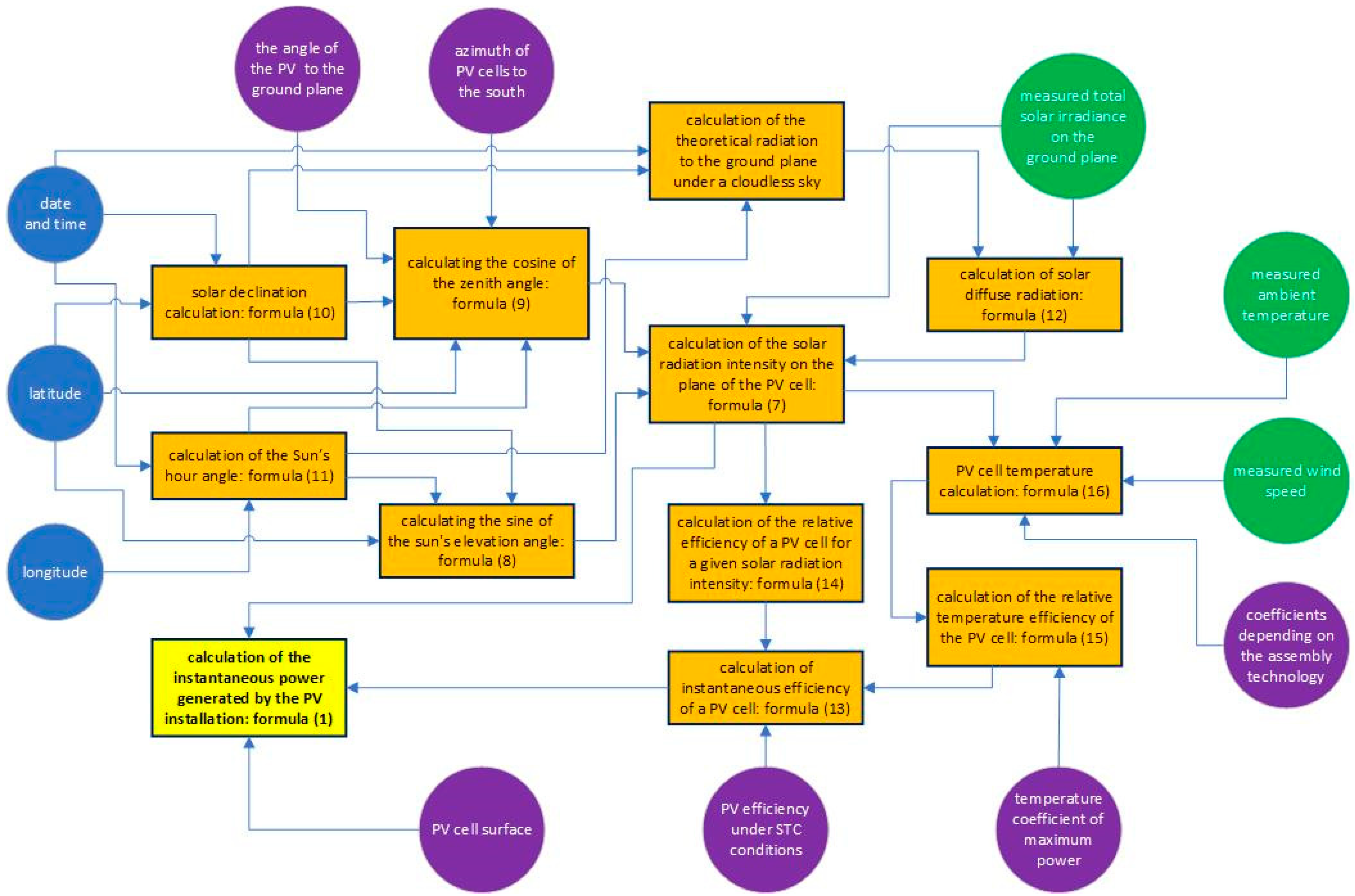
In Section 2, the authors developed a mathematical model for calculating instantaneous total solar irradiance on a PV cell plane. The end result G_PV was obtained using Formula (7). Whereas, in Section 3, the authors developed a mathematical model for instantaneous PV cell efficiency. The end result η_PV was obtained using Formula (13). After substituting the results from Formulas (7) and (13) into Formula (1), we obtained the final instantaneous PV power value. Input data for the aforementioned formulas were, of course, developed using the numerous supplementary formulas discussed in Section 2 and Section 3. The graphical interpretation of the mathematical model was demonstrated using a diagram for calculating PV system instantaneous power in Figure 6.

The input data for the mathematical model in the diagram is presented in circles of different colours, namely, geographical data (blue), instantaneous data values measured by the weather station (green) and PV system technical data (purple). The calculated physical quantity with an indication of the employed formula is presented in rectangles (the calculation of theoretical radiation to the ground plane under a cloudless sky is presented in [50]]). The arrows between the figures represent data flow. The final, expected result of employing the mathematical model in question is calculating the PV system’s instantaneous power for measured meteorological data, such as total solar irradiance, ambient temperature and wind speed.

The mathematical model enables calculating instantaneous power. These calculations are conducted on a regular and cyclic basis, in short time intervals (every 5 min as part of the studies conducted by the authors). In turn, this creates a simulated power waveform for a given PV system in the longer perspective. As indicated in the title of the paper, the presented power waveform simulation model is to be employed for diagnosing PV systems.

The diagnostic method is based on comparing simulated and actual power waveforms. Only the data from the inverter can be used as values of actual PV system power, assuming remote data acquisition. Power determined using Formula (23) was adopted.

$$P_{PV}=I_{PV}·U_{PV},$$

(23)

where P_PV—inverter input power [W], I_PV—inverter input current [A], U_PV—inverter input voltage [A].

As a rule, simulation accuracy will have a significant impact on diagnostic credibility. Error sources were therefore analysed.

One of the sources may be the difference between the calculated and actual diffuse radiation intensity. Significant efforts were made for the calculation Formula (12) to be optimal, as thoroughly discussed in [50], but the spread of diffuse radiation is high due to its variable structure and changing ambient conditions. In addition, the accuracy of calculating the total irradiance on the PV cell surface G_PV is impacted by the assumption that 100% of solar radiation originates from a point light source and that circumsolar glow is not taken into account. Another important error source is the finite accuracy of calculating the temperature of the semi-conductor cell structure t_PV. Section 3 provides the thorough rationale behind the selection of the optimal temperature model. However, there may be differences between the calculated and actual values, depending on technical and atmospheric conditions. The developed PV cell efficiency model, as a function of solar irradiance β_PV, can also be the source of calculation inaccuracies. Furthermore, the model employs the technical parameters of PV cells and systems, such as efficiency under STD conditions β_STD, the maximum power temperature coefficient β_t, system angle of inclination β and azimuth γ. Each of the parameters may constitute a bias source.

However, the source most significantly impacting power calculation accuracy is meteorological data measurement errors. At the same time, errors in measuring ambient temperature and wind speed are of secondary importance. Errors in the measurement of total irradiance on the plane parallel to the Earth’s surface have the greatest impact.

Error sources for a PV system’s power waveform treated as real power waveform were also analysed. The current and voltage values of the inverter input (23) are burdened with measurement errors.

In addition, a comparison of simulated and measured power waveforms is also impacted by measurement time synchronization accuracy and the proximity of meteorological sensors and PV systems.

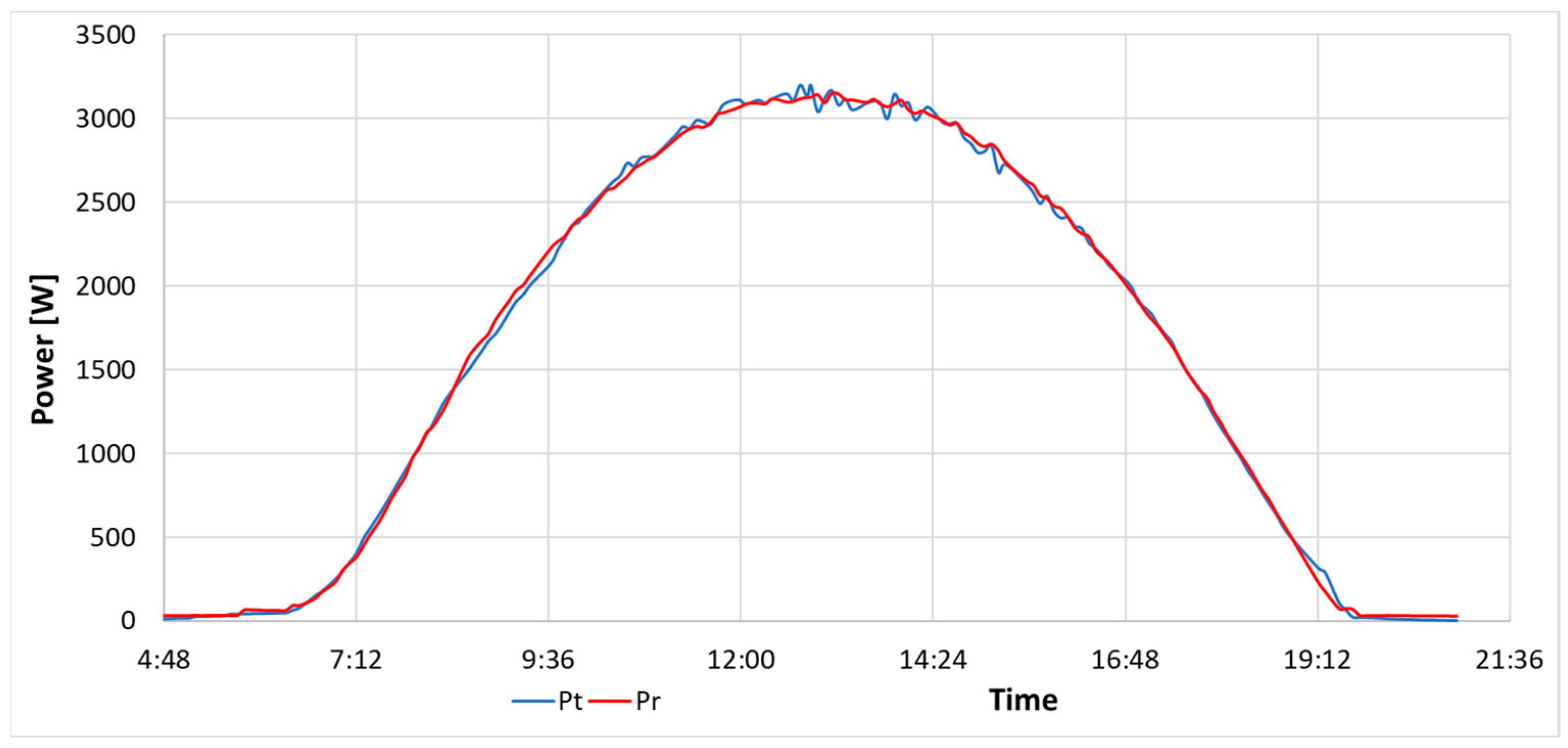
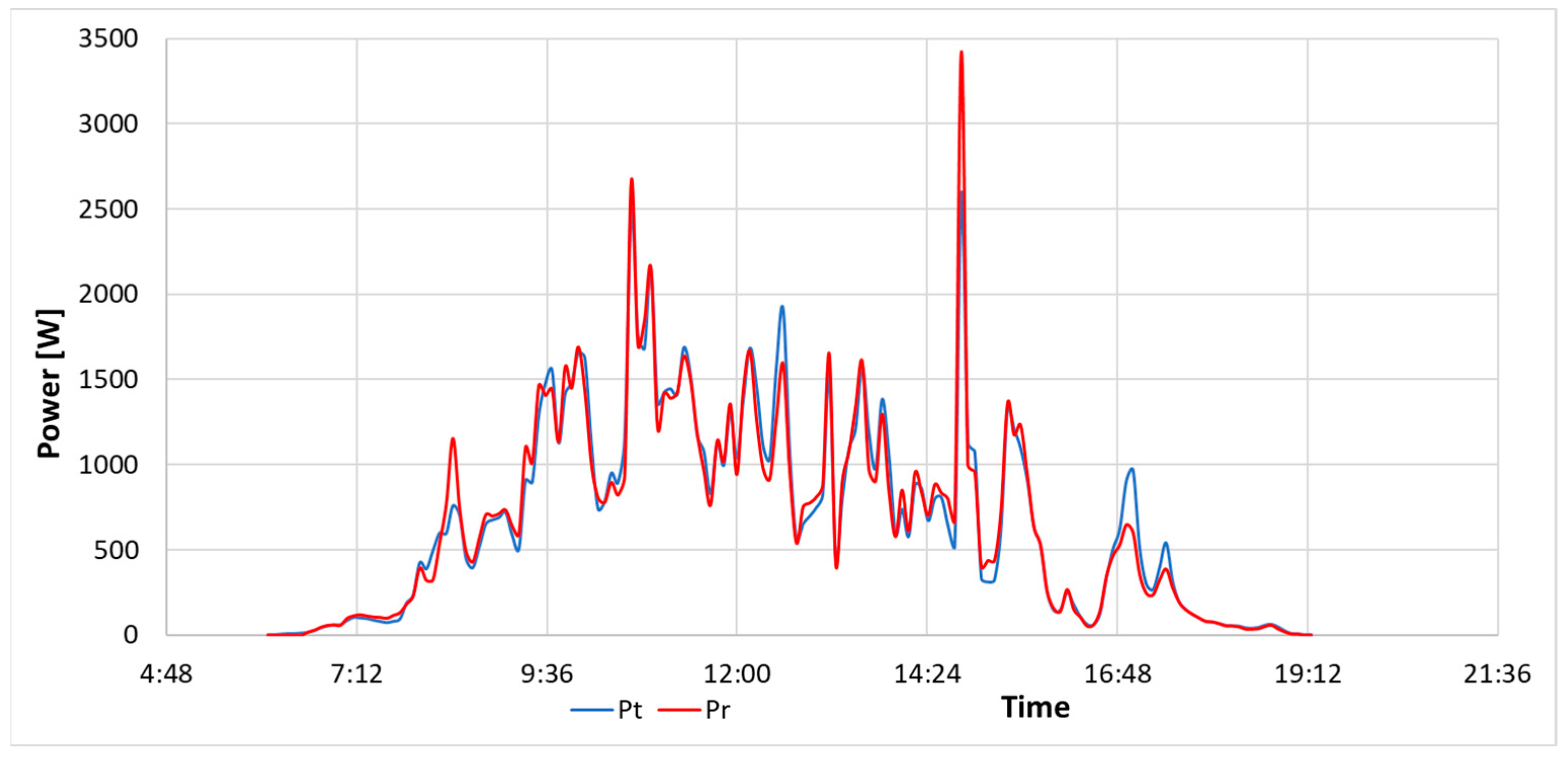
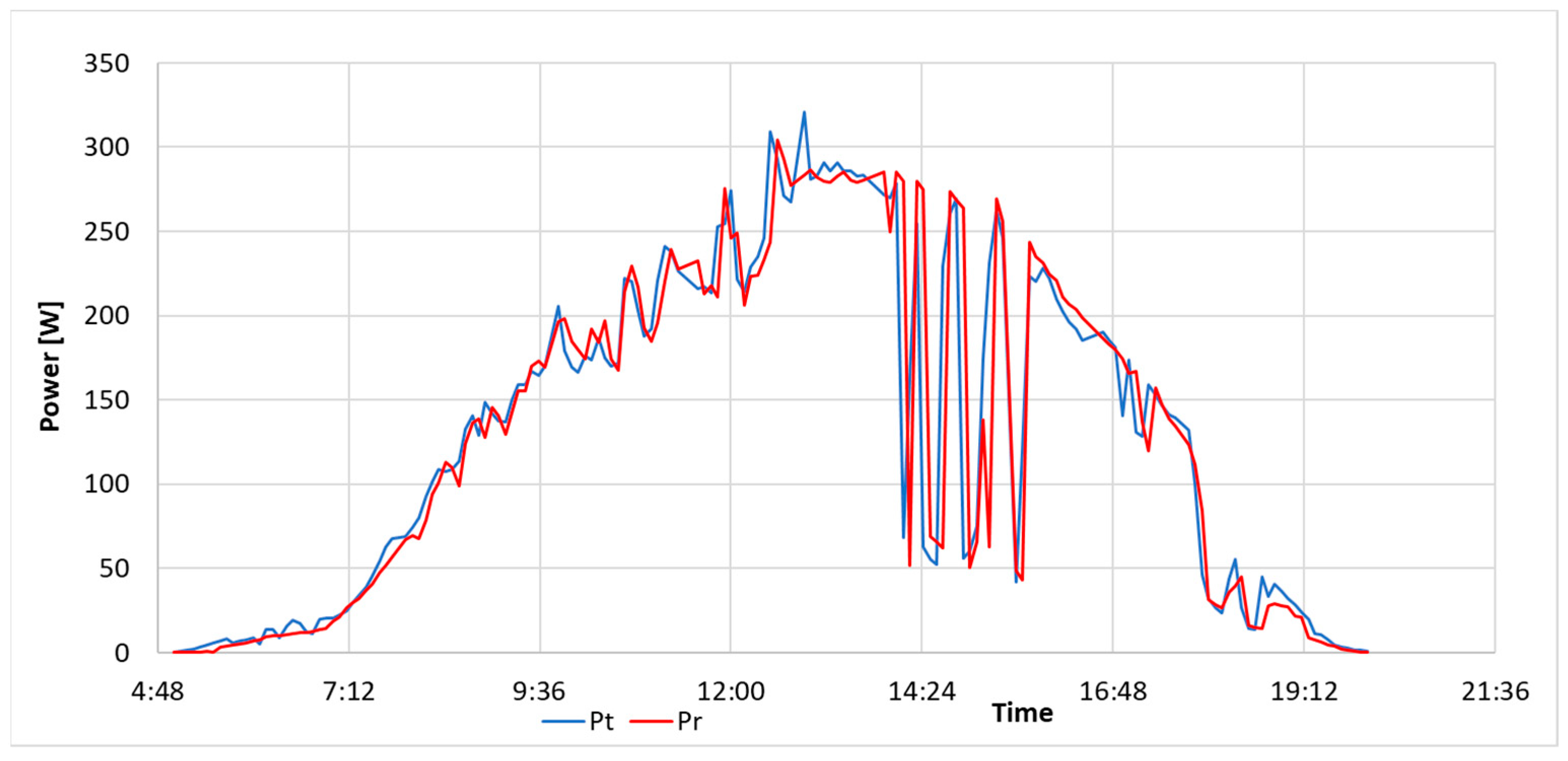
The aforementioned theoretical analysis of a large number of potential error sources became useful when developing and evaluating the mathematical model. However, its practical usefulness is determined by the accuracy of reproducing actual PV system power waveforms. Power waveforms were compared using data from five PV micro-systems under various weather conditions. Figure 7, Figure 8 and Figure 9 show three cases of daily theoretical power waveforms Pt (blue) calculated using the presented mathematical model and the actual power Pr (red). The graphs in Figure 7 and Figure 8 refer to PV system strings and the Pr waveforms are presented based on inverter measurements. The graph in Figure 9 refers to a single cell and the Pr waveform shows recorded data from a power optimizer.

As evident, theoretical and actual power waveforms are very similar, especially under conditions of good insolation (Figure 6). There are sometimes differences in the case of fast-changing insolation conditions, which primarily result from inaccurate measurement data acquisition time synchronization.

The high degree of theoretical and actual power waveform convergence indicates a good simulation model quality, but daily energy yields, calculated using Formula (24), are the most important from the perspective of the research objective.

$$E={\sum }_{i=2}^{i=N}\frac{P_i+P_{i-1}}{2}\left(t_i-t_{i-1}\right),$$

(24)

where E—energy generated by a PV system within a day [kWh], P_i—measured or calculated power for time t_i [kW], P_i−1—measured or calculated power for time t_i−1 [kW], t_i—data measurement time for sample number i [h], t_i−1—data measurement time for sample number i−1 [h].

By substituting the power measured on the inverter or optimizer output to the Formula (23), we obtain the actual energy generated by a PV system within a day E_r. Whereas, when substituting the power calculated using the mathematical model, we obtain the theoretical energy E_t that should be generated by a PV system within a day for actual meteorological data. Daily theoretical and actual energy for waveforms from Figure 7, Figure 8 and Figure 9 are shown in

Table 2. Daily theoretical E_t and actual E_r energy for waveforms from Figure 7, Figure 8 and Figure 9.

PV System Data	Insolation	Date	Et [kWh]	Er [kWh]	Er/Et [%]
string, 11 PV cells, 325 W each	very good	5 June 2022	8.962	8.976	100.15%
string, 10 PV cells, 350 W each	moderate	1 April 2023	26.04	26.10	100.21%
a single PV cell, 340 W power	variables	1 May 2022	1.818	1.811	99.64%

.

The presented cases show very similar values of daily energy acquired within a fit PV system and energy calculated using the simulation model. Therefore, it can be assumed that the discussed mathematical model will be useful for diagnosing malfunctions leading to a PV system energy efficiency deterioration.

5. Application of the Simulation Model to Diagnose PV Systems

Energy efficiency deterioration is a manifestation of numerous PV micro-system malfunctions. This is certainly the outcome of a PV cell failure. It can result from the progressive shading, soiling or ageing of PV cells. Therefore, determining the energy efficiency deteriorations of a string of serially connected cells is very desirable when operating PV systems. However, it is a challenging task when performed on a remote basis for micro-systems without power optimizers or other devices that monitor the parameters of each PV cell. The high fluctuation of meteorological parameters that is inherent to the Central European climate significantly hinders detecting even considerable drops in energy efficiency. Comparable insolation cycles appear in an annual period and may additionally be very diverse. To minimize the influence of cyclicity and fluctuations of weather conditions, the authors suggested employing a standardized energy efficiency coefficient (ξ_PV—hereinafter the interchangeably used SEEC) for PV systems, defined by Formula (25).

$${\xi }_{PV}=\frac{E_r}{E_t}$$

(25)

where ξ_PV—PV system SEEC, E_r—actual energy generated by a PV system over a pre-set period of time [kWh], E_r—theoretical energy calculated using a simulation model for a PV system and actual meteorological parameters over a pre-set period of time [kWh].

Any time period could be used to calculate the coefficient defined by Formula (25), but a period of one day was adopted as optimal, namely, from sunrise to sunset. The diurnal ξ_PV will be further employed for such daily periods.

The procedure for diagnosing PV system unfitness conditions associated with their reduced efficiency was developed using the daily SEEC. To start with, the procedure requires developing a simulation model and data set for a fit system, through:

• entering necessary PV micro-system technical and structural parameters into the simulation model;
• downloading data recorded by the inverter and calculating daily actual energy E_r generated by a fit PV system over a period of at least 20 days;
• downloading data recorded by the weather station (irradiance, temperature, wind speed) for the same time period and calculating daily theoretical energy E_t for the PV system;
• calculating SEEC for at least 20 days;
• determining statistical parameters for the primary SEEC set of a fit system.

With a correctly configured simulation model and the statistical parameters of a set of ξ_PV coefficients for a given PV system in a state of fitness, the diagnostic process will be as follows:

• downloading data recorded by the inverter and calculating daily actual energy E_r generated by a fit PV system over a period of the last several days;
• downloading data recorded by the weather station for the same time period and calculating daily theoretical energy E_t for the PV system;
• calculating SEEC for the studied time period;
• diagnostic inference based on comparing SEEC sets from a current test and an SEEC set from the primary test for a fit system;
• assessing PV system state and diagnosis credibility.

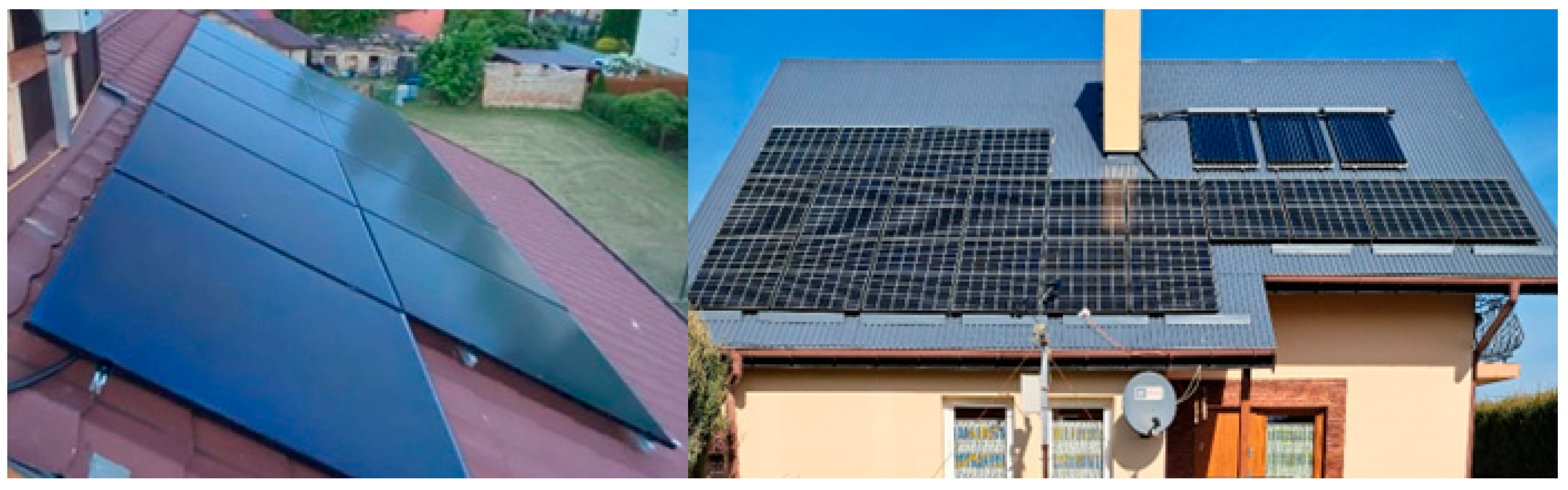
The correct functioning of the assumed diagnostic procedure was verified based on experimental studies involving two photovoltaic micro-systems.

The first studied PV micro-system (I-1) comprised 11 string-connected solar modules with an active area of 1.625 m² each. According to the data of the PV cell manufacturer, the maximum power under STC conditions is 325 W, with an efficiency of 20%, and the maximum power temperature coefficient is—0.36%/°C. PV cells were installed on a building roof with an inclination angle relative to the ground of 26° and an azimuth of 15°. The geographical location of the system was: 52.63, 19.99.

The second PV micro-system (I-2) consisted of two strings, with only one of them used for the analyses as part of this article, since the second one was subject to periodic shading. The studied string comprised 10 modules with an active area of 1.823 m² each. According to the data of the PV cell manufacturer, the maximum power under STC conditions is 370 W, with an efficiency of 20.3%, and the maximum power temperature coefficient is –0.35%/°C. PV cells were installed on a building roof with an inclination angle relative to the ground of 40° and an azimuth of 15°. The geographical location of the system was: 51.34, 21.90.

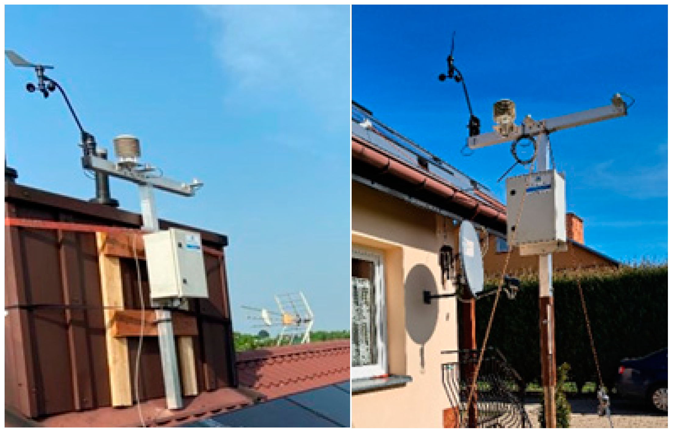
An overview of both systems can be seen in Figure 10.

The inverter data for actual power were downloaded from databases made available as standard by inverter manufacturers. In turn, the weather parameters required by the theoretical power simulation model were measured in direct proximity to the studied systems [63,64], as shown in Figure 11.

The first stage for each micro-system involved conducting tests aimed at determining a sufficiently numerous primary SEEC set for a fit system.

The tests involving the I-1 system lasted for 36 days. The results are presented in

Table 3. Test results for a fit I-1 PV system.

Date	Et [kWh]	Er [kWh]	ξPV = Er/Et [%]
22 May 2022	11.96	10.95	91.58
23 May 2022	18.01	18.54	102.93
24 May 2022	10.56	9.75	92.40
25 May 2022	3.52	3.85	109.32
26 May 2022	14.74	14.61	99.10
27 May 2022	11.51	11.06	96.11
28 May 2022	10.98	11.61	105.69
29 May 2022	10.90	10.51	96.42
30 May 2022	8.84	8.46	95.73
31 May 2022	18.53	19.77	106.69
1 June 2022	13.02	13.18	101.24
2 June 2022	13.68	13.86	101.28
3 June 2022	20.61	20.79	100.92
4 June 2022	18.17	17.62	96.96
5 June 2022	26.04	26.10	100.21
6 June 2022	20.64	19.91	96.47
7 June 2022	15.44	15.78	102.15
8 June 2022	10.63	10.00	94.08
9 June 2022	14.89	14.78	99.24
10 June 2022	8.73	8.85	101.38
11 June 2022	20.50	19.82	96.71
12 June 2022	17.04	16.65	97.67
13 June 2022	3.69	3.63	98.51
14 June 2022	14.14	12.29	86.92
15 June 2022	16.65	15.82	95.03
14 August 2022	15.32	15.44	100.77
15 August 2022	13.08	12.76	97.52
16 August 2022	11.87	11.61	97.81
17 August 2022	9.79	9.87	100.80
18 August 2022	16.19	15.96	98.58
19 August 2022	16.92	16.91	99.93
20 August 2022	9.97	9.51	95.42
21 August 2022	11.06	10.92	98.73
22 August 2022	9.03	9.10	100.78
23 August 2022	9.80	9.42	96.16

.

Standardized energy efficiency coefficient ξ_PV values can be found in the last column of Table 3 and constitute the primary SEEC set for the fit I-1 system. The set of 36 values should be treated as a measurement sample that satisfies the conditions for normal distribution and is sufficient to determine the statistical parameters of sample mean μ₁ = 98.66% and standard deviation σ₁ = 4.14%.

Similar tests were executed for the I-2 PV system, for a period of 35 days. The results are presented in

Table 4. Test results for a fit I-2 PV system.

Date	Et [kWh]	Er [kWh]	ξPV = Er/Et [%]
14 March 2023	13.47	13.04	96.77
16 March 2023	13.61	12.90	94.75
19 March 2023	18.98	18.21	95.92
20 March 2023	12.24	12.83	104.87
21 March 2023	3.79	3.77	99.54
22 March 2023	13.83	13.87	100.34
23 March 2023	8.81	8.56	97.15
24 March 2023	9.10	9.36	102.84
25 March 2023	8.33	7.92	95.06
26 March 2023	11.42	11.11	97.29
27 March 2023	3.34	3.27	97.90
28 March 2023	7.84	7.19	91.64
29 March 2023	26.45	26.21	99.09
30 March 2023	7.40	7.26	98.08
31 March 2023	10.11	9.81	96.98
1 April 2023	8.96	8.98	100.15
2 April 2023	2.95	2.99	101.05
3 April 2023	10.87	10.04	92.41
4 April 2023	11.90	11.43	96.09
5 April 2023	10.48	10.18	97.12
7 April 2023	4.90	4.92	100.29
8 April 2023	16.08	16.51	102.65
9 April 2023	12.47	12.37	99.25
10 April 2023	18.63	19.05	102.27
11 April 2023	19.96	20.20	101.17
12 April 2023	16.58	16.59	100.07
13 April 2023	25.61	26.01	101.54
14 April 2023	18.67	18.77	100.53
15 April 2023	11.74	11.59	98.73
16 April 2023	18.08	18.18	100.56
17 April 2023	6.24	6.18	98.98
18 April 2023	9.84	9.90	100.57
19 April 2023	8.69	8.78	101.08
20 April 2023	19.74	19.67	99.62

.

The last column in Table 4 contains data that constitute a primary set of SEEC for the I-2 fit system. The set of 35 values also satisfies conditions for normal distribution and is sufficient to determine statistical parameters of: sample mean μ₂ = 98.90% and standard deviation σ₂ = 2.81%.

In theory, mean values should amount to 100% for a perfectly configured simulation model, fit PV systems and the absence of measurement sensor biases. However, please note the initially adopted assumption that diagnosis is remotely conducted, with minimum costs and under conditions that can be implemented in actual existing systems. Therefore, the technical and structural parameters provided by the manufacturer and measurement data from an inverter and a simple weather station are employed. The mean value can be particularly impacted by PV cell soiling, the PV cell ageing process, minor overestimation of efficiency under STD conditions by the manufacturer, inverter delay in tracking the MPP (maximum power point) for dynamically variable insolation and measurement sensor biases.

In turn, measurement uncertainty and the associated standard deviation are affected by most of the factors described in Section 3. Bear in mind that the dominant factor is the variability of weather conditions. The measurements involved radiation intensity, temperature and wind speed, with other atmospheric parameters (e.g., particulate matter level, precipitation, pressure) also having a certain impact. In addition, the solar irradiance sensor had slightly different characteristics than PV cells.

Nonetheless, the obtained SEEC sets for the studied PV systems indicate a high potential [58] for diagnosing deterioration of their energy efficiency. This can be seen in the probability density function waveforms shown in Figure 12. Because the mean values of both primary sets are similar, the figures also demonstrate a distribution of a combined primary set for both systems that contains 71 samples and has the following normal distribution parameters: sample mean μ = 98.78% and standard deviation σ = 3.55%.

However, an illustrative graphic interpretation does not constitute sufficient proof, therefore, the authors presented an analytical interpretation. Mean value confidence intervals for a pre-set significance level constitute analysis grounds. The authors adopted a basic significance level of α = 0.01; i.e., a confidence level of 0.99. The confidence intervals for primary sets are shown in

Table 5. Confidence intervals for primary sets at a significance level of α = 0.01.

Installation PV	Sample Mean [%]	Standard Deviation [%]	Confidence Interval [%]
			Minimum	Maximum
I-1	98.66	4.14	96.88	100.4
I-2	98.90	2.81	97.68	100.1
I-1 and I-2	98.78	3.55	97.69	99.87

.

The statistical data for primary sets indicate a possible, highly reliable diagnosis of energy efficiency deterioration of already 2%.

The theoretical analysis of the possible diagnosis of energy efficiency deterioration was verified through experimental tests. The authors simulated a failure of one or two PV cells within a string, by tightly covering them with a material impervious to sunlight. As a result, the covered modules were fully deactivated, and the current flowed through bypass diodes.

Tests involving 17 days for one unfit cell and 7 days for two unfit cells were conducted for the I-1 system. The results are shown in

Table 6. Test results for the I-1 PV system with one unfit module.

Date	Et [kWh]	Er [kWh]	ξPV = Er/Et [%]
17 June 2022	19.19	17.05	88.84
18 June 2022	21.04	17.59	83.63
19 June 2022	24.48	21.24	86.75
20 June 2022	4.64	4.18	90.12
21 June 2022	12.09	10.57	87.43
22 June 2022	24.70	21.67	87.72
26 June 2022	26.09	22.71	87.05
27 June 2022	24.30	21.43	88.20
28 June 2022	18.33	15.74	85.87
29 June 2022	15.38	13.97	90.84
30 June 2022	23.05	20.51	89.01
27 August 2022	12.67	11.32	89.32
28 August 2022	11.88	10.80	90.95
29 August 2022	14.06	13.11	93.18
30 August 2022	5.17	4.51	87.21
31 August 2022	12.75	11.07	86.78
2 September 2022	12.41	11.16	89.87

and

Table 7. Test results for the I-1 PV system with two unfit modules.

Date	Et [kWh]	Er [kWh]	ξPV = Er/Et [%]
23 June 2022	17.88	14.37	80.38
24 June 2022	24.78	19.40	78.29
25 June 2022	26.28	20.26	77.09
3 September 2022	19.23	15.20	79.05
5 September 2022	19.14	15.56	81.28
6 September 2022	20.23	16.10	79.59
7 September 2022	21.11	16.65	78.87

.

The respective statistical parameters are sample mean μ₁₁ = 88.40% and standard deviation σ₁₁ = 2.18%.

The respective statistical parameters are sample mean μ₁₂ = 79.22% and standard deviation σ₁₂ = 1.27%.

Thirteen-day tests for only one unfit cell were conducted for the I-2 system. The results are shown in

Table 8. Test results for the I-2 PV system with one unfit module.

Date	Et [kWh]	Er [kWh]	ξPV = Er/Et [%]
23 April 2023	25.03	23.01	91.91
24 April 2023	21.51	19.98	92.90
26 April 2023	12.25	11.48	93.79
27 April 2023	12.81	11.01	85.94
28 April 2023	17.56	15.49	88.25
29 April 2023	21.81	18.43	84.52
30 April 2023	19.84	16.76	84.49
1 May 2023	27.92	24.15	86.49
2 May 2023	17.63	15.86	89.94
3 May 2023	14.12	13.07	92.60
4 May 2023	27.80	24.29	87.37
5 May 2023	16.60	14.56	87.69
6 May 2023	9.97	8.68	87.03

.

The respective statistical parameters are sample mean μ₂₁ = 88.69% and standard deviation σ₂₁ = 3.09%.

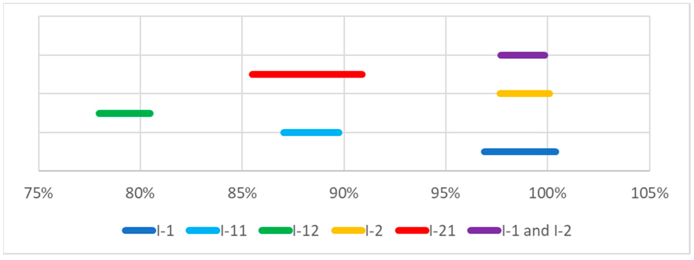
The confidence intervals for SEEC sets with a significance level of 0.01 were determined for systems with one or two unfit PV cells. The confidence intervals are compared in

Table 9. Confidence intervals for primary sets at a significance level of α = 0.01.

Installation PV	Sample Mean [%]	Standard Deviation [%]	Confidence Interval [%]
			Minimum	Maximum
I-1	98.66	4.14	96.88	100.4
I-11	88.40	2.18	87.04	89.76
I-12	79.22	1.27	77.98	80.46
I-2	98.90	2.81	97.68	100.1
I-21	88.69	3.09	86.48	90.9
I-1 and I-2	98.78	3.55	97.69	99.87

and presented in graphic form in Figure 13.

Figure 13 contains confidence intervals for the following cases:

• I-1—PV system No. 1, fit;
• I-11—system No. 1 with one unfit PV cell;
• I-12—system No. 1 with two unfit PV cells;
• I-2—PV system No. 2, fit;
• I-21—system No. 2 with one unfit PV cell;
• I-1 and I-2—combined primary sets for both PV systems.

Based on the data from Table 9 and Figure 13, it can be seen that the confidence levels for systems with unfit PV cells are fully disjointed from confidence intervals for the fit systems. This indicates a possibility of diagnosing a malfunction that involves a failure of one PV cell.

The shown data represent sets with a sample population of at least 11. This is of little significance in the case of primary sets for a fit system, since it is assumed that this will be a one-off test at the initial stage of a system’s operation. Furthermore, in the case of systems permanently fitted with weather stations, the SEEC will be systematically calculated and data from the entire PV system operation period can be employed within the diagnostic process. However, when diagnosing PV systems using mobile weather stations, it is recommended for the test duration to be as short as possible in order to minimize costs. The diagnosis duration expressed in days will be responsible for the sample population.

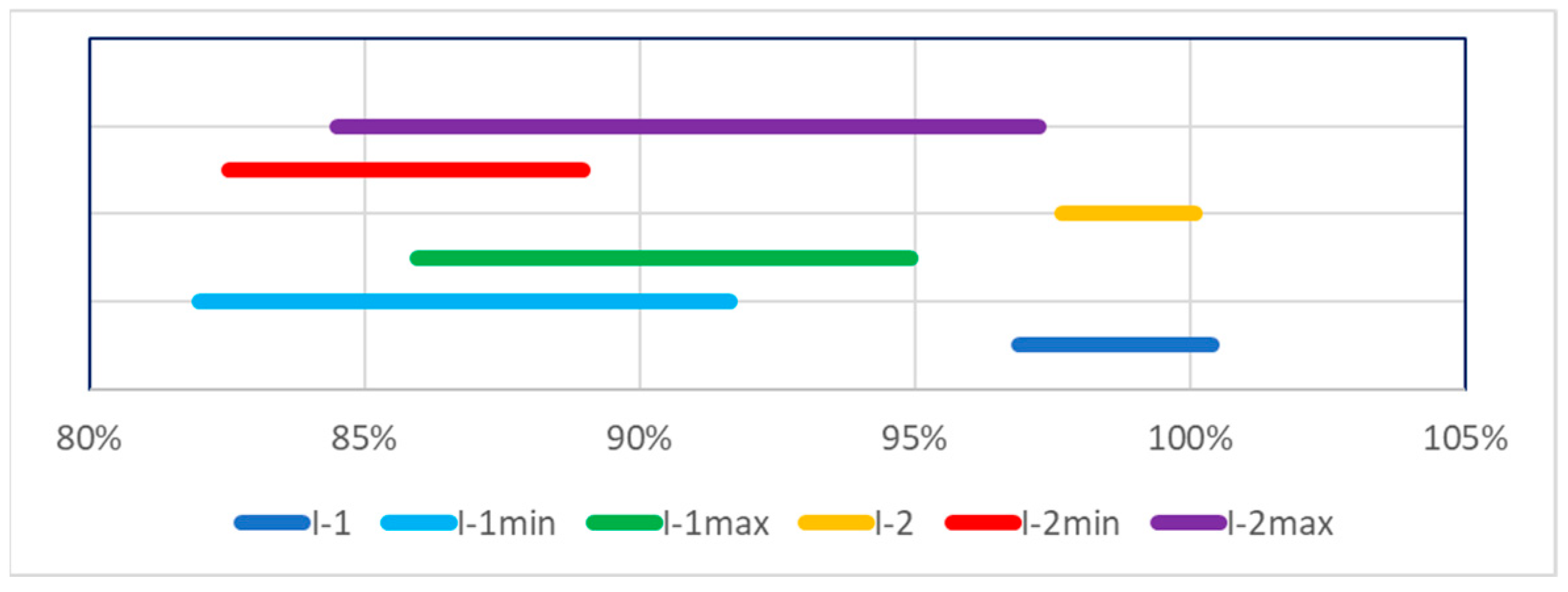
Therefore, the authors analysed data for systems with one unfit PV cell, which are included in Table 6 and Table 8. All possible subsets of three consecutive samples were considered, and confidence intervals with a significance level of 0.01 were determined for them. Extreme cases for both systems are shown in

Table 10. Confidence levels for extreme cases of three-element SEEC subsets.

Installation PV	Sample Mean [%]	Standard Deviation [%]	Confidence Interval [%]
			Minimum	Maximum
I-1	98.66	4.14	96.88	100.40
I-1 min	86.83	3.24	82.01	91.65
I-1 max	90.45	3.01	85.97	94.93
I-2	98.90	2.81	97.68	100.10
I-2 min	85.75	2.16	82.54	88.96
I-2 max	90.88	4.30	84.49	97.27

and Figure 14.

Figure 14 contains confidence intervals for the following cases:

• I-1—PV system No. 1, fit;
• I-1 min—three-element subset of results for system No. 1 with one unfit PV cell, with the lowest initial confidence interval value;
• I-1 max—three-element subset of results for system No. 1 with one unfit PV cell, with the highest final confidence interval value;
• I-2—PV system No. 2, fit;
• I-2 min—three-element subset of results for system No. 2 with one unfit PV cell, with the lowest initial confidence interval value;
• I-1 max—three-element subset of results for system No. 2 with one unfit PV cell, with the highest final confidence interval value.

Based on the data from Table 10 and Figure 14, it can be seen that the confidence intervals for any subset of three consecutive SEEC samples for systems with one unfit PV cell are disjointed from the confidence levels for fit systems. This evidences that even three-day measurements enable a highly credible diagnosis of a malfunction that involves a functional failure of one PV cell.

6. Summary and Conclusions

The article presents an original mathematical model that describes the PV system power waveform based on measured meteorological values, as well as structural and technical data. The high conformity of simulated waveforms with power waveforms recorded for three actual PV systems differing in structural parameters and geographical location was also demonstrated.

A standardized energy efficiency coefficient was developed based on the mathematical model. Then, the daily (diurnal) SEEC was utilized as a diagnostic parameter for diagnosing failures of individual cells in the PV system or other failures leading to efficiency deterioration. To verify the diagnostic capabilities based on SEEC, the authors conducted tests involving two micro-systems with different parameters and geographical locations.

The conducted analysis of measurement results and conducted calculations enables drawing the following conclusions:

• It was confirmed that the functional mathematical model of a photovoltaic module generates results consistent with the energy yield results obtained from an actual PV system. This conformity is statistically confirmed for a significance level of α = 0.01.
• The SEEC value, which is the quotient of actually generated energy and energy calculated based on the generation process simulation model, taking into account environmental and weather conditions, is diagnostically sensitive. This means that this value can be treated as a diagnostic signal that carries information on the functional state of a PV system.
• It was confirmed that SEEC diagnostic signal value sets exhibit statistically significant differences, depending on the PV system functional state.
• The described experiment involved testing a PV system in a state of full fitness and in two states of incomplete functional fitness. States of incomplete fitness involved isolating light falling on one or two PV cells. This physically means simulating a failure. The authors identified a sensitivity of the proposed diagnostic signal value to such malfunctions. It is sufficient from the perspective of a system user and diagnostics specialist.
• The test significance level employed in the analysis above (α = 0.01) means that the maximum error of a statement that the compared mean value confidence levels do not differ (when in reality they are significantly different), at 1%.
• The conducted tests studying the sensitivity of SEEC values to a change in PV system state as a function of the set population indicate that a state change can be credibly already inferred with a set of three readings (Figure 14).

The presented diagnostic procedure, being implemented in the form of a computer app, can be employed in PV micro-system monitoring centres. The occurrence of reduced PV system energy efficiency can be identified with a high level of credibility based on mean SEEC values calculated for at least three-day remote measurements. It will enable shortening the time from the occurrence of a PV malfunction until its detection, and hence, limiting energy losses. The application of the described SEEC determination model and the proposed diagnostic procedure enables changing the PV system maintenance type—from servicing by operation time to servicing by current condition [65].

The diagnosis method described in the article, which is based on the diurnal SEEC, is characterized by its remote data acquisition ability, low equipment cost (with only a basis weather station required), the relatively short time needed to determine a diagnosis and high reliability. Diagnosis initiation requires introducing detailed technical and structural parameters, but it is also possible to automatically download them from the management system related to a given PV system.

Referring to the methods based on other symptoms, one can infer that:

• methods based on thermal imaging require relatively expensive cameras and do not offer the possibility to assess thermal effectiveness, but enable diagnosing other defect types; e.g., hot spots;
• methods based on artificial intelligence usually require a relatively long learning time but the diagnosis credibility in the case of high weather variability is problematic;
• methods utilizing statistical analysis may have reduced diagnosis credibility in the case of high weather variability;
• methods based on comparing adjacent chains exhibit low effectiveness in diagnosing micro-systems due to a frequent absence of close proximity to other PV systems.

Therefore, the SEEC-based diagnosis proposed by the authors comes with great potential application for remote PV micro-system condition monitoring.