Abstract
Efficient train driving plays a vital role in reducing the overall energy consumption in the railway sector. An energy minimising control strategy can be computed using the framework given by optimal control theory; in particular, the Pontryagin maximum principle can be used. Our optimisation approach is based on an algorithm presented by Khmelnitsky that considers electric trains equipped with regenerative braking. A derivation of Khmelnitsky’s theory from a more general formulation of the maximum principle is given in this article, and a complete list of switching cases between different driving regimes is included that is essential for practical application. A number of numerical examples are added to visualise the various switching cases. Energy consumption data from real-life operation of passenger trains are compared to the calculated energy minimum. In the presented study, the optimised strategy was able to save 37 percent of the average energy demand of the train in operation. The sensitivity of the energy consumption to deviations of the train speed from the optimum speed profile is studied in an example. Another example illustrates that the efficiency of regenerative braking has an effect on the optimum speed profile.
1. Introduction
Energy-efficient driving strategies have been shown to substantially lower the total energy consumption of railway trains. With an increased demand for energy saving technologies, numerous research studies have been devoted to this subject in recent years, showing that, in many cases, an average energy saving from 15 to 30% could be achieved by assisted driving [1,2,3,4,5,6,7,8]. A comprehensive review on energy-efficient train control, commonly abbreviated as EETC, is given by Scheepmaker, Goverde, and Kroon [9]. The majority of the mathematical models that have been developed to calculate energy-minimised driving are based on Pontryagin’s maximum principle (PMP), a fundamental theorem of optimal control theory. The maximum principle was formulated in 1961 by Pontryagin, Boltyanskii, Gamkrelidze, and Mishchenko [10,11]. The first application of Pontryagin’s maximum principle to the operation of trains dates back to Japanese research in 1968 (Ichikawa [12]). The model of Ichikawa was restricted to a flat track and linear train resistance depending on speed. Another early contribution is due to Strobel, Horn, and Kosemund [1]. They considered a non-constant altitude and found that the optimal solution is always in one of the drive regimes, namely full traction, partial traction with constant speed, coasting, partial braking with constant speed, and full braking. Based on their model, they set up a first driver advisory system for the Berlin S-Bahn (suburban trains).
Since those pioneering research on this topic, models have gained complexity. Important developments have been: (1) the application to variable altitude and variable speed limit, (2) the inclusion of regenerative braking in electric locomotives or motor coaches, (3) improved modelling for train resistance, tractive, and brake force depending on speed, (4) the energy minimisation with non-zero speed boundary conditions, (5) advanced modelling of efficiency as dependent on speed, tractive, and brake force, (6) the modelling of discrete throttle settings for diesel engines instead of continuous traction, and (7) multiple-train problems.
Regarding the second aspect, some (especially the earlier) authors are dealing only with the mechanical braking of trains. When regenerative braking is considered, most authors base their energy-efficient driving strategy on the exclusive use of the regenerative brake. A few recent contributions cover the combined application of the mechanical and regenerative brake in their optimisation strategy.
We proceed with some important developments for purely mechanical braking. Starting from the Ph.D. thesis of Milroy [13] in 1980, a research team at the University of South Australia introduced the system Metromiser (Howlett and Pudney [2]). The system covered both timetable planning and driver advisory. Metromiser was restricted to constant track gradients during both coasting and braking. The system was first applied on trains in Adelaide (Australia) in 1984, followed by Toronto (Canada), Melbourne (Australia), and Brisbane (Australia). Howlett, Milroy, and Pudney [14] were the first to assume a variable speed limit, but only for the special case of discrete traction control. In 2003, Liu and Golovitcher [15] presented a method covering variable altitude, variable speed limit, continuous traction control, and quadratic train resistance dependence on speed. Except being bound to purely mechanical braking, this algorithm is therefore quite general with respect to the other assumptions. The article contains a complete description of switching between the possible drive regimes. In 2013, Albrecht, Howlett, Pudney, and Vu [16] introduced the driver advisory system Energymiser that was applied by the French railway SNCF on TGV high-speed trains. They proved the uniqueness of the energy optimum being derived. A multi-objective algorithm combining energy minimisation and the punctuality of trains was developed by Aradi, Becsi, and Gaspar [6].
Regenerative braking was first considered in 1985 by Asnis, Dmitruk, and Osmolovskii [17] in the context of train energy minimisation. They assumed a constant altitude and speed limit in their model. Franke, Terwiesch, and Meyer [3] introduced an energy optimisation algorithm for variable altitude, variable speed limit, and purely regenerative braking that was restricted to piecewise constant traction and brake force. They suggested a discrete dynamic programming (DDP) method as a solution. In 2000, Khmelnitsky [18] developed a model that covered variable altitude, variable speed limit, continuous traction control, arbitrary maximum tractive and brake force depending on speed, quadratic train resistance with respect to speed, and exclusively regenerative braking. Regarding these features, they provide broadly applicable approaches with few restrictions. Due to these advantages, the algorithm of Khmelnitsky was chosen as the basis for our research. In a recent article by Ying et al. [19], the EETC problem solved by Khmelnitsky was revisited, with a special focus on solutions reaching the speed limit. The paper of Ying et al. [19] can be especially recommended for its comprehensive illustration of the large variety of cases that can arise during the construction of the optimum solution. The EETC problem with prescribed non-zero speed boundary conditions was solved by Ying et al. [20].
There are relatively few research contributions dealing with the EETC problem using combined mechanical and regenerative braking. Baranov, Meleshin, and Chin’ [21] were the first considering this topic, but an algorithm to solve the problem was left as an open question in their article. Lu et al. [22] studied combined mechanical and regenerative braking, but excluded both variable speed limit and variable track gradients. Zhou et al. [23] studied the synchronisation of accelerating and braking trains, considering both kinds of braking, but again did not include the variable speed limit. Fernández-Rodríguez et al. [24] combined both brake systems in a multi-objective optimisation method, but did not derive a rigorous energy minimum. In the paper of Scheepmaker and Goverde [25], the optimisation problem with combined mechanical and regenerative braking was solved for the first time under general assumptions, i.e., with a speed dependent tractive and brake effort, variable speed limit, and variable altitude. Scheepmaker and Goverde used the Gauss–Radau pseudospectral method implemented in GPOPS [26] to solve the optimal control problem.
Several authors considered advanced efficiency modelling, in particular efficiency depending on speed, tractive, and brake force. This assumption is more realistic but substantially complicates the approach. Su, Tang, and Li [27], Zhu et al. [28], and Su et al. [29] modelled traction efficiency depending on traction force and speed; they apply the energy-distribution-based method (EDBM) to solve the problem. Research on advanced efficiency modelling was also carried out by Franke, Terwiesch, and Meyer [3], Ghaviha et al. [30], Kouzoupis et al. [31], and Feng, Huang, and Lu [32]. Discrete traction control, which is relevant for diesel engines with discrete throttle settings, was considered by Howlett, Milroy, and Pudney [14]; Cao et al. [33]; and Zhang, Cao, and Su [34]. Multiple train problems were often been studied with a focus on timetable design in order to synchronise accelerating and braking trains for the best distribution of regenerative energy. See, for example, Zhou et al. [23] for research on this topic. More references can be found in Scheepmaker and Goverde [25]. Szkopiński and Kochan [35] studied energy-efficient train driving when approaching a train on the track ahead. Su et al. [36] introduced a stabilisation strategy that avoids frequent switching between traction and braking on sections where the energy optimum would actually require a coasting regime. An algorithm for energy-efficient train driving with multiple time targets that can be used for timetable design was developed by Fernández-Rodríguez et al. [37].
Apart from the many research contributions based on an application of Pontryagin’s maximum principle, a variety of other methods exist to solve the EETC problem. In particular, the so-called direct methods have recently gained attention. They are characterised by the fact that the problem is first discretised, usually by dividing the track length into smaller intervals. The resulting nonlinear programming (NLP) problem is then solved by nonlinear programming methods as, for example, the pseudospectral one. Wang et al. [38] were the first to apply the pseudospectral method to an EETC problem. Scheepmaker and Goverde [25] also utilised a pseudospectral approach. Direct methods have the advantage of being very flexible with respect to the problem under consideration. In addition, optimal control solvers such as DIDO (Direct and Indirect Dynamic Optimization) [39,40,41], PSOPT [42,43], or GPOPS-II (General Pseudospectral Optimal Control Software) [26,44] are readily available. The implementation is much easier than a solution of the problem along the lines of Pontryagin’s maximum principle. On the other hand, the pseudospectral method often shows an inaccurate oscillatory behaviour of solutions, and it tends to be time consuming [31]. Recently, Kouzoupis et al. [31] were able to reduce the computing time of a direct method using multiple shooting.
Based on the above-mentioned approach of Khmelnitsky [18], a programme called Leda (low energy driver advisory) was developed at Fraunhofer Institute for Factory Operation and Automation (IFF), Magdeburg, Germany. The code is written in MATLAB and currently features energy minimisation with exclusively regenerative braking, except for the fastest train motion in the case of tight timetables where additional mechanical braking is considered. The choice of Khmelnitsky’s method was mainly motivated by superior accuracy at an acceptable computing time. An extension of the code to fully include mechanical braking into the optimisation is subject to further development, as well as non-zero speed boundary conditions and smooth switching from fast to energy-efficient driving in the case of a train delay. The code was tested offline in numerous cases based on real railway tracks and timetables, and the computing time was substantially reduced by code optimisation. A couple of tests with driver advisory in a real-life operation demonstrated energy savings of about 20% compared to the average of unassisted runs.
The main motivations of this article can be summarised in the following way:
- It is intended to show a direct derivation of Khmelnitsky’s theory from a more general formulation of Pontryagin’s maximum principle given by Hartl, Sethi, and Vickson [45]. By seeing Khmelnitsky’s theory in this general framework, extensions to other conditions could be elaborated.
- Our aim is to provide a comprehensive illustration of the behaviour of the method of Khmelnitsky using a couple of numerical examples. We felt that this very useful method would strongly benefit from some illustrative examples that show the behaviour of the trajectory field including kink points as well as the large variety of switching cases from one driving regime to another. We, therefore, put a strong focus on the examples in Section 2.4 and Section 2.5, in which most of the possible switching cases can be studied in detail.
- Another aim of the article is to estimate the energetic potential of an optimal driving strategy by comparing the energy optimum to energy consumption in a real-life train operation. As a result of a study of 100 train runs on a railway line in Germany, the optimal strategy consumed only 63% of the average energy demand of the unassisted runs in a real operation.
- The sensitivity to deviations from the optimum speed profile was studied. This will always be of practical relevance, since in a real application the train driver will manually try to follow the suggestions of an advisory system and therefore will never exactly meet the optimum speed profile.
This article is structured in the following way: In Section 2.1, the model of the train motion is introduced. Section 2.2 is devoted to the Pontryagin maximum principle that provides a couple of necessary conditions the energy minimising solution has to fulfil. In Section 2.3, the maximum principle is applied to the specific minimum energy problem for train motion. This leads to the observation that only four driving regimes, full traction, constant speed, coasting, and full regenerative braking, are feasible for an energy-minimising motion. The regime constant speed can be driven only at two specific velocities or at the speed limit. Section 2.4 and Section 2.5 describe the algorithm of Khmelnitsky [18] for the construction of the minimum energy solution. A complete list of switching cases is given and explained in Section 2.4, and four numerical examples are introduced to illustrate those cases. Some directions are given that lead to a substantial reduction of computing time. Section 3 is devoted to the results. It contains the comparison of the optimum strategy to a real-life train operation in Section 3.1, the sensitivity to deviations from the speed optimum in Section 3.2, and finally a study that shows a slight effect of the regenerative brake efficiency on the optimum speed.
2. Materials and Methods
2.1. Model of Train Motion
The equation of motion of a train with an electric engine and both regenerative and mechanical brakes can be given by
where is tractive force, is the force applied by the regenerative brake, is the force of the mechanical brake, is air drag, is rolling friction, is the downhill slope force, is a coefficient representing rotating masses, m is the mass, and a is the acceleration of the train. This is Newton’s second law of motion with the extension of rotating masses, for example, the wheels of the train, are accounted for by a factor . A model of this type is commonly used for train motion, see, for example, the review article of Scheepmaker, Goverde, and Kroon [9] or the textbook of Ihme [46]. According to Ihme [46], for passenger trains, depending on their length, where longer trains will generally have smaller values of .
The tractive force is limited by both engine power and rail friction (adhesion). According to Fassbinder [47],
where is the mechanical engine power used for traction, v is the velocity of the train, is the adhesion coefficient, g is gravity, and is the mass of the locomotive. The adhesion coefficient was obtained experimentally in 1943 by Curtius and Kniffler [48], see, e.g., Schlecht [49], leading to the empirical relation
The adhesion coefficient attains a maximum value of 0.331 when .
The regenerative brake force is, as the tractive force, restricted by engine power and rail adhesion. However, it must be further limited to avoid a derailing of coaches behind the braking locomotive. Thus, for the regenerative brake force there holds
where is the mechanical engine power for regenerative braking, and is the additional limit to avoid derailing. In general, will hold. According to [50], the limit force was recently enlarged in Germany from 150 kN to 240 kN, a value that is also considered in Scheepmaker and Goverde [25].
The first term in the minimum in (2) is the engine power limit of traction force, and the second term is the rail friction limit. Likewise, the first term in the minimum in (4) is the engine power limit of the brake force. If holds, then both engine power limits are equal. The maximum forces and are shown in Figure 1.
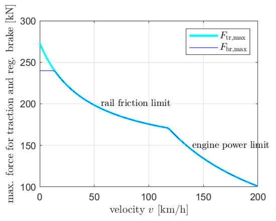
Figure 1.
Maximum force for traction and regenerative brake for an electric locomotive with mass and .
Remark 1.
The correlation (3) for the adhesion coefficient was obtained experimentally under dry conditions. On wet rails, adhesion can be considered to be about 30% less [49]. The roughness of the rail and wheel, as well as the wheel diameter, will have an influence on adhesion, but this was not studied by Curtius and Kniffler [48]. Strictly speaking, the rail friction limit would be , where ϕ is the slope angle of the track. However, even for extremely steep railway tracks, the value of would be very close to one, and the factor can therefore be neglected.
Remark 2.
In practical operation, the regenerative braking of trains is not possible when the speed is too small, meaning that for a final halt, the mechanical brake always has to be applied. This was pointed out by Scheepmaker and Goverde [25], who have estimated a minimum speed of 8 km/h for the application of regenerative braking based on data from Netherlands Railways. However, since kinetic energy below 8 km/h is relatively low, we have neglected this consideration in our model.
When a train brakes, using the regenerative brake is clearly advantageous with respect to saving energy. However, the force of the regenerative brake is limited and, especially for long freight trains, much weaker than the force of the mechanical brake. This is due to the fact that regenerative braking applies only to the wheels of the locomotive, while the mechanical brake acts on every wheel of the train. If the time required by the timetable is too short for a certain distance, purely regenerative braking might not be sufficient. However, as Scheepmaker and Goverde [25] have proven by means of optimal control theory, the mechanical brake is always ‘second choice’ in an energy-minimising solution. This means that mechanical braking is only applied when regenerative braking is operating at maximum force, i.e., when holds. In the optimisation method presented here, the mechanical brake is not incorporated into the theory and will only be considered in the calculation of the fastest possible motion. This will be explained in more detail in the following sections.
The mechanical work applied for traction is given by
where s is track length and t is time. The electric energy required for traction is
The efficiency of electric locomotives is usually given in a range from 83 to 87 percent [25,47,51]. Within this paper, we will use an intermediate value of . Likewise, the mechanical work applied for regenerative braking is
and the electric energy returned will be
We use a braking efficiency according to Fassbinder [47]. The difference is called the net energy, which should be minimised.
In a real operation, additional energy will be required that is not directly related to traction or brake, including energy for air compression, air conditioning, lighting and so on. However, since this additional energy is mainly a function of time, it cannot be reduced by a driving strategy when the total time is constant as given by the train’s timetable. Therefore, the additional energy does not enter the net energy minimisation problem and can be excluded here.
For air drag, Ihme [46] recommends the so-called Hanover Formula that goes back to Voß, Gackenholz, and Wiebels [52]. It takes the form
with air density . In this formula, is not the cross-sectional area of the train, but a reference area of . The air drag coefficient is calculated according to
n being the number of coaches. Ihme [46] provides the values , , , as appropriate for Intercity coaches.
The rolling friction can be modelled by with according to Ihme [46]. The downhill slope force is given by
where z is the altitude of the track.
Remark 3.
The models for the air drag and rolling friction that are used here are simplified relations taken from the literature. In particular, the air drag model considered here can be seen as a rather rough estimate since it does not consider the current wind conditions, which will be difficult to model but might have a significant effect. Some authors (as, for example, Scheepmaker and Goverde [25]) use an overall train resistance equation that was obtained experimentally based on a particular train. If reliable data are available for the specific train under consideration, train resistance modelling based on such data could be considered as a more accurate alternative.
2.2. The Maximum Principle
The problem of minimising the net energy of a scheduled train can be formulated as an optimal control problem, as it was proposed by Khmelnitsky [18], who also presented an algorithm to obtain the unique net energy minimum. The algorithm of Khmelnitsky is essentially based on the maximum principle of optimal control theory that was developed by Pontryagin, Boltyanskii, Gamkrelidze, and Mishchenko [10,11]. A variety of formulations of the maximum principle can be found in Hartl, Sethi, and Vickson [45]. While some of the results of the maximum principle for the particular problem of a minimum energy train ride are already given in Khmelnitsky’s paper [18], a direct derivation from the more general formulation of the maximum principle as presented in Hartl, Sethi, and Vickson [45] is not included in Khmelnitsky. We are, therefore, going to show this derivation here. In Section 2.2, the maximum principle is presented, based on the ‘Informal Theorem 4.1’ in [45]. The subsequent Section 2.3 contains the application to the train problem. Equipped with this general framework, extensions of the theory (for example, the inclusion of the mechanical brake) are possible.
We consider the following problem: Let s be the track length coordinate between two stations at and . The motion of the train is described by the time it takes for the train to move from the first station to position s. We assume and a fixed duration given by the timetable. The velocity v of the train is restricted by a piecewise constant function that accounts for speed limits on the track. Tractive and regenerative brake force, and , are limited according to (2) and (4), respectively. The optimisation problem is to find a motion, i.e., a function , that minimises the net energy .
We introduce some notation, closely following Khmelnitsky [18]. Let be the kinetic energy of the train. Dividing by leads to a specific kinetic energy
limited by speed restrictions: . Likewise, a specific potential energy is defined by
A total specific mechanical energy is then given by . In the same way, specific forces are defined as
A total recuperation efficiency is given by . The aim of minimising the net energy is equal to maximising
With this notation, the optimisation problem can be written in the following canonical form:
- State vector ;
- Control vector ;
- State differential equations;
- State boundary conditions;
- Maximum;
- State constraint ;
- Control constraints and .
Remark 4.
Remark 5.
Further constraints could be added here, especially and . However, will always hold for the energetic optimum solution inside the interval . The condition follows from (21)–(23). Therefore, conditions and need not be set explicitly as a constraint. The simultaneous traction and brake, i.e., and for the same s, is also not explicitly prevented by a constraint since such a solution will surely not be energetically optimal.
Remark 6.
In Equation (20), we have excluded mechanical braking. This means that, in accordance with Khmelnitsky [18], we formulate the optimisation problem only for purely regenerative braking. An extension of the presented theory to the case with a simultaneous application of both regenerative and mechanical brake is possible in a straightforward manner, and is, in a slightly different formulation, given by Scheepmaker and Goverde [25].
Introducing the notation
we have an optimisation problem of the form given in Hartl, Sethi, and Vickson [45]:
In Hartl, Sethi, and Vickson [45], the problem is formulated with a time t being the independent variable instead of s. This is due to the fact that many practical optimisation problems are formulated in a time-dependent way. In our case, however, the position-dependent formulation has some advantages, especially since the speed restriction also depends on position, not on time.
The function
with Lagrange multipliers is called the Hamiltonian of problem (31)–(34). (Here and in the following, means the transposed of a column vector, i.e., is the scalar product of vectors and .) The Lagrange multipliers are also called the costates of the problem. In order to agree with the notation of Khmelnitsky [18], we denote the costates according to
Furthermore, the Lagrangian is introduced by
where and are also called Lagrange multipliers. The Lagrange multipliers , and are continuous functions in s, except for positions where .
The ‘Informal Theorem 4.1’ of Hartl, Sethi, and Vickson [45] states the following necessary conditions for to be a solution of the optimisation problem (31)–(34):
- The control vector maximises the Hamiltonian H pointwise for any , i.e.,is fulfilled. (Here, the subscript ‘opt’ corresponds to the optimal solution.)
- There holds
- The costate equationis satisfied.
- Let be the components of vector , and be the components of vector . There holdsfor all i and all . This is called complementary slackness in Khmelnitsky [18].
- Another complementary slackness condition,holds for all .
- The following jump condition is satisfied: At every point where is discontinuous, there exists a number withHere, the argument corresponds to the left-hand limit, and to the right-hand limit at . The vector Equation (43) is meant to be component-wise.
The Hamiltonian maximisation condition (38) is called the Pontryagin Maximum Principle, and Equations (39)–(42) are referred to as the Karush–Kuhn–Tucker (KKT) conditions [53,54]. In Hartl, Sethi, and Vickson [45], the maximum principle is presented also for the case of multiple state constraints, i.e., when h is extended to a vector. The maximum principle does not, as we shall see, tell the solution to the energy minimisation problem directly, but it provides essential information such that a construction of the solution becomes possible in an iterative trial-and-error process.
2.3. Application of the Maximum Principle to the Energy Minimisation Problem
From the costate Equation (40), it follows for the second component of
since L does not depend explicitly on t. Equation (43) provides, again for the second vector component,
Thus, the Lagrange multiplier is a constant. Equation (39) results in
From the costate Equation (40), first component, we have
When travelling below the speed limit, i.e., , then holds due to (42). (In Khmelnitsky’s notation, and are called and , respectively.) We now apply a case distinction to the multiplier , and evaluate , , and the using the conditions (38), (41), (48), (49), and the continuity of the multipliers. The results are given in Table 1.

Table 1.
Case distinction for . ‘cont.’ means that the continuity of the Lagrange multipliers was exploited. The corresponding value is only valid in the interior of the state domain, i.e., when .
From the values given in Table 1 it follows that, in the interior of the state domain, and can be directly expressed in terms of :
The cases indicated in Table 1 are the only driving modi that are possible for the optimum solution of the problem. This means that the interval can be completely segmented into subintervals with , where every subinterval corresponds to one of the drive modi, namely full traction, partial traction, coasting, partial regenerative brake, and full regenerative brake. The cases full traction, coasting, and full regenerative brake are regular in the sense that the control variables and are both defined, and therefore the equation of motion is completely provided by the underlying physics. On the contrary, the modi partial traction and partial brake are singular, meaning that here only one control variable is defined. Therefore, they need some additional consideration. We will distinguish the following four cases:
Case 1: Partial traction below speed limit. Let be an interval of partial traction in the interior of the state domain, i.e., an interval where and hold. It follows that on this interval; see Table 1. The costate Equation (50) reduces to
with being a known and monotonically increasing function in K. Moreover, the function value is strictly positive for . Since is constant, we have
where stands for the inverse function of R. This means that, for the optimal solution, partial traction in the interior of the state domain is only possible at a constant speed with . From Equation (54) it follows that must hold.
Case 2: Partial regenerative brake below speed limit. Likewise, if is an interval of partial regenerative brake in the interior of the state domain, then and will hold, and the costate equation now reads
Since is constant,
holds, meaning that partial regenerative brake in the interior of the state domain is only possible at a constant speed with . (In Khmelnitsky [18], the constants and are called and , respectively.)
Case 3: Partial traction on the speed limit. Let be an open interval of partial traction on the speed limit. Then, for . Both and are unknown, but the equation of motion is entirely determined by the speed limit with and . Since is piecewise constant, and v can not be discontinuous, v, , K, and must be constant in the interval .
Case 4: Partial regenerative brake on the speed limit. Likewise, if is an open interval of partial regenerative brake on the speed limit, then for . Both and are unknown in this case, but the equation of motion is again entirely determined by the speed limit with and . Both and must be constant on , using the same argument as in Case 3.
The location of the sub-intervals corresponding to the drive modi full traction, partial traction, coasting, and partial regenerative brake, and full regenerative brake is not defined a priori. The intervals will be derived in the algorithm of Khmelnitsky, a process that is shown in the following Section 2.4 and Section 2.5. The process starts with the definition of intervals where constant speed could possibly be driven and proceeds with trials to link these intervals by regular motion trajectories. Finally, if a complete link from the departure point to the arrival point exists that consists of periods with regular motion and admissible constant speed sections, and if this link meets the prescribed total time, then the unique optimal solution is found.
Remark 7.
In recent literature (not in Khmelnitsky), the constant speed driving regimes are often called cruising.
2.4. The Algorithm of Khmelnitsky for Fixed
In this section, we describe the algorithm of finding a solution to the optimisation problem under the assumption that the Lagrange multiplier is a given number. Then, and are defined according to (54) and (56), respectively. Following Khmelnitsky [18], we define intervals with possible constant speed that correspond to the four cases studied in Section 2.3. In the case of constant speed, holds, and the state differential Equation (20) takes the form
Definition 1.
A sub-interval I of with
for all that cannot be extended, i.e., any enlargement of the interval would violate (58), is called a PT-interval. PT stands for partial traction.
Definition 2.
A sub-interval I of with
for all that cannot be extended is called a PB-interval. PB stands for partial regenerative brake.
Definition 3.
A sub-interval I of with
for all that cannot be extended is called a PT-SL-interval. PT-SL stands for partial traction on speed limit.
Definition 4.
A sub-interval I of with
for all that cannot be extended is called a PB-SL-interval. PB-SL stands for partial regenerative brake on speed limit.
Intervals of type PT, PB, PT-SL, and PB-SL are intervals where a constant speed motion of the optimum solution would be allowed by the control constraints. Those intervals are summarised under the name pcs-intervals, meaning ‘possible constant speed’. (In Khmelnitsky [18], PT is called minor grade, PB is called steep fall, PT-SL is called minor grade imitation, and PB-SL is called steep fall imitation.) Due to their definition, pcs-intervals will never intersect. In this paper, the start point at , the pcs-intervals, and the stop point at are summarised under the name ports. Additional speed limit ports might be introduced, as will be explained later. All ports are numbered in the order of increasing s.
The optimal solution is found by connecting ports by trajectories of regular motion, namely full traction, coasting, or full regenerative brake. Below the speed limit, regular motion is governed by the differential equations
with
and and as defined in (51) and (52), respectively. Equation (62) follows from (20) and Table 1, while (63) results from (50). Since u is discontinuous at and , the trajectory of K will have a kink point whenever crosses these values.
It follows from the maximum principle that if the optimal solution touches the speed limit at a position , then and might be positive by Equation (45). This means for the first component of Equation (43),
i.e., might have a positive jump whenever the speed limit is attained. The height of this jump, however, is not defined in the maximum principle. It must be found by a one-dimensional search.
If one tries to connect the ports A and B by a trajectory of regular motion, and this trajectory violates the speed limit, then a connection from A to B is not possible by this trajectory. In this case, one looks for a connection to the speed limit itself. If a trajectory is found that touches the speed limit in a single point, a new port is inserted there. It is called a speed limit touchpoint (SL-TP). Ports are now renumbered to be in the order of increasing s again. If the new speed limit touchpoint is located between the begin and the end position of a pcs-interval, then numbering is conducted such that the speed limit touchpoint comes first. If the speed limit touchpoint has number i, the -value of the incoming trajectory is stored as . At the speed limit touchpoint, is allowed to have a positive jump. A connection of ports in order to construct the optimal solution is only allowed in the direction of increasing port numbers.
When a trajectory of regular motion leaves a port, it is called a take off, and when it arrives at a port, it is called a landing. When trying to connect a port A with a port B by a trajectory of regular motion, there is always one of the variables s, K, and not fixed at both take off and landing. These variables can be adjusted to make the connection possible. The following cases of take off and landing can exist:
- (T1): Take off from the start point at with . The value of is not fixed, but must be greater than 1 since full traction is applied.
- (T2): Take off from interval of type PT with and , with some small . Since is discontinuous at , the trajectories of K will leave in different directions depending on the choice of slightly above or below 1, so both must be checked. The take-off position s is not fixed.
- (T3): Take off from the interval of type PB with and , again with some small . The take-off position s is not fixed.
- (T4): Take off from interior of a PT-SL interval with and . The take-off position s is not fixed.
- (T5): Take off from the end of a PT-SL interval with and , since a jump in is allowed here.
- (T6): Take off from interior of a PB-SL interval with and . The take-off position s is not fixed.
- (T7): Take off from the end of a PB-SL interval with and , since a jump in is allowed here.
- (T8): Take off from an SL-TP with number i: start with and , since a jump in is allowed here.
- (L1): Landing on PT interval with and . The landing position s is not fixed.
- (L2): Landing on PB interval with and . The landing position s is not fixed.
- (L3): Landing on the start of a PT-SL interval with and . Then, a new speed limit touchpoint is inserted at the landing position, is connected with the PT-SL interval, and port renumbering is conducted such that the new speed limit touchpoint comes before the PT-SL interval. If the new speed limit touchpoint has number i, the -value of the incoming trajectory is stored as .
- (L4): Landing on the start of a PT-SL interval with and . Since any jump of here would lead to full traction, it would violate the speed limit. Therefore, no new speed limit touchpoint is inserted.
- (L5): Landing on the interior of a PT-SL interval with and . The landing position s is not fixed.
- (L6): Landing on the start of a PB-SL interval with and . Then, a new speed limit touchpoint is inserted at the landing position, is connected with the PB-SL interval, and port renumbering is done such that the new speed limit touchpoint comes before the PB-SL interval. If the new speed limit touchpoint has number i, the -value of the incoming trajectory is stored as .
- (L7): Landing on the start of a PB-SL interval with and . Since any jump of here would lead to coasting, it would violate the speed limit. Therefore, no new speed limit touchpoint is inserted.
- (L8): Landing on the interior of a PB-SL interval with and . The landing position s is not fixed.
- (L9): Landing on an SL-TP with . The -value of the incoming trajectory is stored, and is allowed to jump here.
- (L10): Landing on the end point at with . The value of is not fixed.
The construction of an optimal solution is best illustrated using a numerical example.
Example 1.
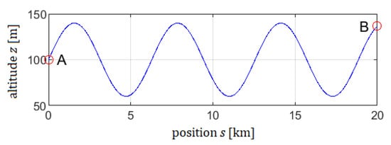
A train is driven from Station A at to Station B at . The altitude is given by ; see Figure 2. Parameters are set according to Table 2, no speed limit is assumed, and we set .
Figure 2.
Track altitude in Example 1.
Table 2.
Parameters of Example 1.
Remark 8.
The sine-shaped altitude is only assumed here as an academic example. In fact, railway lines are typically built with a rather piecewise-linear altitude profile, since this minimises the slope. Two examples based on an existing railway line will be shown later in Section 3.2 (Example 5) and Section 3.3 (Example 6).
Remark 9.
As mentioned above, is only required to be negative, and any negative value of would result in an energy minimisation problem. is only set to as an example; this choice is not mandatory here.
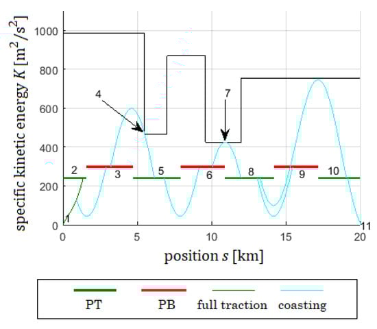
Equations (54) and (56) lead to and . Figure 3 shows the pcs-intervals calculated with Equations (58) to (61), together with the kinetic energy of the fastest motion. In our example, this leads to the exclusion of the first PT-interval since it cannot be reached.
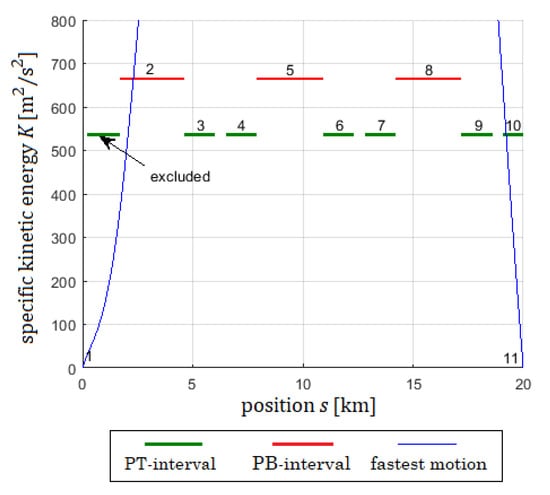
Figure 3.
Example 1: pcs-intervals PT and PB, fastest motion, and numbering.
The first step in connecting ports would be the take off from the start point at . This is the take-off case (T1). The trajectories of K and are calculated according to Equations (62) and (63). Different values of at lead to different trajectories that are shown in Figure 4 and Figure 5. When the -trajectory crosses the value 1, full traction changes to coasting, and the corresponding K-trajectory has a kink point. When the -trajectory crosses the value , coasting changes to full regenerative brake, and the corresponding K-trajectory has a kink point again. The blue line marks the only trajectory that would land on the PB-interval with number 2 (landing case (L2)). It is found by an iterative bisection of the -values at .
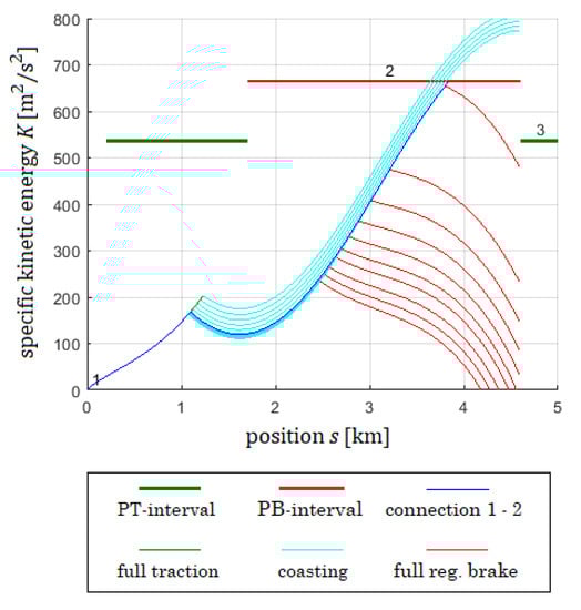
Figure 4.
Example 1: K-trajectories starting from (port 1) for various values of at . Trajectories change from full traction to coasting and then to full regenerative braking. The blue trajectory connects port 1 with port 2.
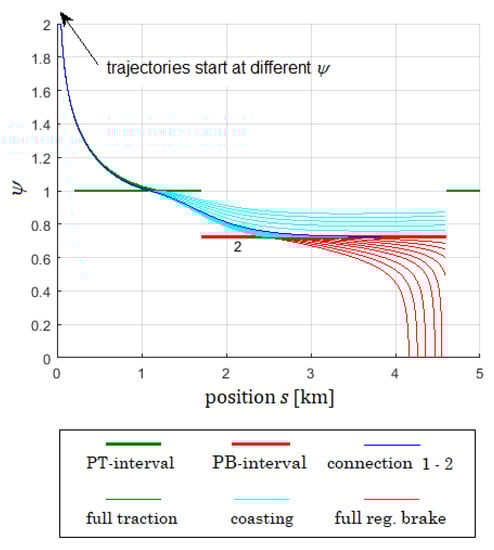
Figure 5.
Example 1: -trajectories starting from (port 1) for various values of at . Trajectories change from full traction to coasting and then to full regenerative braking. The blue trajectory connects port 1 with port 2.
Figure 6 and Figure 7 show the take off from the PT-interval number 3. This is the take-off case (T2). On the interval, the trajectories show an unstable behaviour with respect to . If is slightly above the value of 1, both K and will move upwards. If is slightly below the value of 1, both K and will move downwards. Note that takes off tangentially on the entire interval while K does so only from the ends of the interval. Close to the right end of the interval, the upwards moving K- and -trajectories will soon turn downwards, and by that change the driving modus from full traction to coasting. This is a typical picture for the take off from PT- to PB-intervals.

Figure 6.
Example 1: K-trajectories starting from PT-interval with number 3.
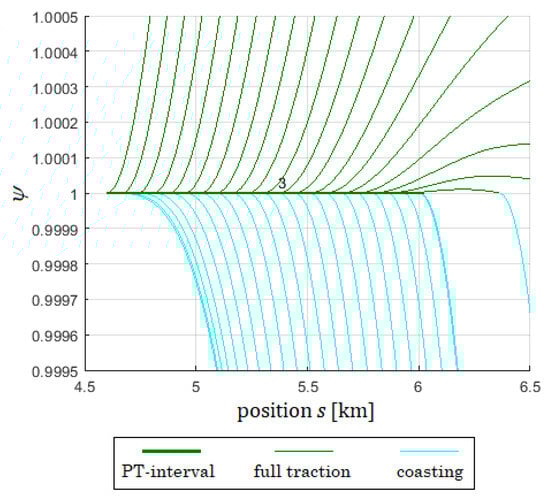
Figure 7.
Example 1: -trajectories starting from PT-interval with number 3.
Figure 8 and Figure 9 show the K- and -trajectories when trying to connect intervals 4 and 8. The K-trajectories have a kink point when the driving modus changes from coasting to full traction or full regenerative brake, corresponding to crossing the values 1 or . Both the K- and -trajectories are able to cross pcs-intervals, but the trajectory field often splits at pcs-intervals, as here at interval 7, where a shadowed region lies behind that cannot be reached by the trajectories.
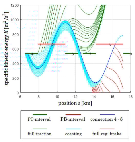
Figure 8.
Example 1: K-trajectories starting from interval 4, heading for interval 8.
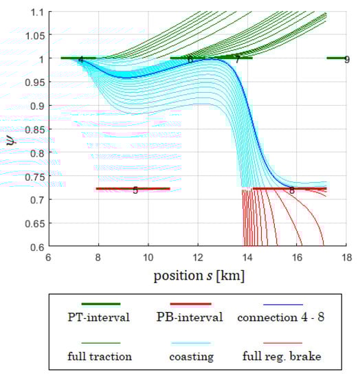
Figure 9.
Example 1: -trajectories starting from interval 4, heading for interval 8.
Remark 10.
There is great potential for speeding up the algorithm by the detection of those shadowed regions. For example, one can conclude immediately from Figure 4 that interval 3 cannot be reached from starting point 1, and from Figure 8 that interval 9 cannot be reached from interval 4. When solving the optimisation problem, it will always pay off to invest in good statistics, showing which connections should be checked and which ones can safely be excluded.
Example 2.
We consider Example 1, but now with a speed limit according to Table 3.
Table 3.
Speed limit in Example 2.
The multiplier is again set to . Figure 10, Figure 11 and Figure 12 show that all types of pcs-intervals occur. The speed limit touchpoints 4, 10, and 14 have been inserted during the run of the algorithm.
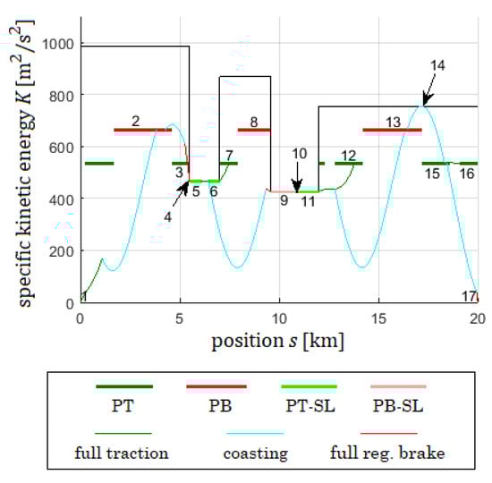
Figure 10.
Example 2: K-trajectories.
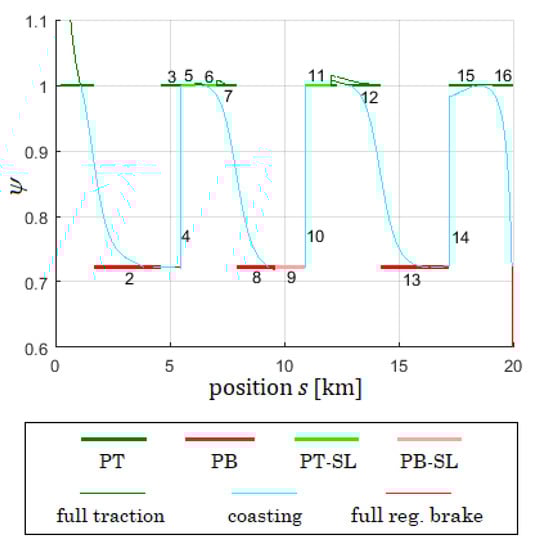
Figure 11.
Example 2: -trajectories.
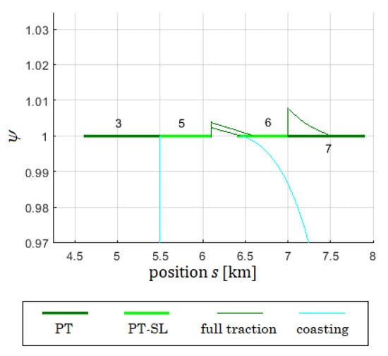
Figure 12.
Example 2: Zoom into -trajectories.
Table 4 shows the possible port connections in Example 2.
Table 4.
Port connections in Example 2.
It was shown by Khmelnitsky [18] that there always exists a unique connection from the start point (1) to the stop point (here, 17). In Example 2, this is the connection . The total time required on this connection is not known a priori, but can be calculated from the K-curve. Since is the specific kinetic energy,
holds.
Remark 11.
Here, we distinguish between the scheduled time T and the time that is evaluated from the algorithm. The final goal of the algorithm is to match to the prescribed T by a variation of . This will be explained in Section 2.5.
Example 3.
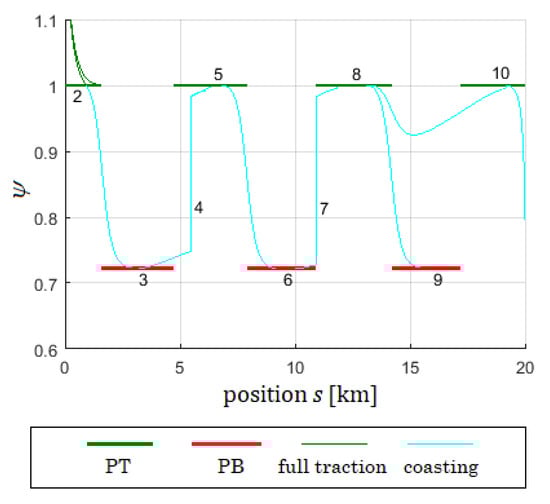
We consider Example 2, but now with . Trajectories of K and ψ are illustrated in Figure 13 and Figure 14, respectively.
Figure 13.
Example 3: K-trajectories.
Figure 14.
Example 3: -trajectories.
Table 5.
Port connections in Example 3.
2.5. The Algorithm of Khmelnitsky: Variation of the Multiplier
Khmelnitsky [18] has shown that the time between two stops of the train is a strictly monotonously increasing function of the Lagrange multiplier . Moreover, and
hold. Therefore, whenever the scheduled time T is possible to be driven on a track section by a particular train, it can be approached by the optimisation algorithm by adjusting with iterative bisection. The complete algorithm for the minimum energy operation would read as follows:
Consider a track section with stops at and to be driven in a scheduled duration T.
- Step 1: Calculate the fastest possible motion on the track section with purely regenerative braking. If the time needed for that is larger than the scheduled time T, add mechanical braking and leave the algorithm. If , choose an arbitrary negative value for and proceed with Step 2 in the algorithm.
- Step 3: Try to connect ports by regular motion with Equations (62) and (63). Use one of the take-off cases (T1)–(T8) and one of the landing cases (L1)–(L10). Add speed limit touchpoints if necessary, according to the instructions given above. Step 3 is complete when a connection from the start point at to the stop point has been found.
- Step 4: Calculate according to (66). If is sufficiently close to T, the algorithm is successfully completed. If not, adjust and proceed with Step 2.
If n is the number of ports then a maximum of possible connections has to be checked, unless the start–stop connection is found earlier. This means that the number of possible connections grows quadratically with n. The algorithm can be considered as a search tree, with port connections being the branches of the tree that need to be checked. Therefore, it is crucial to follow a clever search strategy to keep computing time at an acceptable level. We mention four important measures that dramatically shortened computing time when the code was developed:
Parallel path exclusion. Khmelnitsky [18] has proven that any two ports can only be connected by at most one path. Therefore, it is wise to exclude all parallel paths in the search tree. For example, if a connection is established, the parallel direct link is not possible and need not be checked.
Start from the treetop. When choosing the next connection to check for in Step 3, start at the highest port number that is connected to port 1 and not a known dead end. This strategy usually leads to an early discovery of the start–stop connection.
Look out for shadowed ports. If ports lie in shadow, exclude impossible connections. See the remark in the discussion of Example 1 in Section 2.3.
Estimate by interpolation. The adjustment of in Step 4 can be sped up using interpolation techniques.
Example 4.
Example 4 is equal to Examples 2 and 3, except that is not prescribed, and T is set to 16 min.
Applying the algorithm, converges to . The final K- and -trajectories are shown in Figure 15 and Figure 16.
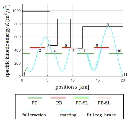
Figure 15.
Example 4: K-trajectories.
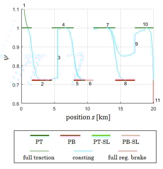
Figure 16.
Example 4: -trajectories.
Connections and types of take off and landing are given for the final value in Table 6.
Table 6.
Port connections in Example 4 at final value .
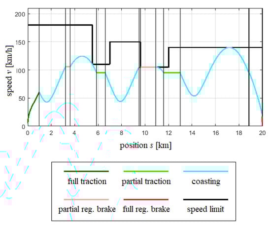
Figure 17.
Example 4: train speed.
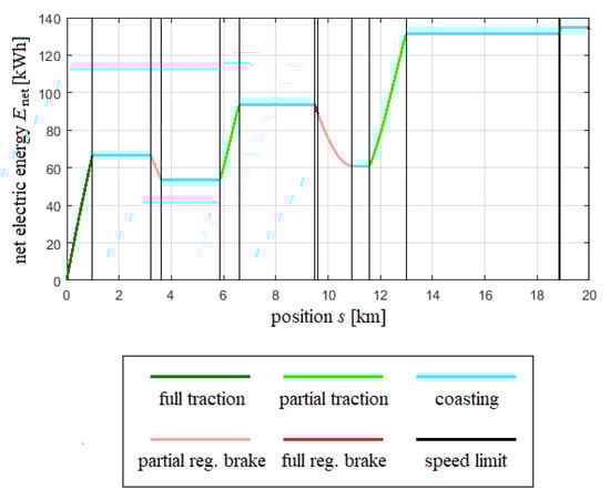
Figure 18.
Example 4: net electric energy.
3. Results and Discussion
3.1. Estimating the Potential of Efficient Train Driving
In order to compare the optimal driving performance to the energy demand of trains in a real-life operation, a study was carried out covering a total of 100 regional train runs on four track sections in Germany. The trains were drawn by electric locomotives equipped with regenerative braking. Time, velocity, energy supply from the catenary, and energy return by regenerative braking have been recorded. Trains with five, six, or seven coaches were included in the study. Train runs affected by speed restriction due to signalling in the interior of the track section have been excluded.
The total energy demand is defined by , where is the electric energy used for traction, is the electric energy returned by regenerative braking, and is an additional energy demand that is used, e.g., for air-conditioning, pressurised air, ventilation, etc. Recorded data are the energy supply and the energy return . Both traction energy and brake energy can also be computed from the measured velocity using the model given in Section 2.1, and it is interesting to compare the measured energy quantities with the ones calculated from the model. However, a direct comparison of energy return with the regenerative brake energy was difficult since the energy return turned out to be generally far less than the potential of the brake energy calculated from the model. This indicates that in many cases the regenerative brake was little used by the train drivers. A comparison of energy supply, on the other hand, had to deal with the problem that the additional energy was not recorded separately from traction energy . Therefore, we have fitted the unknown additional energy such that the measured energy supply comes close to the energy supply derived from the model. This leads to the estimate of . The comparison of energy supply is shown in Figure 19.
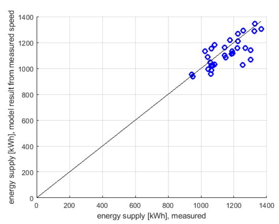
Figure 19.
Comparison of energy supply ; measurement vs. model.
Result. The energy supply was fitted to lie close to the equality line. The graph still shows that the model and measurement do not perfectly agree. This could be due to the following reasons:
- The additional energy demand might differ from one train to another.
- Wind conditions are not accounted for.
- The engine efficiency is simplified in the model to be a constant; speed and force dependent efficiency is not considered.
In the following study, we will compare the measured energy demand to the energy optimum derived by the algorithm. In this study, it would not be appropriate to compare the energy demand of a particular train run to the energy optimum based on the duration given by the timetable. Trains that are delayed need to drive faster; thus, the shorter time they have available needs to be considered in the optimum calculation. On the other hand, trains that arrive early are judged to unnecessarily waste energy by driving too fast. Therefore, for each train run, a reference time is considered that allows a fair comparison to the optimum. Let
- be the departure time according to the timetable;
- be the arrival time according to the timetable;
- be the recorded departure time, and
- be the recorded arrival time of the train run.
Then, the reference time duration is defined by , and the energy optimum is calculated with respect to this reference time. Figure 20, Figure 21, Figure 22 and Figure 23 display the total energy over the reference time T. The stars in the figures are recorded measurements, while the lines indicate the calculated energy optimum.
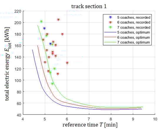
Figure 20.
Total energy demand over reference time T for track in Section 1.
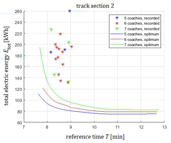
Figure 21.
Total energy demand over reference time T for track Section 2.
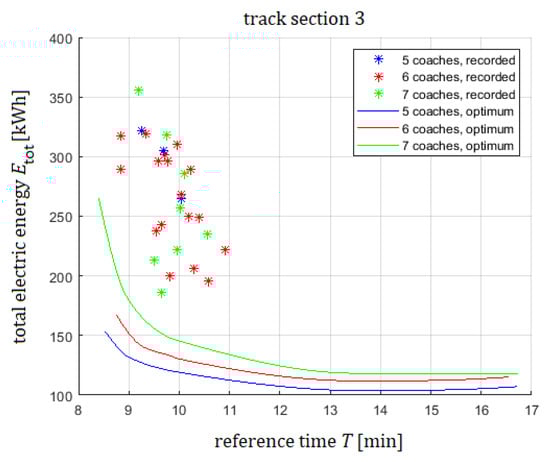
Figure 22.
Total energy demand over reference time T for track in Section 3.
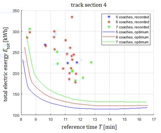
Figure 23.
Total energy demand over reference time T for track in Section 4.
Result. Figure 20, Figure 21, Figure 22 and Figure 23 show that the recorded total energy spreads over a rather wide range. A factor of approximately two lies between the minimum and maximum energy consumption on each track section, even for cases with a quite similar reference time. Contrary to the expectation, the recorded values do not show an increase in energy demand with train length, but this might be due to the small size of the sample and the wide spread of values. For many train runs, the measured energy is far above the corresponding optimum line, in some extremal cases by a factor of three.
Remark 12.
In one case shown in Figure 20, a seven-coach train was in fact better than the optimum. This is not a contradiction to the optimality property. As was pointed out, the optimal control theory ensures that the algorithm returns the energy minimum, but this only holds for the given train motion model. This model is only a simplification, and some assumptions might not have been met during the train drive experiment. For example, wind speed is neither measured nor considered in the model, and the additional energy requirement is only averaged for a lack of individual measurements.
If, for the i-th train run, the recorded total energy is denoted by , and the corresponding optimum energy is , then the energy ratio can be evaluated. Within the concept of the Physical Optimum (PhO) [55,56], is called a PhO factor that quantitatively evaluates the efficiency with respect to a feasible and most efficient reference process. This energy ratio is shown in Figure 24 for each of the 100 train runs of the study. A total energy ratio is obtained by summing over all train runs studied. This can be seen as an estimate of the potential that energy optimised driving would have. Based on the results of the present study, an amount of 37.3 percent of energy could be saved by following an energy minimising driving strategy. One should, however, bear in mind two limitations: First, due to model simplifications, the computed driving strategy might differ from the real optimum under the current conditions. Secondly, even if an optimum strategy is displayed to the driver by an assistance system, it can only be approached, and interactions with other traffic will sometimes not allow one to exactly follow the suggestions. However, since the theoretical optimum turned out to be substantially lower than the measured energy demand in operation, we think that there is still a large potential for energy saving by the optimal control-based assistance for train drivers.
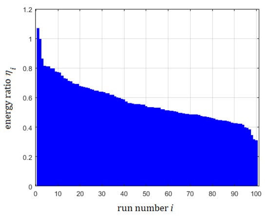
Figure 24.
Energy ratio for each run, shown in descending order.
3.2. Sensitivity to Deviations from the Optimum Driving Profile
In this section, it is studied how deviations from the optimum driving profile will increase the energy requirement. The effect is shown using the following example.
Example 5.
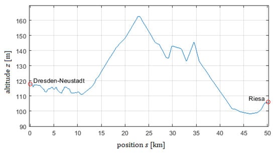
We consider the railway section between Dresden-Neustadt and Riesa. Both stations are located on the Dresden–Leipzig line in Germany. The altitude of the section is shown in Figure 25. Train parameters are the same as in Examples 1–4, see Table 2. The only difference to Examples 1–4 is that now an additional energy requirement is assumed. The total time T is set to 22 min. Speed limits are not assumed in this example.
Figure 25.
Example 5: track altitude z.
After calculation of the optimum driving profile, seven neighbouring trajectories are constructed, called variant 1 to variant 7. Every variant is driven with the same train parameters on the same track, and the total time needed is equal for every variant. Variants 1–3 are too fast at the beginning. Then, at a certain position, the speed of each variant is corrected such that it will still arrive at the scheduled total time of 22 min. On the other hand, variants 4–7 are too slow at the beginning. Variant 4 manages to arrive at the prescribed time by completely avoiding the coasting regime. Variants 5–7 accelerate at certain positions and then switch to coasting. In order not to overload the figures, we first show the comparison of variant 1–3 to the optimum in Figure 26, Figure 27 and Figure 28 and proceed then with variant 4–7 versus the optimum in Figure 29, Figure 30 and Figure 31.
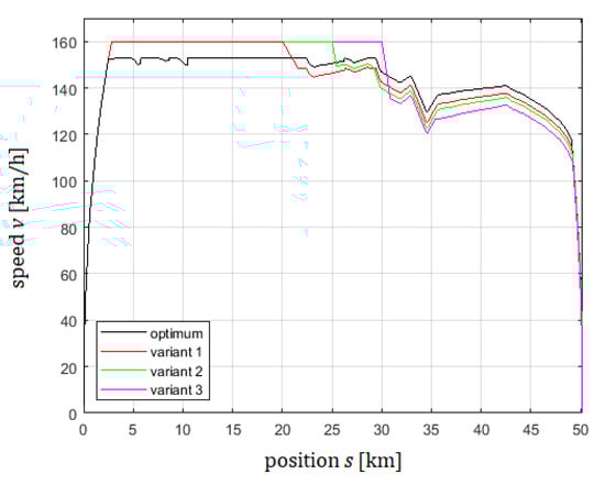
Figure 26.
Example 5: train speed v (optimum and variants 1–3).
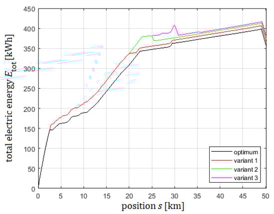
Figure 27.
Example 5: total electric energy (optimum and variants 1–3).

Figure 28.
Example 5: total electric energy (optimum and variants 1–3). Zoom into Figure 27.
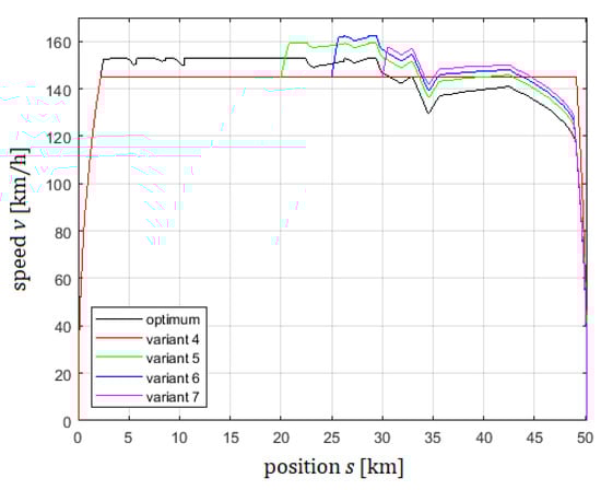
Figure 29.
Example 5: train speed v (optimum and variants 4–7).
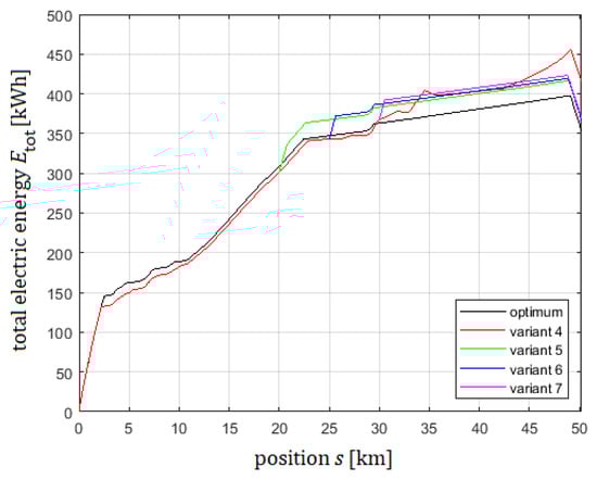
Figure 30.
Example 5: total electric energy (optimum and variants 4–7).

Figure 31.
Example 5: total electric energy (optimum and variants 4–7). Zoom into Figure 30.
Result. The total electric energy demand is compared
As could be expected, the optimum driving strategy indeed leads to a minimum value of at arrival. However, most variants studied here require only slightly more total electric energy. An exception is variant 4 that has no coasting section included and needs substantially more energy. The values of and percentages are given in Table 7.
Table 7.
Electric energy demand at arrival for optimum strategy and variants 1–7.
Remark 13.
In fact it would be easy to construct driving strategies that are far worse than the ones considered here, for example driving with frequent switching between acceleration and braking, but this was not the focus of our study. It was our intention to compare the optimum to some variants that are still quite reasonable. Most of the variants perform quite well, since from the end point of their cruising period on, they are constructed such that they actually continue in an optimum way. The ‘good news’ from this study is that, whenever a deviation from optimum is noticed early enough, counteraction by following a recalculated optimum profile will keep the error small.
3.3. Influence of the Total Recuperation Efficiency on the Optimum Driving Profile
As the total recuperation efficiency is directly included in the maximisation problem, Equation (19), it can be expected that a variation of leads to a certain change in the optimum driving strategy. In this section, the effect of on the optimum speed profile is briefly illustrated in a numerical example.
Example 6.
Example 6 is equal to Example 5 (Dresden-Neustadt—Riesa) except for the following changes: (1) The total time T is set to 23 min. (2) A speed limit is considered according to Table 8. (3) The efficiency of the regenerative brake will be varied.
Table 8.
Speed limit in Example 6.
The optimum train driving profiles are calculated for three values of . The resulting curves for speed v and total electric energy are shown in Figure 32 and Figure 33, respectively.
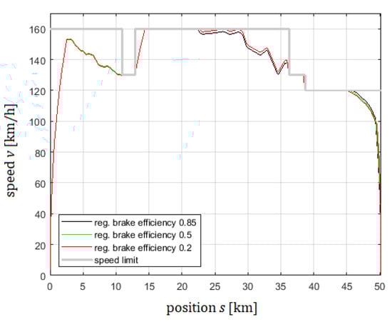
Figure 32.
Example 6: train speed v for different regenerative brake efficiency .
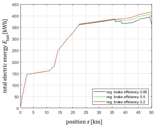
Figure 33.
Example 6: total electric energy for different regenerative brake efficiency .
Result. A small effect of different recuperation efficiency on speed is visible during the coasting periods. The position where coasting starts is slightly different. The effect on total energy is much more pronounced due to the different amount of recuperation energy.
Example 6 is only meant to show that a certain (but small) effect on speed could be observed. Braking regimes lead to different energy losses when the recuperation efficiency changes. This can result in different optimum speed profiles. A deeper analysis of this subject is beyond the focus of this study.
4. Conclusions
Within this paper, energy-efficient train driving has been studied for the case of an exclusive usage of the regenerative brake in electric trains. The code Leda written at Fraunhofer Institute Magdeburg is based on the algorithm of Khmelnitsky that constructs the unique minimum energy solution. A derivation of the statements given by Khmelnitsky from a more general formulation of Pontryagin’s maximum principle is presented. In addition to the theory in Khmelnitsky’s article, a complete list of switching cases was provided and illustrated by a number of numerical examples. A comparison to energy consumption data in a real operation showed that the energy minimising strategy was able to save, on average, about 37% of energy. A study of some sub-optimum driving profiles showed, in most cases, only moderate energy loss when deviations are corrected using a recalculated optimum. A slight influence of regenerative brake efficiency on the optimum speed profile was detected in a numerical example.
Extensions of the code to include mechanical braking, non-zero speed boundary conditions, and dynamic response to train delays are subject to further research.
Author Contributions
Writing—original draft preparation, W.H.; software, W.H.; project administration, M.R. and T.B.-R.; funding acquisition, M.R. and T.B.-R. All authors have read and agreed to the published version of the manuscript.
Funding
The authors gratefully acknowledge external funding by the Federal Office for Economic Affairs and Export Control (Bundesamt für Wirtschaft und Ausfuhrkontrolle) of Germany within the pilot programme ‘Einsparzähler’.
Data Availability Statement
External data that have been processed cannot be provided nor referenced for confidentiality reasons.
Acknowledgments
The authors would like to thank the team of traveltainer GmbH & Co. KG, Altenbeken, Germany for their valuable collaboration and support during this research project.
Conflicts of Interest
The authors declare no conflict of interest.
Abbreviations
The following abbreviations are used in this manuscript:
| DDP | Discrete dynamic programming |
| EETC | Energy-efficient train control |
| KKT | Karush–Kuhn–Tucker (conditions) |
| NLP | Nonlinear programming |
| PB | Partial regenerative braking |
| PB-SL | Partial regenerative braking at speed limit |
| pcs-interval | Possible constant speed interval |
| PMP | Pontryagin maximum principle |
| PT | Partial traction |
| PT-SL | Partial traction at speed limit |
| SL-TP | Speed limit touchpoint |
| SNCF | Société nationale des chemins de fer français (French national railways) |
| TGV | Train à grande vitesse (French high-speed train) |
References
- Strobel, H.; Horn, P.; Kosemund, M. Contribution to optimum computer-aided control of train operation. In Proceedings of the 2nd IFAC/IFIP/IFORS Symposium on Traffic Control and Transportation Systems, Monte Carlo, Monaco, 16–21 September 1974; pp. 377–387. [Google Scholar]
- Howlett, P.G.; Pudney, P.J. Energy-Efficient Train Control; Springer: London, UK, 1995. [Google Scholar]
- Franke, R.; Terwiesch, P.; Meyer, M. An algorithm for the optimal control of the driving of trains. In Proceedings of the 39th IEEE Conference on Decision and Control, Sydney, Australia, 12–15 December 2000; Volume 3. [Google Scholar]
- Albrecht, T. Ein Beitrag zur Nutzbarmachung Genetischer Algorithmen für die Optimale Steuerung und Planung eines Flexiblen Stadtschnellbahnbetriebes (A Contribution to the Utilization of Genetic Algorithms for Optimal Control and Planning of a Flexible Urban Rail Transport). Ph.D. Thesis, Dresden University of Technology, Dresden, Germany, 2005. [Google Scholar]
- Howlett, P.G.; Pudney, P.J.; Vu, X. Freightmiser: An energy-efficient application of the train control problem. In Proceedings of the 30th Conference of Australian Institutes of Transport Research (CAITR), Perth, Australia, 10–12 December 2008. [Google Scholar]
- Aradi, S.; Becsi, T.; Gaspar, P. A predictive optimization method for energy-optimal speed profile generation for trains. In Proceedings of the 2013 IEEE 14th International Symposium on Computational Intelligence and Informatics (CINTI), Budapest, Hungary, 19–21 November 2013. [Google Scholar]
- DAS on-Board Algorithms. Technical Report D6.3, ON-TIME: Optimal Networks for Train Integration Management across Europe. 2014. Available online: https://cordis.europa.eu/project/id/285243 (accessed on 9 September 2023).
- Albrecht, A.R.; Howlett, P.G.; Pudney, P.J.; Vu, X.; Zhou, P. Energy-efficient train control: The two-train separation problem on level track. J. Rail Transp. Plan. Manag. 2015, 5, 163–182. [Google Scholar] [CrossRef]
- Scheepmaker, G.; Goverde, R.; Kroon, L. Review of energy-efficient train control and timetabling. Eur. J. Oper. Res. 2017, 257, 355–376. [Google Scholar] [CrossRef]
- Pontryagin, L.; Boltyanskii, V.; Gamkrelidze, R.; Mishchenko, E. Matematicheskaya Teoriya Optimal’nykh Prozessov; Fizmatgiz: Moscow, Russia, 1961. [Google Scholar]
- Pontryagin, L.; Boltyanskii, V.; Gamkrelidze, R.; Mishchenko, E. The Mathematical Theory of Optimal Processes; John Wiley and Sons (Interscience Publishers): New York, NY, USA, 1962. [Google Scholar]
- Ichikawa, K. Application of optimization theory for bounded state variable problems to the operation of train. Bull. Jpn. Soc. Mech. Eng. 1968, 11, 857–865. [Google Scholar] [CrossRef]
- Milroy, I.P. Aspects of Automatic Train Control. Ph.D. Thesis, Loughborough University, Loughborough, UK, 1980. [Google Scholar]
- Howlett, P.G.; Milroy, I.P.; Pudney, P.J. Energy-efficient train control. Control Eng. Pract. 1994, 2, 193–200. [Google Scholar] [CrossRef]
- Liu, R.R.; Golovitcher, I.M. Energy-efficient operation of rail vehicles. Transp. Res. Part A Policy Pract. 2003, 37, 917–932. [Google Scholar] [CrossRef]
- Albrecht, A.R.; Howlett, P.G.; Pudney, P.J.; Vu, X. Energy-efficient train control: From local convexity to global optimization and uniqueness. Automatica 2003, 49, 3072–3078. [Google Scholar] [CrossRef]
- Asnis, I.A.; Dmitruk, A.V.; Osmolovskii, N.P. Solution of the problem of the energetically optimal control of the motion of a train by the maximum principle. USSR Comput. Math. Math. Phys. 1985, 25, 37–44. [Google Scholar] [CrossRef]
- Khmelnitsky, E. On an Optimal Control Problem of Train Operation. IEEE Trans. Autom. Control 2000, 45, 1257–1266. [Google Scholar] [CrossRef]
- Ying, P.; Zeng, X.; Song, H.; Shen, T.; Yuan, T. Energy-efficient train operation with steep track and speed limits: A novel Pontryagin’s maximum principle-based approach for adjoint variable discontinuity cases. IET Intell. Transp. Syst. 2021, 15, 1183–1202. [Google Scholar] [CrossRef]
- Ying, P.; Zeng, X.; Shen, T.; Wang, Y.; Ma, Z.; Wu, Y. Partial Train Speed Trajectory Optimization. In Proceedings of the 2022 IEEE 25th International Conference on Intelligent Transportation Systems (ITSC), Macau, China, 8–12 October 2022. [Google Scholar]
- Baranov, L.A.; Meleshin, I.S.; Chin’, L.M. Optimal control of a subway train with regard to the criteria of minimum energy consumption. Russ. Electr. Eng. 2011, 82, 405–410. [Google Scholar] [CrossRef]
- Lu, S.; Weston, P.; Hillmansen, S.; Gooi, H.; Roberts, C. Increasing the regenerative braking energy for railway vehicles. IEEE Trans. Intell. Transp. Syst. 2014, 15, 2506–2515. [Google Scholar] [CrossRef]
- Zhou, Y.; Bai, Y.; Li, J.; Mao, B.; Li, T. Integrated optimization on train control and timetable to minimize net energy consumption of metro lines. J. Adv. Transp. 2018, 2018, 7905820. [Google Scholar] [CrossRef]
- Fernández-Rodríguez, A.; Fernández-Cardador, A.; Cucala, A. Real time eco-driving of high speed trains by simulation-based dynamic multi-objective optimization. Simul. Model. Pract. Theory 2018, 84, 50–68. [Google Scholar] [CrossRef]
- Scheepmaker, G.; Goverde, R. Energy-efficient train control using nonlinear bounded regenerative braking. Transp. Res. Part C Emerg. Technol. 2020, 121, 102852. [Google Scholar] [CrossRef]
- Rao, A.; Benson, D.; Darby, C.; Patterson, M.; Francolin, C.; Sanders, I.; Huntington, G. Algorithm 902: GPOPS, a MATLAB software for solving multiple-phase optimal control problems using the Gauss pseudospectral method. ACM Trans. Math. Softw. 2010, 37, 22:1–22:39. [Google Scholar] [CrossRef]
- Su, S.; Tang, T.; Li, X. Driving strategy optimization for trains in subway systems. Proc. Inst. Mech. Eng. Part F J. Rail Rapid Transit 2018, 232, 369–383. [Google Scholar] [CrossRef]
- Zhu, Q.; Su, S.; Tang, T.; Liu, W.; Zhang, Z.; Tian, Q. An eco-driving algorithm for trains through distributing energy: A Q-Learning approach. ISA Trans. 2022, 122, 24–37. [Google Scholar] [CrossRef]
- Su, S.; Zhu, Q.; Liu, J.; Tang, T.; Wei, Q.; Cao, Y. A Data-Driven Iterative Learning Approach for Optimizing the Train Control Strategy. IEEE Trans. Ind. Inform. 2023, 19, 7885–7893. [Google Scholar] [CrossRef]
- Ghaviha, N.; Bohlin, M.; Holmberg, C.; Dahlquist, E.; Skoglund, R.; Jonasson, D. A driver advisory system with dynamic losses for passenger electric multiple units. Transp. Res. Part C Emerg. Technol. 2017, 85, 111–130. [Google Scholar] [CrossRef]
- Kouzoupis, D.; Pendharkar, I.; Frey, J.; Diehl, M.; Corman, F. Direct multiple shooting for computationally efficient train trajectory optimization. Transp. Res. Part C Emerg. Technol. 2023, 152, 104170. [Google Scholar] [CrossRef]
- Feng, M.; Huang, Y.; Lu, S. Eco-driving Strategy Optimization for High-speed Railways Considering Dynamic Traction System Efficiency. IEEE Trans. Transp. Electrif. 2023. early access. [Google Scholar] [CrossRef]
- Cao, Y.; Zhang, Z.; Cheng, F.; Su, S. Trajectory Optimization for High-Speed Trains via a Mixed Integer Linear Programming Approach. IEEE Trans. Intell. Transp. Syst. 2022, 23, 17666–17676. [Google Scholar] [CrossRef]
- Zhang, Z.; Cao, Y.; Su, S. Energy-Efficient Driving Strategy for High-Speed Trains with Considering the Checkpoints. Chin. J. Electron. 2023, in press. [Google Scholar]
- Szkopiński, J.; Kochan, A. Energy Efficiency and Smooth Running of a Train on the Route While Approaching Another Train. Energies 2021, 14, 7593. [Google Scholar] [CrossRef]
- Su, S.; Tang, T.; Chen, L.; Liu, B. Energy-efficient train control in urban rail transit systems. Proc. Inst. Mech. Eng. Part F J. Rail Rapid Transit 2015, 229, 446–454. [Google Scholar] [CrossRef]
- Fernández-Rodríguez, A.; Su, S.; Fernández-Cardador, A.; Cucala, A.P.; Cao, Y. A multi-objective algorithm for train driving energy reduction with multiple time targets. Eng. Optim. 2021, 53, 719–734. [Google Scholar] [CrossRef]
- Wang, Y.; Schutter, B.; van den Boom, T.; Ning, B. Optimal trajectory planning for trains—A pseudospectral method and a mixed integer linear programming approach. Transp. Res. Part C Emerg. Technol. 2013, 29, 97–114. [Google Scholar] [CrossRef]
- DIDO Optimal Control Software. Elissar Global. Available online: https://www.mathworks.com/products/connections/product_detail/dido.html (accessed on 9 September 2023).
- Ross, I.; Karpenko, M. A review of pseudospectral optimal control: From theory to flight. Annu. Rev. Control 2012, 36, 182–197. [Google Scholar] [CrossRef]
- Ross, I. A Primer on Pontryagin’s Principle in Optimal Control; Collegiate Publishers: San Francisco, CA, USA, 2015. [Google Scholar]
- PSOPT Optimal Control Software. Available online: https://www.psopt.net/ (accessed on 9 September 2023).
- Becerra, V. Solving complex optimal control problems at no cost with psopt. In Proceedings of the 2010 IEEE International Symposium on Computer-Aided Control System Design, Yokohama, Japan, 8–10 September 2010; pp. 1391–1396. [Google Scholar]
- GPOPS-II: Next-Generation Optimal Control Software. Available online: http://gpops2.com/ (accessed on 9 September 2023).
- Hartl, R.; Sethi, S.; Vickson, R. A survey of the maximum principles for optimal control problems with state constraints. SIAM Rev. 1995, 37, 181–218. [Google Scholar] [CrossRef]
- Ihme, J. Schienenfahrzeugtechnik; Springer Fachmedien: Wiesbaden, Germany, 2016. [Google Scholar]
- Fassbinder, S. Wie Energie-Effizient ist der Bahnverkehr Wirklich? Technical Report, Deutsches Kupferinstitut, Düsseldorf. 2010. Available online: https://de.slideshare.net/LeonardoENERGYDeutschland/wie-energieeffizient-ist-der-bahnverkehr-wirklich (accessed on 9 September 2023).
- Curtius, E.; Kniffler, A. Neue Erkenntnisse über Haftung zwischen Treibrad und Schiene. Elektrische Bahnen 1944, 20, 25–30. [Google Scholar]
- Schlecht, B. Maschinenelemente 2; Pearson Studium: Munich, Germany, 2010. [Google Scholar]
- Wie “grün” ist der Schienenverkehr? Technical Report, Deutsches Kupferinstitut, Düsseldorf. 2020. Available online: https://www.kupferinstitut.de/wp-content/uploads/2020/02/BahnEffizienz.pdf (accessed on 9 September 2023).
- Frilli, A.; Meli, E.; Nocciolini, D.; Pugi, L.; Rindi, A. Energetic optimization of regenerative braking for high speed railway systems. Energy Convers. Manag. 2016, 129, 200–215. [Google Scholar] [CrossRef]
- Voß, G.; Gackenholz, L.; Wiebels, R. Eine neue Formel (Hannoversche Formel) zur Bestimmung des Luftwiderstandes spurgebundener Fahrzeuge. Glas. Annalen–Zeitschrift Für Eisenbahnwesen Und Verkehrstechnik 1972, 96, 166–171. [Google Scholar]
- Karush, W. Minima of Functions of Several Variables with Inequalities as Side Constraints. Master’s Thesis, University of Chicago, Chicago, IL, USA, 1939. [Google Scholar]
- Kuhn, H.; Tucker, A. Nonlinear Programming. In Proceedings of the 2nd Berkeley Symposium on Mathematical Statististics and Probability, Berkeley, CA, USA, 31 July–12 August 1950; pp. 481–492. [Google Scholar]
- Volta, D. Das Physikalische Optimum als Basis von Systematiken zur Steigerung der Energie-und Stoffeffizienz von Produktionsprozessen. Ph.D. Thesis, Clausthal University of Technology, Clausthal-Zellerfeld, Germany, 2014. [Google Scholar]
- Eggers, N.; Böttger, J.; Kerpen, L.; Sankol, B.; Birth, T. Refining VDI guideline 4663 to evaluate the efficiency of a power-to-gas process by employing limit-oriented indicators. Energy Effic. 2021, 14, 73. [Google Scholar] [CrossRef]
Disclaimer/Publisher’s Note: The statements, opinions and data contained in all publications are solely those of the individual author(s) and contributor(s) and not of MDPI and/or the editor(s). MDPI and/or the editor(s) disclaim responsibility for any injury to people or property resulting from any ideas, methods, instructions or products referred to in the content. |
© 2023 by the authors. Licensee MDPI, Basel, Switzerland. This article is an open access article distributed under the terms and conditions of the Creative Commons Attribution (CC BY) license (https://creativecommons.org/licenses/by/4.0/).