Abstract
In light of the nonlinearity, high dimensionality, and time-varying nature of the operational conditions of the pulverizer in power plants, as well as the challenge of the real-time monitoring of quality variables in the process, a data-driven KPCA–Bagging–GMR framework for soft sensors using reduced dimensions and ensemble learning is proposed. Firstly, the methodology employs a Kernel Principal Component Analysis to effectively reduce the dimensionality of the collected process data in a nonlinear manner. Secondly, the reduced principal components are then utilized to reconstruct a refined set of input samples, followed by the application of the Bagging algorithm to obtain multiple subsets of the samples and develop corresponding Gaussian Mixture Regression models. Ultimately, the fusion output is achieved by calculating the weights of each local model based on Bayesian posterior probabilities. By conducting simulation experiments on the coal mill, the proposed approach has been validated as demonstrating superior predictive accuracy and excellent generalization capabilities.
1. Introduction
With the rapid development of the power industry, the pulverizers in power plants play a crucial role in ensuring stable power supply and efficient operation [1,2]. To guarantee the high performance and safe operation of pulverizers, researchers have begun to explore accurate predictions of their performance and fault conditions [3,4,5]. However, due to the complexity and nonlinearity of the pulverizer, traditional modeling methods often struggle to capture their underlying patterns and characteristics, resulting in a low prediction accuracy. The introduction of ensemble learning methods [6,7,8] provides an effective solution for modeling pulverizers in power plants. By integrating the predictions of multiple individual models, ensemble learning can enhance the prediction capability of running conditions and fault situations of pulverizers. As a result, ensemble learning methods gradually became a research hot spot for modeling pulverizers in the power industry.
The basic idea behind ensemble learning is to combine the predictions of multiple individual models to improve overall prediction performance. In the modeling of pulverizers, various modeling methods can be employed to construct individual models, such as Support Vector Machines (SVM) [9,10], Artificial Neural Networks (ANN) [11,12], Decision Trees (DT) [13], and others [14,15,16]. Each individual model can capture different features and patterns of pulverizers, thereby providing more comprehensive and accurate predictions. The key to ensemble learning lies not only in appropriate combination methods but also in considering the diversity and accuracy among individual models [17,18]. Diversity can be achieved by applying different feature selection methods, model structures, or training data, which provides more information to address modeling problems. On the other hand, the accuracy of individual models relies on their own performance, including accuracy, generalization ability, etc. Thus, in the application of ensemble learning methods, there is a need to balance the relationship between diversity and accuracy.
To achieve diversity, several aspects can be considered. Firstly, different feature selection methods can be utilized to construct individual models, allowing each model to focus on different features and thereby enhancing the overall model diversity [19]. Secondly, various model structures, such as SVM, ANN, and DT, can be chosen to introduce differences in learning and expressive capabilities among individual models, thereby enhancing the diversity of the ensemble model [20]. Additionally, diverse information and diversity can be obtained using different training data or training algorithms. On the other hand, the accuracy of individual models is crucial for the performance of ensemble learning. During the selection of individual models, an evaluation should be conducted based on metrics such as accuracy, generalization ability, and stability. Selecting high-performance individual models contributes to enhancing the overall prediction capability of the ensemble model. When employing ensemble learning, the correlations among individual models should also be taken into account. If there is a high degree of correlation among individual models, they may provide redundant information during the ensemble process, leading to a decrease in performance. Therefore, selecting individual models with lower correlations is essential for constructing an efficient ensemble model.
In practical applications, ensemble learning methods have achieved certain success in the modeling of pulverizers in power plants. By integrating multiple different individual models, ensemble learning can improve the prediction accuracy of pulverizer performance and fault conditions. Research has shown that in real plant operations, ensemble learning methods can more accurately capture the dynamic characteristics and fault conditions of pulverizers compared to individual models [21], thus enhancing the operational stability and efficiency of power plants. However, despite the promising application results of ensemble learning methods in the modeling of pulverizers, there are still challenges and room for improvement. Firstly, the selection and design of ensemble learning methods depend on prior knowledge and experience [22,23], requiring a certain understanding of the performance and characteristics of different models. Thus, further research is needed for the introduction and application of novel models and algorithms to investigate their applicability and effectiveness. Secondly, ensemble learning methods have higher computational complexity, particularly when dealing with large-scale data and high-dimensional features [24]. Therefore, improving the computational efficiency and scalability of ensemble learning methods is also an important research direction.
However, existing individual models in ensemble learning are based on extracting the relationship between input and output data from the original data, which inherently contain strong, noisy information. Eliminating such noise will be beneficial for reducing the difficulty of model construction and improving model accuracy. Considering the large-scale and high-dimensional characteristics of the operational data from a coal mill in power plants, this study proposes a Gaussian Mixture Regression (GMR) modeling approach based on the Kernel Principal Component Analysis (KPCA) and Bagging algorithm. KPCA is utilized to map the original data to a high-dimensional space for linearization and dimensionality reduction, eliminating the inherent noise of input data. Then, a Gaussian process regression method is employed to establish a soft sensing model. Furthermore, the Bagging ensemble approach is applied to improve the predictive accuracy and robustness of the model. In Section 2, an introduction to KPCA, the Bagging algorithm, GMR, and Bayesian information fusion methods is provided. Section 3 provides a detailed description of the KPCA–Bagging–GMR algorithm and its steps in Bayesian information fusion. In Section 4, the application of the KPCA–Bagging–GMR algorithm and its Bayesian information fusion method in coal mill data modeling in power plants is presented. A comparison with similar algorithms is conducted to validate the superiority of this approach.
2. Principle and Method
2.1. KPCA Reducing Dimensions
KPCA is a non-linear dimensionality reduction technique that represents a variant of Principal Component Analysis (PCA) [25,26]. PCA is a commonly used linear dimensionality reduction method that reduces the dimensionality of data by finding projections along the directions of maximum variance, which has been widely used in other fields [27,28,29]. In contrast, KPCA employs the use of the kernel trick to map the data into a higher dimensional feature space, where PCA is performed. The underlying principle of KPCA is to capture the non-linear structure of data by conducting PCA operations in a high-dimensional feature space. Initially, KPCA calculates the similarity among samples using a kernel function, thereby mapping the original data into a higher dimensional feature space. In this feature space, PCA can be applied to compute the principal components and generate the minimum dimensional representation. Finally, by projecting the new data back to the original space, the dimensionality-reduced data are obtained. The advantages of KPCA lie in its ability to handle non-linear data and preserve the essential structure of the data. It finds applications in tasks such as data visualization, feature extraction, and pattern recognition. However, it is computationally expensive as it involves the calculation of the kernel function and the covariance matrix in the feature space.
Assuming the sample data are set as , , is the number of samples, and m is the sample dimensionality. Let be a non-linear transformation method mapping the original data to the mapping space F. When the premise condition is satisfied, the covariance matrix of the transformed data is given as follows.
The features of covariance matrix C are decomposed as follows.
where is the eigenvalue of covariance matrix and , is the corresponding eigenvector.
Equation (2) is simultaneously left multiplied by to get the following expression.
The eigenvector corresponding to the non-zero eigenvalue can be obtained through Equation (3), as follows.
The kernel function is introduced.
where is the kernel matrix generated by kernel function and is the eigenvector corresponding to .
By substituting Equations (4) and (5) into Equation (3), the expression can be obtained as follows.
At this point, the problem of finding the eigenvalues and eigenvectors of the covariance matrix C is transformed into the problem of finding the eigenvalues and eigenvectors of the kernel function matrix . The Gaussian kernel function is used as follows.
where is the kernel width parameter. The obtained eigenvalues are sorted in descending order, and the corresponding eigenvectors are processed via unit orthogonalization. The projection of kernel matrix on some eigenvectors can be obtained by extracting the first t principal elements based on the contribution rate of principal elements.
In practice, the conclusion of may not hold, so it is necessary to modify the nuclear matrix in Equation (6), as follows.
where I is a matrix with element .
2.2. Bagging Algorithm
Bagging, namely bootstrap aggregating, is a machine learning technique that combines the weak learners to reduce the prediction errors, which was first introduced by Breiman [30]. The fundamental principle behind the Bagging algorithm entails training a weak learner multiple times using a training set. Each training set is generated by performing random sampling with replacement from the original dataset, resulting in several localized outputs. Subsequently, these individual predictions are amalgamated using a prescribed rule to derive the ultimate outcome. As each training set is acquired through the process of random sampling, it is possible that certain samples from the original dataset may be selected multiple times and subsequently appear in multiple new training sets. On the contrary, there are other samples that may not be selected at all during the sampling procedure. Through the utilization of repetitive random sampling techniques, the Bagging algorithm amplifies the heterogeneity among the learning machines, thereby enhancing the model’s capacity for generalization and precision.
The Bagging algorithm leverages repeated random sampling from the original sample set, with a total of m iterations, to construct a training set denoted as . Each sampling iteration involves the selection of b samples as , . Utilizing the learning machines, the new training set is utilized for training, resulting in the creation of B distinct local models. These local models are subsequently consolidated to yield the ultimate predictive outcome.
2.3. Gaussian Mixture Regression Model
GMR is a regression analysis approach that utilizes a Gaussian mixture model (GMM) [31]. It is a model that represents a dataset by overlaying multiple Gaussian distributions. Let and , , and represent the input and output variables of the i-th sample, where M and N represent the dimensions of the input variables and the number of training samples, respectively. The input and output data can be represented in matrix form as and . Figure 1 shows the probability graph of the Gaussian Mixture Regression model, where represents the weights of different Gaussian distributions, satisfying , and K represents the number of Gaussian distributions in the dataset. and represent the mean and covariance matrices of the Gaussian distributions, respectively. and are the regression coefficient matrix and the measurement noise variance matrix, respectively. represents the latent variables of the i-th sample, where . When = 1, it indicates that the i-th sample belongs to the k-th Gaussian distribution, thus satisfying . The joint probability distribution of the data pair and the marginal distribution of the input variable xi in the k-th Gaussian distribution are given as follows.
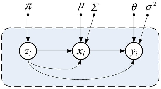
Figure 1.
Principle of GMR.
In Equations (9) and (10),
where is the functional mapping relationship between the output variable and the input variable, signifies the regression coefficients, and is Gaussian measurement noise with a mean of 0 and a variance of .
In the GMR model, the estimated model parameters to be determined consist of . Typically, the expectation–maximization algorithm (EM) based on maximizing the logarithm of the likelihood function is employed, combined with the training data, to obtain parameter estimates for the model. The EM algorithm involves two steps. In the expectation step (E-step), the posterior probability distribution p(Z|D) characterizing the latent variables representing the membership of samples to different modes is derived based on the given training sample set D. In the maximization step (M-step), the updated values for each parameter are obtained by taking the derivative of the logarithm of the likelihood function with respect to each model parameter. After iterations using the EM algorithm, parameter estimates based on the training sample D can be obtained.
For a given predictive sample, when the input variable is provided, the posterior probability distribution of the sample belonging to different modes is first computed, as follows.
By taking the expected value of the probability distribution of the output variable , the estimated result for can be obtained as follows.
As indicated by Equation (13), the GMR model no longer relies solely on the prediction output of a single global model. Instead, it assigns appropriate weights to multiple local models, considering the predictive information provided by each local model to accurately output the final result. A larger value of indicates a higher probability that the predictive sample originates from the k-th Gaussian distribution, thereby giving greater weight to the corresponding local model’s prediction result.
2.4. Bayesian Network Information Fusion
Bagging algorithm is employed to randomly select b samples from the training set, creating a sub-training set. This process is repeated B times to generate B training sets , which are then individually trained using the GMR method. By applying this process to the B sub-models, B predictions are simultaneously obtained.
In order to improve the accuracy of the Bagging Gaussian process regression modeling method, a posteriori probability-weighted fusion method based on Bayesian inference [32] is used to merge the sub-models, as follows.
For the new test sample point , the weight coefficient for each sub-model is given as follows.
where is the output value of test point for the i-th GMR sub-model, is the prior probability of each sub-model, is the conditional probability of the test sample for each sub-model, and is the posterior probability of the test sample for each sub-model.
3. Steps Based on KPCA-Bagging-GMR
The power production process generally has the characteristics of multi-variable coupling and strong nonlinearity. The effect of PCA dimensionality reduction on the biochemical process data is not ideal, and the nonlinear characteristics of the data cannot be fully preserved. Therefore, a Gaussian Mixture Regression modeling method based on KPCA–Bagging is proposed. KPCA is used to reduce the dimensionality of the training sample set, and the corresponding GMR model is built on the sampled sub-sample data set based on the recursive random idea of Bagging algorithm. Finally, the local models are fused according to the Bayesian posterior probability to obtain the final global prediction output.
The flowchart of the proposed method is shown in Figure 2, where specific modeling steps are described as follows:
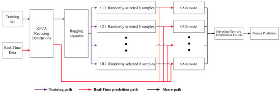
Figure 2.
Principle of KCM–Bagging–GMR.
Step 1: Pre-process the data of training set via standardization;
Step 2: Set the appropriate kernel function parameters and calculate the kernel function matrix in Equation (7) and modify it to get in Equation (8);
Step 3: The eigenvalues of kernel matrix are arranged in descending order;
Step 4: Do the unit orthogonalization of the eigenvector as ;
Step 5: Set the appropriate cumulative contribution threshold and extract the corresponding principal component ;
Step 6: The projection of the kernel matrix on the principal component is calculated, that is , the result after dimensionality reduction is obtained;
Step 7: is randomly sampled B times, and the number of samples selected each time is b;
Step 8: For the new test sample , its output value for the i-th GMR sub-model is calculated;
Step 9: The predicted value of the soft sensor model corresponding to can be obtained from Equation (14);
In order to better evaluate the prediction performance of the model, root mean square error (RMSE) and correlation coefficient (COR) are selected as evaluation indexes, which are defined as
where N is the number of test sample data, is the true value corresponding to the test sample, is the average value of the whole test sample, is the predicted value of the test sample obtained using the model, and is the average value of the predicted value of the test sample. The smaller the value of RMSE is, the higher the accuracy of the established soft measurement model is. The predicted value of the new test point is closer to the true value using the soft sensor model. The closer the value of COR is to 1, the closer the predicted value of the soft sensor model for the new test point is to the true value.
4. Results and Discussion
4.1. Research Object
The ZGM-type medium-speed pulverizer is a commonly used coal grinding equipment in coal-fired power plants. Its working principle involves the following steps: feeding, grinding, classification, and discharge. In the coal-fired power plant, coal is fed into the grinder through the feeding device. Inside the grinder, the coal undergoes grinding and pulverization through the squeezing and grinding action of the roller discs. The roller discs, consisting of multiple rollers with gaps in between, exert pressure on the coal, resulting in its pulverization into fine powder. During the grinding process, the coal is mixed with a certain amount of hot air, which enhances the grinding efficiency and helps remove internal moisture. The ground coal powder, along with the air mixture, enters the classifier where it is classified based on particle size. The classifier separates a portion of the fine powder to be recirculated back to the grinder for secondary grinding, ensuring consistent particle size. Meanwhile, the air containing grinded coal particles is separated and discharged through the exhaust system. The classified fine powder is discharged from the classifier outlet as the final product coal powder. This product is collected and stored using a discharge device for combustion in the boilers. Additionally, the dust generated during the grinding process is collected and treated by the dust collection system to minimize environmental pollution. In summary, the ZGM-type medium-speed grinder in coal-fired power plants operates by grinding coal into fine powder through the squeezing and grinding action of the roller discs. The coal powder is then classified, and the desired particle size is achieved through recirculation and separation. Finally, the collected coal powder is ready for combustion, while the dust is appropriately treated to ensure environmental compliance.
To validate the efficacy of the methodology outlined in this study, pulverization data from a 60 MW power plant are chosen for analysis, accompanied by the selection of 11 auxiliary variables in Table 1. A total of 400 sets of training data are selected, with the main variable being the motor. Out of these, 350 sets are designated as training samples, and the remaining 50 sets are assigned as testing samples. The first step involves standardizing the training samples, followed by dimensionality reduction through KPCA. The Bagging algorithm is then employed to select sub-sample sets, and GMR is utilized to establish individual sub-models. The choice of parameters in the KPCA method significantly impacts the prediction performance. In this study, the model is configured with the following parameters: KPCA parameter is set at 80, with a cumulative contribution rate threshold of 90%. In Bagging coupling with fusion algorithm, B and b are given through a large amount of trial and error, so as to ensure the best accuracy of the calculation. B is set at 5, and b is set at 60%. The modeling process proceeds according to the flowchart outlined in Figure 3, ultimately yielding the final global prediction value.

Table 1.
Auxiliary variable scale for pulverizing.
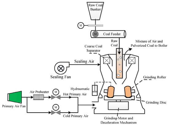
Figure 3.
Structure of ZGM-type medium-speed pulverizer system.
4.2. Simulation Experiment of Pulverizer
In order to further analyze the impact of the data preprocessing methods, Bagging algorithm, and sub-model fusion on the modeling performance, five different methods were simulated and evaluated: KPCA–GMR, PCA–Bagging–GMR, MDS–Bagging–GMR, the proposed KPCA–Bagging–GMR, and the conventional mean fusion [33] approach. MDS, abbreviated for Multidimensional Scaling [29], is an alternative approach to dimensionality reduction. In order to ensure the consistency of comparison conditions, the cumulative contribution thresholds of PCA and MDS are consistent with those of KPCA, which are basically around 90%. These experiments aim to assess the influence of preprocessing methods and fusion techniques on algorithm performance, which run in Python 3.10 environment. Table 2 presents the simulation results of relevant performance metrics.

Table 2.
Performances of different modeling methods.
In Table 2, the results indicate that the proposed KPCA–Bagging–GMR modeling demonstrates the highest predictive accuracy. When compared to the PCA–Bagging–GMR and MDS–Bagging–GMR methods, the utilization of KPCA proves to be more effective in capturing the nonlinear characteristics of the process data. Moreover, in contrast to the KPCA–GMR modeling, it can be observed that the ensemble of multiple models established through the Bagging ensemble learning method effectively enhances the predictive accuracy of the models. Additionally, in comparison to the mean fusion approach, the adoption of the Bayesian fusion technique highlights its ability to better harness the performance of the local models. This ensures that local models with higher predictive performance carry higher weights, thereby maximizing the advantages of ensemble learning.
Figure 4 shows the predictive results obtained using different preprocessing methods, namely PCA, MDS, and KPCA, for constructing soft measurement models. Upon comparing the predictive result graphs of the three methods, it is evident that the overall accuracy of the soft measurement models constructed using nonlinear preprocessing methods is higher. Additionally, the soft measurement model established using the KPCA preprocessing method outperforms the model constructed using MDS. This indicates that the proposed KPCA–Bagging–GMR modeling method exhibits superior predictive accuracy. For processes with strong nonlinearity, KPCA demonstrates a superior ability to handle nonlinear features compared to PCA and MDS. Figure 5 illustrates the relative error results of the soft measurement models constructed using different preprocessing methods, clearly indicating the modeling approach utilizing KPCA preprocessing.
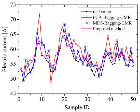
Figure 4.
Prediction of different pretreatment methods.
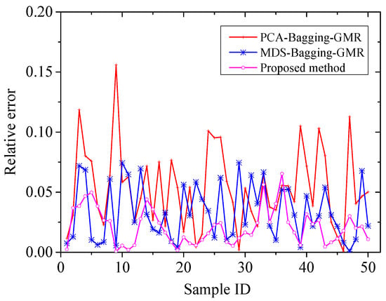
Figure 5.
Relative error of different pretreatment methods.
In Figure 6, the relative error corresponding to different fusion methods employed in the modeling approach is presented. It can be observed from the figure that the proposed method in this study exhibits a lower overall relative error compared to the mean fusion approach. In other words, the predictive accuracy of the Bayesian posterior probability fusion method is higher than that of the conventional mean fusion method. By using the Bayesian posterior probability to compute the weight coefficients of each sub-model, the proposed method effectively enhances the weights corresponding to locally superior models, thereby improving the overall performance of the model.
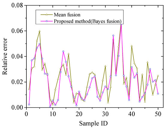
Figure 6.
Relative error of different fusion methods.
5. Conclusions
The nonlinearity, high dimensionality, and time-varying nature of the operational conditions of a pulverizer in power plants bring about difficulties for the data-driven soft sensing modeling. Existing individual models in ensemble learning are rooted in extracting the correlation between the input and output data from the original dataset, which inherently encompasses substantial noisy data. To address this, the present study introduces the KPCA dimensionality reduction technique and extracts distinctive features of the input information for the pulverizer, subsequently establishing an ensemble learning model (Bagging algorithm + Bayesian fusion) that correlates the feature values with the output quantities. Experimental simulations on pulverizer processes demonstrate that the ensemble soft sensing modeling approach based on KPCA effectively predicts the electric current in the pulverizer process, showing superior predictive accuracy and excellent generalization capabilities.
Author Contributions
Conceptual model and simulation, S.J. and Y.D.; funding acquisition and resource administration, F.S.; sample collection and data acquisition, S.R. All authors have read and agreed to the published version of the manuscript.
Funding
This research was funded by the National Natural Science Foundation of China, grant number 51976031, and the Open Foundation of Key Laboratory of Energy Thermal Conversion and Control of Ministry of Education.
Data Availability Statement
The original contributions presented in the study are included in the article, and further inquiries can be directed to the corresponding author.
Acknowledgments
The authors would like to extend their sincere gratitude to the relevant institutions for their financial and technical support.
Conflicts of Interest
The authors declare no conflict of interest.
References
- Eslick, J.C.; Zamarripa, M.A.; Ma, J.; Wang, M.; Bhattacharya, I.; Rychener, B.; Pinkston, P.; Bhattacharyya, D.; Zitney, S.E.; Burgard, A.P.; et al. Predictive Modeling of a Subcritical Pulverized-Coal Power Plant for Optimization: Parameter Estimation, Validation, and Application. Appl. Energy 2022, 319, 119226. [Google Scholar] [CrossRef]
- Saif-ul-Allah, M.W.; Khan, J.; Ahmed, F.; Hussain, A.; Gillani, Z.; Bazmi, A.A.; Khan, A.U. Convolutional Neural Network Approach for Reduction of Nitrogen Oxides Emissions from Pulverized Coal-Fired Boiler in a Power Plant for Sustainable Environment. Comput. Chem. Eng. 2023, 176, 108311. [Google Scholar] [CrossRef]
- Agrawal, V.; Panigrahi, B.K.; Subbarao, P.M.V. Review of Control and Fault Diagnosis Methods Applied to Coal Mills. J. Process Control. 2015, 32, 138–153. [Google Scholar] [CrossRef]
- Hong, X.; Xu, Z.; Zhang, Z. Abnormal Condition Monitoring and Diagnosis for Coal Mills Based on Support Vector Regression. IEEE Access 2019, 7, 170488–170499. [Google Scholar] [CrossRef]
- Xu, W.; Huang, Y.; Song, S.; Cao, G.; Yu, M.; Cheng, H.; Zhu, Z.; Wang, S.; Xu, L.; Li, Q. A Bran-New Performance Evaluation Model of Coal Mill Based on GA-IFCM-IDHGF Method. Meas. J. Int. Meas. Confed. 2022, 195, 126171. [Google Scholar] [CrossRef]
- Banik, R.; Das, P.; Ray, S.; Biswas, A. Wind Power Generation Probabilistic Modeling Using Ensemble Learning Techniques. Mater. Today Proc. 2019, 26, 2157–2162. [Google Scholar] [CrossRef]
- Zhong, X.; Ban, H. Crack Fault Diagnosis of Rotating Machine in Nuclear Power Plant Based on Ensemble Learning. Ann. Nucl. Energy 2022, 168, 108909. [Google Scholar] [CrossRef]
- Wen, X.; Li, K.; Wang, J. NOx Emission Predicting for Coal-Fired Boilers Based on Ensemble Learning Methods and Optimized Base Learners. Energy 2023, 264, 126171. [Google Scholar] [CrossRef]
- Cai, J.; Ma, X.; Li, Q. On-Line Monitoring the Performance of Coal-Fired Power Unit: A Method Based on Support Vector Machine. Appl. Therm. Eng. 2009, 29, 2308–2319. [Google Scholar] [CrossRef]
- Zhang, X.; Zhao, J. Prediction Model for Rotary Kiln Coal Feed Based on Hybrid SVM. Procedia Eng. 2011, 15, 681–687. [Google Scholar] [CrossRef][Green Version]
- Yao, Z.; Romero, C.; Baltrusaitis, J. Combustion Optimization of a Coal-Fired Power Plant Boiler Using Artificial Intelligence Neural Networks. Fuel 2023, 344, 128145. [Google Scholar] [CrossRef]
- Doner, N.; Ciddi, K.; Yalcin, I.B.; Sarivaz, M. Artificial Neural Network Models for Heat Transfer in the Freeboard of a Bubbling Fluidised Bed Combustion System. Case Stud. Therm. Eng. 2023, 49, 103145. [Google Scholar] [CrossRef]
- Yu, Z.; Yousaf, K.; Ahmad, M.; Yousaf, M.; Gao, Q.; Chen, K. Efficient Pyrolysis of Ginkgo Biloba Leaf Residue and Pharmaceutical Sludge (Mixture) with High Production of Clean Energy: Process Optimization by Particle Swarm Optimization and Gradient Boosting Decision Tree Algorithm. Bioresour. Technol. 2020, 304, 123020. [Google Scholar] [CrossRef] [PubMed]
- Cao, H.; Chen, W.; Jia, L.; Zhang, Y.; Lu, Y. Cluster Analysis Based on Attractor Particle Swarm Optimization with Boundary Zoomed for Working Conditions Classification of Power Plant Pulverizing System. Neurocomputing 2013, 117, 54–63. [Google Scholar] [CrossRef]
- Li, X.; Wu, Y.; Chen, H.; Chen, X.; Zhou, Y.; Wu, X.; Chen, L.; Cen, K. Coal Mill Model Considering Heat Transfer Effect on Mass Equations with Estimation of Moisture. J. Process Control. 2021, 104, 178–188. [Google Scholar] [CrossRef]
- Niemczyk, P.; Dimon Bendtsen, J.; Peter Ravn, A.; Andersen, P.; Søndergaard Pedersen, T. Derivation and Validation of a Coal Mill Model for Control. Control. Eng. Pract. 2012, 20, 519–530. [Google Scholar] [CrossRef]
- Dai, Q.; Ye, R.; Liu, Z. Considering Diversity and Accuracy Simultaneously for Ensemble Pruning. Appl. Soft Comput. J. 2017, 58, 75–91. [Google Scholar] [CrossRef]
- Shiue, Y.R.; You, G.R.; Su, C.T.; Chen, H. Balancing Accuracy and Diversity in Ensemble Learning Using a Two-Phase Artificial Bee Colony Approach. Appl. Soft Comput. 2021, 105, 107212. [Google Scholar] [CrossRef]
- Khoder, A.; Dornaika, F. Ensemble Learning via Feature Selection and Multiple Transformed Subsets: Application to Image Classification. Appl. Soft Comput. 2021, 113, 108006. [Google Scholar] [CrossRef]
- Mohammed, A.; Kora, R. A Comprehensive Review on Ensemble Deep Learning: Opportunities and Challenges. J. King Saud Univ.—Comput. Inf. Sci. 2023, 35, 757–774. [Google Scholar] [CrossRef]
- Liu, D.; Shang, J.; Chen, M. Principal Component Analysis-Based Ensemble Detector for Incipient Faults in Dynamic Processes. IEEE Trans. Ind. Inform. 2021, 17, 5391–5401. [Google Scholar] [CrossRef]
- Lu, H.; Su, H.; Zheng, P.; Gao, Y.; Du, Q. Weighted Residual Dynamic Ensemble Learning for Hyperspectral Image Classification. IEEE J. Sel. Top. Appl. Earth Obs. Remote Sens. 2022, 15, 6912–6927. [Google Scholar] [CrossRef]
- Feng, Y.; Wang, X.; Zhang, J. A Heterogeneous Ensemble Learning Method for Neuroblastoma Survival Prediction. IEEE J. Biomed. Health Inform. 2022, 26, 1472–1483. [Google Scholar] [CrossRef]
- Farrell, A.; Wang, G.; Rush, S.A.; Martin, J.A.; Belant, J.L.; Butler, A.B.; Godwin, D. Machine Learning of Large-Scale Spatial Distributions of Wild Turkeys with High-Dimensional Environmental Data. Ecol. Evol. 2019, 9, 5938–5949. [Google Scholar] [CrossRef] [PubMed]
- Kuang, F.; Xu, W.; Zhang, S. A Novel Hybrid KPCA and SVM with GA Model for Intrusion Detection. Appl. Soft Comput. J. 2014, 18, 178–184. [Google Scholar] [CrossRef]
- Cao, L.J.; Chua, K.S.; Chong, W.K.; Lee, H.P.; Gu, Q.M. A Comparison of PCA, KPCA and ICA for Dimensionality Reduction in Support Vector Machine. Neurocomputing 2003, 55, 321–336. [Google Scholar] [CrossRef]
- Zhao, Y.; Zhou, M.; Xu, X.; Zhang, N. Fault Diagnosis of Rolling Bearings with Noise Signal Based on Modified Kernel Principal Component Analysis and DC-ResNet. CAAI Trans. Intell. Technol. 2023, 8, 1014–1028. [Google Scholar] [CrossRef]
- Sha, X.; Diao, N. Robust Kernel Principal Component Analysis and Its Application in Blockage Detection at the Turn of Conveyor Belt. Measurement 2023, 206, 112283. [Google Scholar] [CrossRef]
- Liu, Z.; Han, H.G.; Dong, L.X.; Yang, H.Y.; Qiao, J.F. Intelligent Decision Method of Sludge Bulking Using Recursive Kernel Principal Component Analysis and Bayesian Network. Control. Eng. Pract. 2022, 121, 105038. [Google Scholar] [CrossRef]
- Breiman, L. Bagging Predictors. Mach. Learn. 1996, 24, 123–140. [Google Scholar] [CrossRef]
- Sheng, H.; Xiao, J.; Wang, P. Lithium Iron Phosphate Battery Electric Vehicle State-of-Charge Estimation Based on Evolutionary Gaussian Mixture Regression. IEEE Trans. Ind. Electron. 2017, 64, 544–551. [Google Scholar] [CrossRef]
- Wang, Y.; Liu, Y. Bayesian Entropy Network for Fusion of Different Types of Information. Reliab. Eng. Syst. Saf. 2020, 195, 106747. [Google Scholar] [CrossRef]
- Singh, P.; Bose, S.S. Ambiguous D-Means Fusion Clustering Algorithm Based on Ambiguous Set Theory: Special Application in Clustering of CT Scan Images of COVID-19. Knowl-Based Syst. 2021, 231, 107432. [Google Scholar] [CrossRef]
Disclaimer/Publisher’s Note: The statements, opinions and data contained in all publications are solely those of the individual author(s) and contributor(s) and not of MDPI and/or the editor(s). MDPI and/or the editor(s) disclaim responsibility for any injury to people or property resulting from any ideas, methods, instructions or products referred to in the content. |
© 2023 by the authors. Licensee MDPI, Basel, Switzerland. This article is an open access article distributed under the terms and conditions of the Creative Commons Attribution (CC BY) license (https://creativecommons.org/licenses/by/4.0/).