Article

Risk Assessment of Power Supply Security Considering Optimal Load Shedding in Extreme Precipitation Scenarios

1
Jiaxing Power Supply Company of State Grid, Jiaxing 314000, China
2
Jiaxing Heng-Chuang Electric Power Group Limited Bochuang Materials Branch, Jiaxing 314000, China
3
School of Information Engineering, Zhejiang University of Technology, Hangzhou 310023, China
*
Author to whom correspondence should be addressed.
Energies 2023, 16(18), 6660; https://doi.org/10.3390/en16186660
Submission received: 25 July 2023 / Revised: 5 September 2023 / Accepted: 12 September 2023 / Published: 17 September 2023
(This article belongs to the Section D: Energy Storage and Application)

Abstract

:
Extreme rainfall may induce flooding failures of electricity facilities, which poses power systems in a risk of power supply interruption. To quantitatively estimate the risk of power system operation under extreme rainfall, a multi-scenario stochastic risk assessment method was proposed. First, a scenario generation scheme considering waterlogged faults of power facilities was constructed based on the storm water management model (SWMM) and the extreme learning machine method. These scenarios were merged with several typical scenario sets for further processing. The outage of power facilities will induce power flow transfer which may consequently lead to transmission lines’ thermal limit violation. Semi-invariant and Gram–Charlier level expansion methods were adopted to analytically depict the probability density function and cumulative probability function of each line’s power flow. The optimal solution was performed by a particle swarm algorithm to obtain proper load curtailment at each bus, and consequently, the violation probability of line thermal violations can be controlled within an allowable range. The volume of load curtailment as well as their importance were considered to quantitatively assess the risk of power supply security under extreme precipitation scenarios. The effectiveness of the proposed method was verified in case studies based on the Southeast Australia Power System. Simulation results indicated that the risk of load shedding in extreme precipitation scenarios can be quantitatively estimated, and the overload probability of lines can be controlled within the allowable range through the proposed optimal load shedding scheme.

1. Introduction

With global warming in recent years, extreme natural disasters have occurred frequently [1,2,3]. This has led to a rising level of damage to power systems and induced huge economic losses [4,5,6]. Hereinto, extreme rainfall events have been reported more and more often in recent years, which consequently challenge the safe operation of power systems. For example, the extraordinarily heavy rainfall disaster in Zhengzhou, China, in July 2021 led to waterlogged failures of 13% of the total number of substations, as well as outage events of 2935—220 kV transmission lines and 47,910 kV distribution lines. As a result, 1263 communities, 1,266,300 households, and 89 important users lost power supply. The power system is extremely vulnerable to extreme rainfall. Therefore, it is important to assess the operational risk of power systems and take proper measurements under extreme rainfall.
The operation of a power system is affected by a variety of factors, including stochastic load changes and equipment failures. To properly address the randomness in power systems, risk assessment is one of the promising ways to quantitatively indicate the operation states so effective measures can be accordingly taken to guarantee system security. To consider the adverse impact caused by random lightning on transmission lines, one study [7] proposed a risk assessment method based on multidimensional correlation information fusion. Another study [8] designed a grid risk assessment method on the basis of an evolutionary strategy and a projection tracing algorithm for power system ice-cover hazards. Other literature [9,10,11] has considered risk events of different extreme conditions such as typhoons, mountain fires, and earthquakes in power system operation. Through the probabilistic power flow calculation, the power flow distribution of the power system in different situations can be obtained. These results can be used to assess the reliability and security of the system, and to identify possible risks and potential problems [12]. One study [13] proposed a probabilistic optimal power flow (P-OPF) method in a power system with a high proportion of wind power generation and large load fluctuations by considering the correlation of variables in the power grid. Another study [14] proposed a probabilistic power flow calculation method with kernel density estimation, which reduced the error in the linearization process as well as calculation burden; [15] established a multi-scenario algorithm to overcome the limitations of semi-invariance in stochastic power flow model with high percentage of renewable energy in power systems. Based on Gram–Charlier level expansion method, a different study [16] calculated the power system violation probability, providing an effective method to find weak links of the power system. Another study [17] developed a risk model to assess grid operation states under different weather conditions through multi-objective particle swarm algorithm and fuzzy set theory, which provides helpful indicators for optimal risk dispatch; [18] simplified the computational process by transforming the constrained optimization model into an unconstrained model through the penalty function on the basis of an improved particle swarm algorithm.
With the change of climate, extreme events will happen more often than before. Extreme precipitation may lead to waterlogging in low-lying areas. The topography around power facilities such as substations built in early years has changed considerably with the development of cities, and many of them are prone to flooding under extreme precipitation conditions which, in turn, leads to flooding outage accidents and even cascading failures of power systems in serious cases. Power system emergencies can lead to losses in various load categories [19]. The analysis using AHP [20] (analytic hierarchy process) and ANP [21] (analytic network process) allows for a comprehensive assessment of different load buses, considering their respective social, economic, and political importance.
To address this problem, this paper proposes a probabilistic power flow-based risk assessment method to quantitatively indicate system operation states under extreme precipitation conditions. The storm water management model (SWMM) was adopted to establish the relationship between rainfall capacity and water levels of specific areas, and the machine learning algorithm finally output the operation state of a power facility considering waterlogging risk. On this basis, a probabilistic power flow method based on semi-invariance and Gram–Charlier level expansion was developed to depict the violation probability of transmission line power flow when load transfer is induced by power facility outage. The violation probability was controlled under an allowable value through proper load curtailment schemes. Finally, the risk of power supply security was assessed considering variable importance of different types of loads. The evaluation results obtained in this paper provide effective indicators for power system operators to make correct dispatch decisions under extreme weather conditions of heavy precipitation.

2. Risk Analysis Framework Considering Waterlogged Failures

Extreme precipitation that may lead to waterlogging-caused power facility failures significantly challenges the operation of power systems. In order to quantitatively indicate the operation risk of power systems and take corresponding measurements under extreme precipitation conditions, the main contents of this paper are as follows:
  • Typical fault scenario generation under extreme rainfall
Using historical rainfall data as input, the SWMM [22] model and the data model of the extreme learning machine (ELM) [23] can be used to calculate the curve depicting the change in water accumulation within a specific area under a precipitation intensity curve. To determine the probabilities of different power facility failure scenarios, the Monte Carlo sampling method was employed. The initial scenarios were then refined based on statistical theory to obtain a representative set of typical scenarios.
2.
Stochastic power flow calculation taking into account load uncertainty
Performing random power flow calculations that account for load uncertainty in each typical scenario set. By considering the proportion of different initial fault scenarios within the same typical scenario set, the probability distribution of line power flow was determined using a combination of the semi-invariant and Gram–Charlier series expansion method. The full probability formula was then utilized to derive the probability distribution of the power grid under each typical scenario set as well as the comprehensive scenario.
3.
Optimal load curtailment calculation based on particle swarm algorithm
Once the probability distribution for the comprehensive scenario was obtained, the probability of overloading was calculated for each branch power. This probability of overloading was then used as a constraint in the optimal load curtailment model. The objective function of this model was to minimize the expected load curtailment for each typical scenario. To solve this optimization problem, the particle swarm algorithm was applied. By using the particle swarm algorithm, the optimal load curtailment scheme was determined, which minimizes the expected load curtailment across all typical scenarios.

3. Generation of Typical Fault Scenarios for Power Facilities under Extreme Rainfall

This section mainly introduces three parts: the failure model of electric facilities driven by the combination of knowledge and data, the generation of initial scenario library, and the construction of typical scenarios.

3.1. Power Facility Failure Model

Knowledge-data hybrid-driven algorithms take advantage of physics-based knowledge models and data-driven machine learning methods to improve the accuracy and reliability of the obtained models. In the power facility fault model presented in this paper, the weight parameters of the extreme learning machine neural network were trained using data such as atmospheric circulation mode, air pressure distribution, and wind speed as input. The data source was the China Statistical Yearbook [24] and the Sigmoid function was used as the activation function This trained network was then employed to predict future rainfall intensity. Based on these predictions, the SWMM model was used to calculate the water depth changes in a specific area. Taking into account factors such as rainfall loss and confluence, a flood failure model for power facilities in the area was established.
The training process of ELM involved the following steps: for a given training dataset, we began by randomly initializing a weight matrix that connected the input layer to the hidden layer. Next, the input data were mapped to the hidden layer through matrix operations. The calculation of the hidden layer output matrix is as follows:
H = g ( X * W + b )
where H is the output matrix of the hidden layer, g ( · ) is the activation function, its input matrix is X , and the weight matrix between the input layer and the hidden layer is W , and the bias vector is b . On this basis, a linear model was built between the nodes of the hidden layer and the nodes of the output layer, and the weight matrix of the linear model is solved, which is calculated as follows:
β = p i n v ( H ) * y h
where β is the output layer weight matrix, p i n v ( H ) denotes the generalized inverse matrix H , and y h is the expected output matrix. The resulting weight matrix is applied to the test data for prediction which is calculated as follows:
y = g ( X * W + b ) * β
where y is the output of the extreme learning machine, namely the prediction of rainfall intensity.
The extreme learning machine (ELM) component is comprised of three main parts: the input layer, the hidden layer, and the output layer. This structure is depicted in the upper section of Figure 1. Additionally, the lower section of Figure 1 illustrates the process of constructing a mapping model between rainfall intensity and ponding depth using the SWMM model. This model is built based on the rainfall intensity curve generated by the ELM. In summary, the lower part of the figure demonstrates how the SWMM model leverages the rainfall intensity curve produced by the ELM to establish a mapping model for rainfall intensity and water depth.
According to the extreme learning machine method mentioned above, the predicted rainfall intensity was obtained, and the input of it as the SWMM model was further established to create a mapping model between rainfall and water depth. The model enables the identification of flooding fault scenarios and their associated probabilities in a specific area. It analyzed the rainfall patterns across different regions, distinguishing between pervious and impervious areas, as well as regions with and without depressions [25]. These distinctions account for various forms of rainfall loss, such as evaporation during the rainy season (applicable to both pervious and impervious regions), depression (relevant for impervious areas with depressions), and permeable runoff (pertaining to permeable areas). The surface runoff flow was calculated by subtracting these three components from the total rainfall [26]. The mathematical expression is as follows:
I = Q q i q e D
where I denotes the surface runoff flow, Q denotes the rainfall intensity, q i denotes infiltration rainfall, q e denotes evaporation of rainwater (generally not considered), and D is the amount of water of low-lying land. It is worth noting that the output of the extreme learning machine y will be substituted into Q in order to calculate the surface runoff flow through Equation (4).
The calculation formula of the infiltration part loss in this area is as follows (the infiltration part is calculated using the Horton infiltration model [27]):
q i = I t * S t * t
i t = f 1 + ( f 0 f 1 ) e a t
In Equations (5) and (6), I t is the average seepage rate in the t time period, t is any time interval, S t is the area of each permeable zone, f 0 is the initial infiltration rate, f 1 is the final infiltration rate, and a is the decreasing infiltration rate.
After accounting for the rainfall loss, the model focuses on studying the confluence component to calculate the ponding depth in the relevant area. The confluence component is further divided into two parts: surface confluence and pipeline network confluence. The confluence of the pipeline network refers to the water discharged through the pipeline via the basin outlet. It represents the portion of water flow managed by the drainage system.
The flow rate of the pipeline network was determined by the drainage capacity and drainage time of the network. This capacity indicates the amount of water that can be effectively discharged through the pipeline system within a given period.
The calculation formula is as follows:
Q p = 1 n π d r 2 4 ( d r 4 ) 2 3 S p 1 2 Δ t
where Q p is the sink flow of the pipe network, n is the inner wall of water pipe roughness, d r is the pipe diameter, S p is the slope of the bottom of the pipe, and Δ t is the drainage calendar time.
The surface flow process can be effectively modeled by considering the catchment as a nonlinear reservoir. In this modeling approach, the catchment area is taken into account, and the flow rate is used as an input to the model. By analyzing the relationship between the outflow rate at the basin outlet and the water depth, a nonlinear function describing this relationship can be derived. The nonlinear reservoir model is calculated as follows:
d V d t = S d d d t = S i Q c
Q c = W f l 1.49 n ( d d p ) 5 3 S l 1 2
In Equations (8) and (9), V is the water volume in catchment area V = s * d ;  d is the nodal corresponding water depth; S is the area of the catchment area; i is the produced flow calculated by the previous part; Q c is the outflow; W f l is the diffuse width of the catchment area [28], meaning the distance that the fluid expands horizontally on the bed in a region with uneven topography; n is the surface Manning roughness coefficient whose value differs significantly between permeable and impermeable areas; d p is the surface stagnant water depth whose value was obtained by analyzing the land elevation data; and S l is the slope of the catchment area. Combining Equations (8) and (9), d and Q c can be obtained. After considering the prediction error (error calculation is explained in Section 3.2), the predicted ponding depth of the corresponding node of the power facility was obtained. When the predicted water level is greater than or equal to the height of the substation, it is considered that a risk event occurs.
The initial scenario of water immersion failure was generated using a non-sequential Monte Carlo sampling method, which allows for the generation of diverse and representative scenarios. This process involves randomly sampling from a range of possible inputs to obtain a set of initial fault scenarios. The corresponding probabilities of these scenarios were then calculated. The generation process for the initial fault scenarios in the power system is presented in Algorithm 1.
Algorithm 1. Electric utility failure scenario generation process.
Input :   past   storm   curve   data   X i   activation   function   g ( · ) ,   number   of   hidden   layer   neurons   K ;
Output: probability of failure of electrical facilities
1: Import   a   rainfall   dataset   as   input ,   noted   as   storm   curve   data   X i ;
2: Data   preprocessing :   processing   of   the   desired   output   into   a   row   vector ,   where   each   element   of   the   vector   represents   a   category ,   and   calculation   of   the   desired   output   matrix   y h ;
3: Set   the   activation   function   g ( · ) ,   the   number   of   hidden   layer   neurons   K ,   and   randomly   initialize   the   weight   matrix   W   and   the   bias   vector   b between the input layer and the hidden layer, where the weights are randomly generated between [−1,1] and the connection bias is randomly generated between [0,1];
4: Calculate   the   hidden   layer   output   matrix   according   to   Equation   ( 1 ) ,   where   X is the matrix with each element being past storm curve data
5:Calculate the output layer weight matrix according to Equation (2);
6:Calculation of the output prediction data and visualization of the rainfall curve according to Equation (3);
7: Calculate   the   amount   of   infiltration   q i according to Equations (5) and (6);
8:Enter the puddle storage and evaporation volumes and calculate the production flow according to Equation (4);
9: Calculate   the   pipe   network   sin k   flow   rate   Q p according to Equation (7);
10:Calculate the variation curve of the ponded water level with time for a given precipitation intensity profile for the power facility according to Equations (8) and (9).

3.2. Generate the Initial Set of Scenarios

Based on the previous section’s introduction, a water depth curve over time can be calculated for a specific area based on the predicted values of the rainfall intensity curve. However, it is important to consider that there may be some errors in the prediction of rainfall intensity. These errors can arise due to the inherent randomness in historical data, potentially leading to data quality issues. In this paper, it was assumed that the fluctuation between the actual rainfall intensity and the predicted value follows a normal distribution. The amplitude of the error fluctuation curve was considered to conform to a 3σ normal distribution, with the expected value corresponding to the intensity of the predicted rainfall at that moment. The expression of the error value is shown in Equation (10):
f x ; μ ; σ = 1 2 π σ * exp ( ( x μ ) 2 2 σ 2 )
where x is the prediction error value, μ is the predicted rainfall intensity value, and σ is the mathematical variance. A normal random number, also known as a Gaussian random number, is a number generated from a normal distribution. In a normal distribution, the probability of occurrence is highest around the mean (expectation) value and decreases as the number deviates from the mean, the standard deviation is assumed to be 10% of the average value.
To determine the operational status of the substation, suppose there are n substations in a power grid, and the state probability characteristics of each substation are described by a random number that obeys the 0–1 distribution [29], and each substation has only two states of normal and fault where normal corresponds to 1, fault corresponds to 0, and whether different substations are faulty is independent of each other. The substation number is denoted as k , S k indicating the operating state of the substation k , and the grid operating state (denoted as S ) is composed of the states of each substation in the grid. Therefore, the operating state of the grid can be expressed as S = ( S 1 , S 2 , , S n ) , which means the initial fault scenario of the power facility is obtained.
The final water depth value is obtained by taking into account both the calculation method and the prediction error of the water accumulation height, as proposed in the previous section. By comparing this final water depth value with the height of the substation, the operational status of the substation can be determined.
This approach ensures a comprehensive evaluation of the water accumulation height, considering both the calculated value and the potential prediction errors. The height of multiple substations in the order of H 1 , H 2 , ,   H n . The substation status is determined according to the following equation:
S k = 0       d t H k 1       d t < H k
where S k is the state of the substation k , H k is the state of the substation k , and d t represents the ponding depth at the moment   t . The sampling process is shown in Figure 2. It is worth noting that the probability of 0 or 1 will be changed as the variation of the rainfall curve in different time period as well as the topography of different places.

3.3. Building Typical Scenario Sets

Once the initial library of failure scenarios is generated, the scenarios whose occurrence probability is significantly lower than the others are ignored according to statistical principles. The resulting typical scenario set fully represents the possible fault scenarios in reality and provides more scientific guidance for the safe and stable operation of the power system. Through the setting of typical scenarios, more specific and targeted preventive measures can be implemented for different fault scenarios, effectively reducing losses caused by risk events. In addition, the typical scenario set has important reference value for the formulation of emergency plans. By considering different failure scenarios, corresponding contingency plans can be developed in advance, ensuring the proper configuration of personnel and equipment to respond quickly and efficiently in the event of a failure.
In summary, the generation of a typical scenario set offers practical benefits for power system operations. It allows for tailored preventive measures, minimizes losses resulting from risk events, and aids in the formulation of proactive emergency plans. This comprehensive approach enhances the overall resilience and reliability of the power system.

4. Stochastic Power Flow Calculation Considering Load Uncertainty

4.1. Calculation of Semi-Invariance of Each Order in a Typical Scenario

The typical outage scenarios of each power facility generated above is defined as T j . The probability density function f j ( x ) and cumulative distribution function F j ( x ) of the power system state quantity x considering the load uncertainty under Scenario a can be obtained by semi-invariant method and the Gram–Charlier series expansion method.
Prior to calculating the semi-invariants of each order for each random variable, it is essential to conduct deterministic power flow calculations. These calculations are performed to determine the reference operating point of the power grid. On this basis, the bus voltage state variable Δ X and the branch power flow state variable Δ Z can be further obtained according to the random distribution of the load, and the Jacobian matrix J 0 (Power System Jacobian Matrix) and sensitivity matrix S 0 can be calculated. The nodal and branch equations of the power system are expressed as shown in Equations (12) and (13) after carrying out Taylor series expansion at the base operating point and neglecting the higher terms of 2 or more times.
W = W 0 + Δ W = f X = f X 0 + Δ X f X 0 + J 0 * Δ X
Z = Z 0 + Δ Z = g X = g X 0 + Δ X g X 0 + G 0 * Δ X
In Equations (12) and (13), W is bus injection variable, X is bus state variables, Z is branch state variables, and J 0 = f ( X ) X X = X 0 , G 0 = g ( X ) X X = X 0 .
The following equation conditions are satisfied at the reference operating point of the power grid.
W 0 = f X 0 Z 0 = g X 0
Then, the linearization equation for the random perturbation Δ W at the reference operating point of the power grid can be obtained. The linearized equation is shown in Equation (15):
Δ X = J 0 ( 1 ) Δ W = S 0 Δ W Δ Z = G 0 S 0 Δ W = T 0 Δ W
According to the homogeneity and additivity of the semi-invariant [30] and the relationship between the power system bus injection quantity and the state quantity in Formula (15), half of the system state quantity can be obtained according to the semi-invariant of the bus injection variable invariant.

4.2. Gram-Charlier Series Expansion Method

Based on the semi-invariants of each order for each random variable, the probability density function and cumulative distribution function of each random variable can be determined using the Gram–Charlier series expansion method. The Gram–Charlier series expansion method allows for expanding the distribution function of a random variable into a series consisting of derivatives of each order of the normal random variable. The coefficients of the series can be expressed as the semi-invariants of each order of the random variable [31]:
g v = γ v δ v = γ v γ 2 v / 2
where γ v is called the v order normalized semi-invariant and is also the coefficient in each expansion of the Gram–Charlier series, and δ is the standard deviation.
Let F ( x ) and f ( x ) be the cumulative distribution function and the probability density function of the standardized random variable x , respectively, the f ( x ) is the derivative of F ( x ) . The Gram–Charlier series expansions of F ( x ) and f ( x ) are of the following form [31]:
F ( x ) = x φ ( x ) d x + φ ( x ) [ g 3 3 ! H 2 ( x ) + g 4 4 ! H 3 ( x ) + g 5 5 ! H 4 ( x ) + ]
f ( x ) = φ ( x ) [ 1 + g 3 3 ! H 3 ( x ) + g 4 4 ! H 4 ( x ) + g 5 5 ! H 5 ( x ) + ]
In Equations (17) and (18), φ ( x ) is the probability density function of the standard normal distribution, and H v ( x ) denotes the Hermite polynomial of v order Hermite polynomials are a set of orthogonal polynomials, which are usually used to deal with problems related to quantum mechanics, mathematical physics, and probability theory.
In summary, based on the semi-invariant and Gram–Charlier series expansion, the stochastic power flow algorithm process is shown in Figure 3:
In Figure 3, after the reference operating point is calculated, the node injection variable Δ W is obtained according to the load fluctuation, the sensitivity matrix S 0 and the transfer matrix T 0 are obtained after constructing the Jacobian matrix, and then the probability density function and cumulative distribution function of different initial fault scenarios are obtained. Next, the corresponding results for each typical set of scenarios and synthetic scenarios are calculated using the total probability formula. A more comprehensive understanding of system performance can be obtained by employing a fully probabilistic formulation and considering the collective impact of multiple scenarios.
f ( x ) = j = 1 n p j f j ( x ) F ( x ) = j = 1 n p j F j ( x )
In Equation (19), p j is the probability of occurrence of typical scenario j , and f j ( x ) and F j ( x ) are the calculation results of the probability distribution of variable x in scenario j respectively.

5. Particle Swarm Algorithm-Based Decision Model for Load Curtailment Optimization

5.1. Optimal Load Curtailment Model

During the operation of power systems, various risk events can occur as a result of power facility failures and load fluctuations. In order to address this challenge, this paper presents a nodal load curtailment optimization model based on stochastic power flow. The proposed model ensures the power balance of the system while preventing branch power flows from exceeding their limits. By optimizing the load curtailment at each bus, the model aims to minimize the risk of power system failures and maintain stable operations. The objective function of the optimization model is formulated as the product of the probability of occurrence under a typical scenario set and the minimum expected reduction in bus load under different scenario sets. Mathematically, the bus load curtailment optimization model can be represented as follows:
E a l l = m i n s e N S P s e j J α j i N D C i
where E a l l is the expected sum of load curtailment for all typical scenario sets, N S is the number of typical scenario sets obtained by statistical methods, P s e is the probability of occurrence of any typical scenario set, α j is the weighting factor used to indicate the types of different buses, J is the number of types of different buses, C i is the load curtailment on bus i , and N D is the set of load buses.
Constraints:
0 C i P D i ( i N D )
The physical meaning of Equation (21) is that the amount of curtailment of load on bus i cannot be greater than the rated load on bus i .
F T k S T k m a x 0.05
In Equation (22), T k m a x is the value of the volt-amperes tidal current withstood on line k . T k ( S ) is the rated transmitted power on line k . F T k S is the tidal current crossing probability of each branch.

5.2. Particle Swarm Algorithm-Based Solution Process

Particle swarm optimization (PSO) [32] is an optimization algorithm inspired by the foraging behavior of birds. In PSO, candidate solutions are represented as a group of particles, with each particle representing a potential solution in the search space. These particles iteratively update their positions and velocities based on individual and group experiences, aiming to converge towards the optimal solution.
The algorithm involves several key factors, including acceleration factors c 1 and c 2 , and the inertia factor ω . These factors influence the speed at which particles move towards their individual optimal positions and the global optimal position, balancing exploration and exploitation. In this paper, an improved particle swarm algorithm was employed to calculate the objective function. To ensure the feasibility of the solutions, a constraint function was added to the original objective function as a penalty function. This penalty function guides the iterative process to approach the feasible region of the solution space, encouraging the particles to converge towards viable solutions. By integrating these enhancements into the particle swarm optimization framework, the algorithm in this paper can effectively search for optimal solutions while satisfying the specified constraints. The solution formula of the penalty function is explained as Formula (23):
F ( x , M ) = f ( x ) + M p ( x )
where f ( x ) is the objective function and M p ( x ) is the penalty term. The penalty factor M is a sufficiently large real number, and the optimal solution of F ( x , M ) is close to the optimal solution of the constrained problem.

6. Example Analysis

In this paper, the South East Australian Power System [33] was used as an example for simulation purposes. The buses in the system were categorized into three classes: buses 1–6 were classified as Class I loads with a weight factor α 1 of 0.5, buses 7–12 were designated as Class II loads with a weight factor α 2   of 0.3, and buses 13–17 were categorized as Class III loads with a weight factor α 3 of 0.2. To model load fluctuations, numerous relevant literature sources indicate that these fluctuations follow a normal distribution pattern. Therefore, it is assumed in this study that the load fluctuations at each bus conform to a normal distribution. The expected value of the load fluctuation was set as the rated value of the respective bus load, and the standard deviation was assumed to be 20% of the average value. After inputting the training set data mentioned above, the root-mean-square error (RMSE) of rainfall intensity between the predicted result obtained by using the extreme learning machine and the actual one was 0.0492.
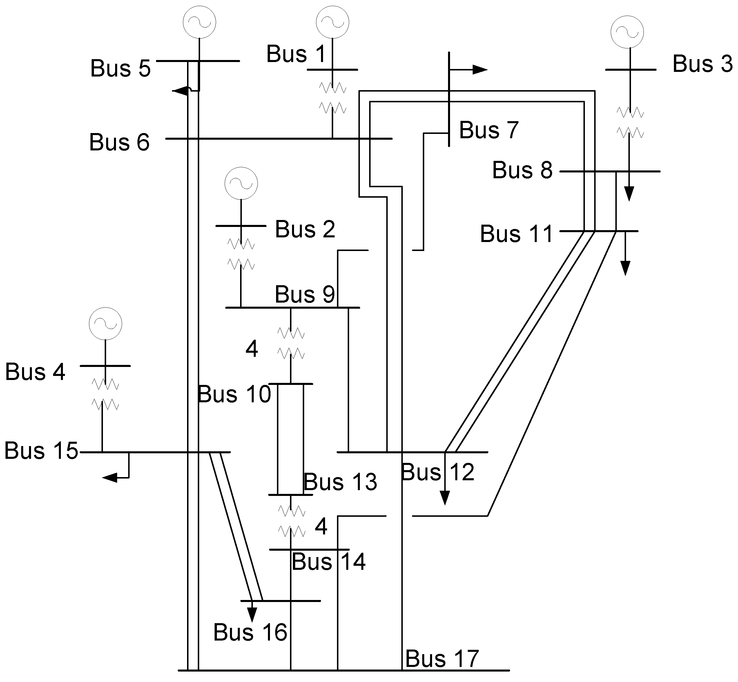
The network topology of the power system is illustrated in Figure 4.

6.1. Typical Scenario Generation

6.1.1. Outage Scenario Generation Model

Table 1 presents the relevant data necessary for the fault scenario generation model of power facilities proposed in this study. This dataset includes essential information required for the analysis and assessment of power system faults.

6.1.2. Rainfall and Water Distribution

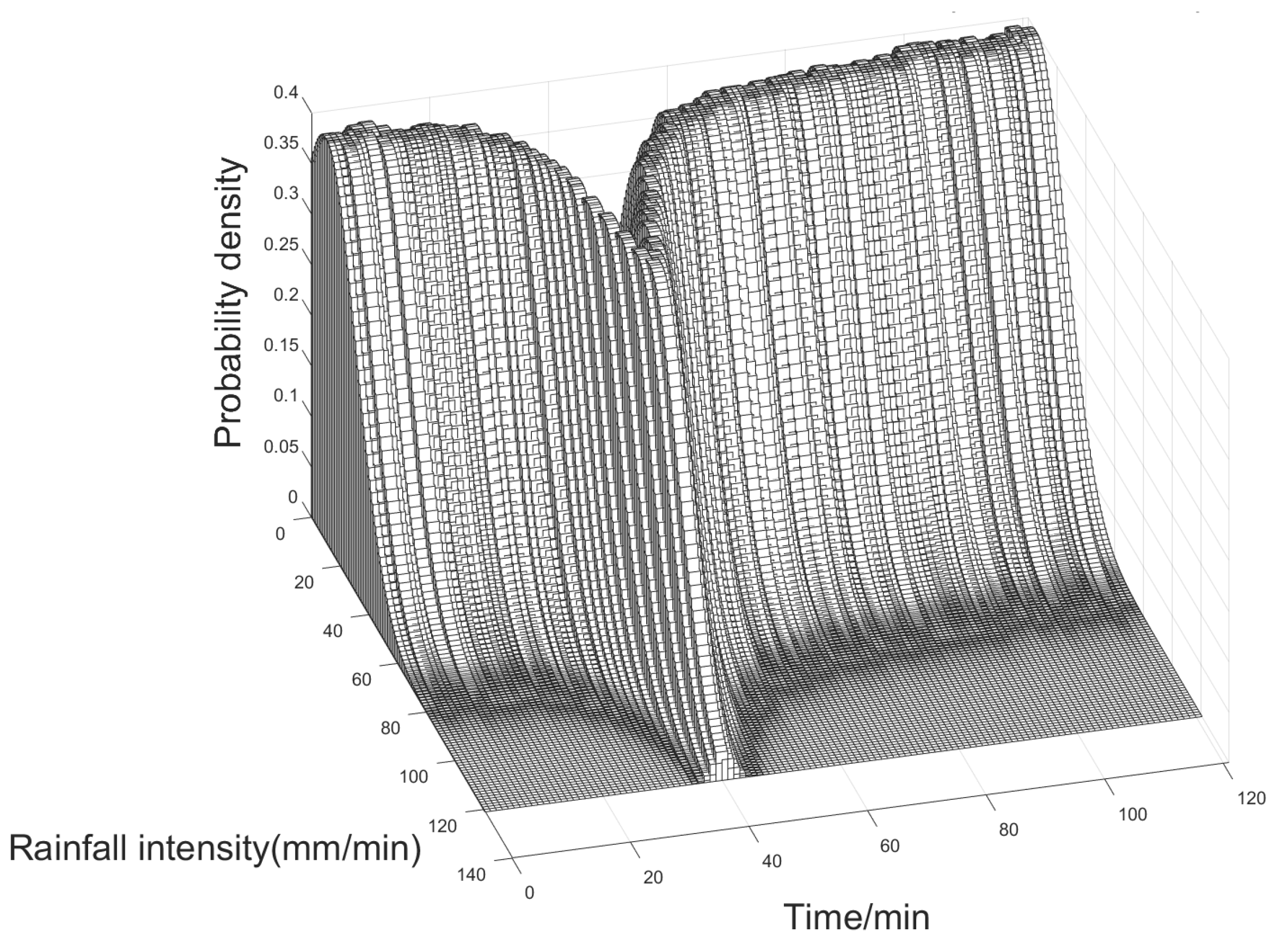
Assuming that the rainfall intensity follows a standard normal distribution, Figure 5 presents a three-dimensional plot showcasing the relationship between time, rainfall intensity, and the corresponding probability density. In the plot, the X-axis represents time in minutes, the Y-axis represents the instantaneous rainfall intensity in millimeters per minute (mm/min), and the Z-axis represents the probability density associated with the instantaneous rainfall intensity at a given time.
Figure 5 depicts the fluctuation of rainfall intensity within a specific range over time. It is observed that the rainfall intensity varies within certain bounds, exhibiting temporal variations. The probability density initially increases and then decreases as time elapses. As time advances, the probability density distribution reflects the changing likelihood of different rainfall intensity values. Moreover, it is apparent from the plot that when the rainfall intensity is large, the corresponding probability density tends to be smaller. This suggests that extreme rainfall events, characterized by higher intensities, occur with lower probabilities compared to moderate or lower intensity rainfall.
The observations derived from Figure 6 offer valuable information about the probabilistic characteristics of water depth over time. It is apparent that the probability density decreases as water depth increases during the first half of the time period. Moreover, in the second half of the time, the rate at which water depth increases, corresponding to higher probability density, gradually slows down. This suggests that as water depth reaches higher levels, the likelihood of further significant increases diminishes.

6.1.3. Scenario Library Generation and Reduction

After obtaining the distribution of rainfall intensity, the power system outage scenarios and their respective probabilities were determined using Monte Carlo sampling, as illustrated in Figure 7. The sampling was performed 10,000 times to capture a comprehensive range of possible scenarios. In the power system under consideration, the influence of the failure of two internal substations (namely 9–10, 13–14) on the power system was studied. There were four transformers in each of the two substations, and their heights were 0.9 m, 0.85 m, 0.8 m, and 0.75 m.
The bar chart presented in Figure 7 displays the results after applying statistical theory to discard low probability events. In this chart, (a), (b), and (c) represent the probabilities of occurrence for the same initial failure scenario under different conditions. The typical scenarios depicted in the bar chart are differentiated based on the number of faults occurring in the substations. Each bar represents a specific scenario, and its height corresponds to the probability of that scenario occurring. This approach ensures that the subsequent analysis and decision-making processes are based on typical scenarios that possess higher probabilities of occurrence.

6.2. Curtailment of Load Simulation Results

To validate the efficacy of the proposed method, the benchmark value was defined as the power capacity that each branch can withstand under normal operating conditions. In this context, the power of 1.2 times the normal operating level was set as the limit for overloading. Table 2 provides the values of the power capacity for each branch under normal operating conditions.
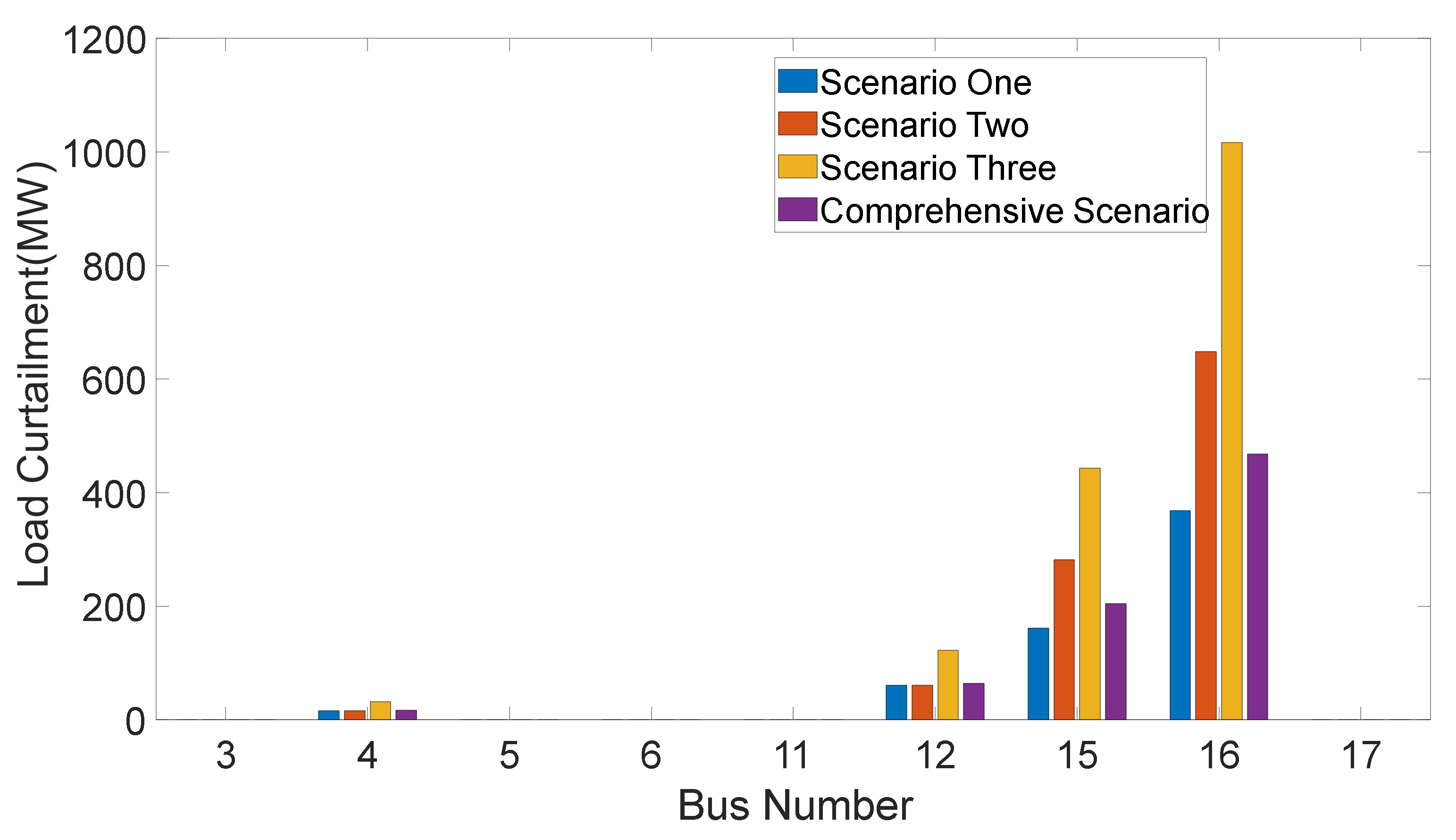
Table 3 lists the total grid load reduction for each typical scenario group. It shows the cumulative load shedding, taking into account power system load fluctuations under various conditions. It was found through analysis that the total load shedding of all buses in the power system increased with the number of substation faults. This indicates that as the number of substation failures increases, more loads need to be shed to maintain power system stability and avoid overloading.
Figure 8 illustrates the load curtailment at the main buses for each typical scenario set and the comprehensive scenario. It is important to note that the load curtailment amounts at other buses, which are not depicted in the figure, are considerably smaller compared to the buses displayed. The focus of Figure 8 is on showcasing the load curtailment levels at the main buses that are most significantly impacted by the identified scenarios. These buses are typically the ones experiencing the highest load curtailment requirements and, therefore, require particular attention in terms of load management strategies and contingency planning.

6.3. Simulation Results of Branch Power Flow Violation

Branches (9–10, 13–14) were designated as failure setpoints in the analysis. There were four transformer groups in each substation.
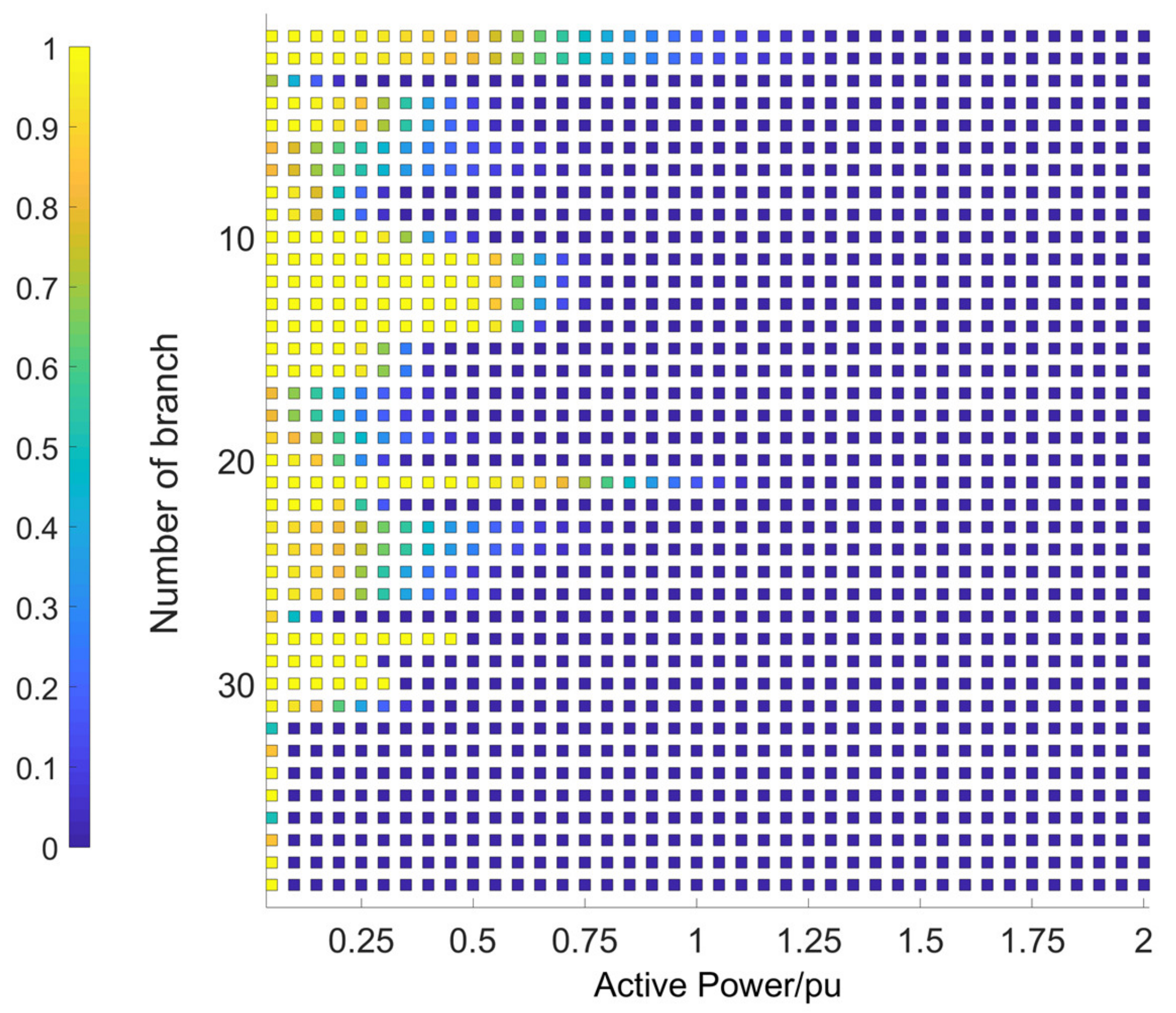
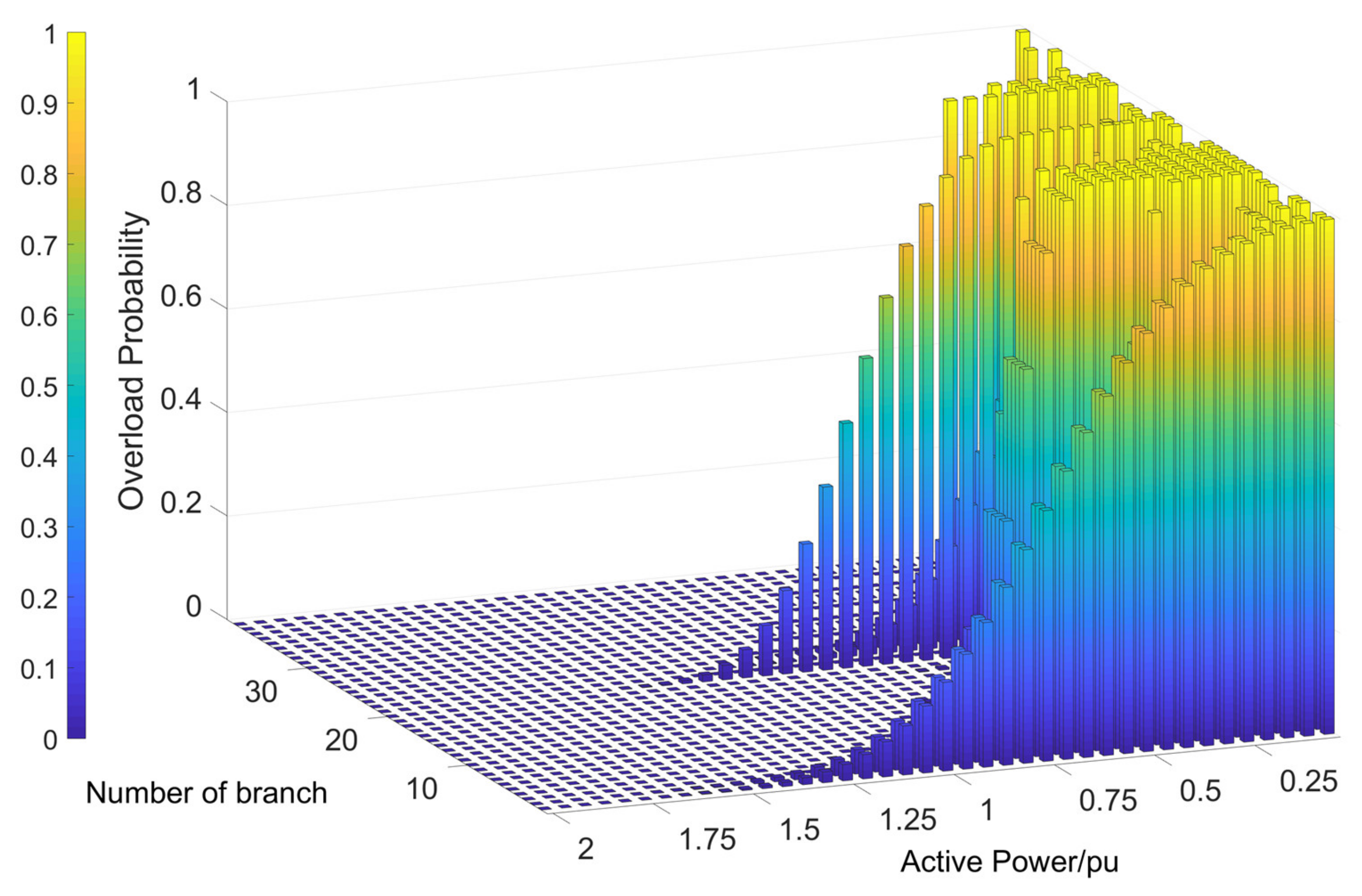
By analyzing Figure 9 and Figure 10, it can be seen that 1.2 pu was used as the over-limit standard. The limit-crossing probability of branch 1 and 2 were up to 4.69%. Therefore, in the comprehensive scenario, the overload probability of all branches was kept below 5%. The constraints of the optimization model were met, which demonstrates the effectiveness of the model in identifying potential problems and evaluating the system’s ability to maintain stability under different conditions. Validation of the performance of the proposed model highlights its value in the decision-making process related to load shedding strategies and risk mitigation measures.

7. Conclusions

This paper employed the South East Australian Power System as a case study to validate the effectiveness of the proposed method. It supplements the existing power system risk assessment framework by incorporating the analysis of extreme rainfall weather conditions. The main features of this method can be summarized as follows:
  • The proposed approach involves determining the rainfall curve and the corresponding water accumulation curve through the combined use of the SWMM model and the extreme learning machine. To assess the probabilities of different initial fault scenarios, the Monte Carlo sampling method was applied. Using statistical theory, the initial fault scenarios were refined, resulting in the identification of typical scenario sets. These sets comprised specific fault scenarios with their corresponding probabilities.
  • The branch power flow overload probability of each initial scenario within a single typical scenario set was calculated using the semi-invariant and Gram–Charlier series expansion methods. By applying the full probability formula, the power grid overload probability was obtained for each typical scenario set. This calculation took into account the probabilities of branch power flow overloads in the specific scenarios within the set. With the power grid overload probabilities determined for each typical scenario set, it was possible to calculate the power grid overload probability in the comprehensive scenario. This calculation involved aggregating the probabilities from all the typical scenario sets to provide an overall assessment of the likelihood of power grid transgressions.
  • In the optimal load curtailment model, the branch active power violation probability was incorporated as a constraint. This ensured that the power flow in each branch remained within the specified limits. To solve the constrained optimization problem, the particle swarm optimization (PSO) algorithm was employed. To handle the constraints, a penalty function approach was adopted, transforming the constrained optimization problem into an unconstrained one. This technique helped to speed up the solution process by converting the problem into a form that was more amenable to optimization algorithms such as PSO.

Author Contributions

Methodology, G.Z. and B.C.; Software, B.C.; Validation, J.S.; Investigation, G.Z.; Resources, Z.Q.; Writing–original draft, G.Z.; Writing–review & editing, L.W. All authors have read and agreed to the published version of the manuscript.

Funding

This research was funded by the Science and Technology Project of State Grid of Zhejiang Electric Power Company, Ltd. (Project Number: 2022-KJLH-BC-012).

Data Availability Statement

Data available in a publicly accessible repository. Refs. [24,33].

Conflicts of Interest

The authors declare that there are no conflict of interest.

References

  1. Yi, Z.; Chen, Z.; Yin, K.; Wang, L.; Wang, K. Sensing as the key to the safety and sustainability of new energy storage devices. Prot. Control. Mod. Power Syst. 2023, 8, 27. [Google Scholar] [CrossRef]
  2. Sun, X.; Zhang, Y.; Zhang, Y.; Wang, L.; Wang, K. Summary of Health-State estimation of lithium-ion batteries based on electrochemical impedance spectroscopy. Energies 2023, 16, 5682. [Google Scholar] [CrossRef]
  3. Wang, L.; Xie, L.; Yang, Y.; Zhang, Y.; Wang, K.; Cheng, S.J. Distributed online voltage control with fast PV power fluctuations and imperfect communication. IEEE Trans. Smart Grid 2023, 14, 3681–3695. [Google Scholar] [CrossRef]
  4. Ma, N.; Yin, H.; Wang, K. Prediction of the remaining useful life of supercapacitors at different temperatures based on improved long short-term memory. Energies 2023, 16, 5240. [Google Scholar] [CrossRef]
  5. Zhang, S.; Hosen, M.S.; Kalogiannis, T.; Mierlo, J.V.; Berecibar, M. State-of-health estimation of lithium-ion batteries based on electrochemical impedance spectroscopy: A review. Prot. Control. Mod. Power Syst. 2023, 8, 156. [Google Scholar]
  6. Zhang, H.; Gao, J.; Kang, L.; Zhang, Y.; Wang, L.; Wang, K. State of health estimation of lithium-ion batteries based on modified flower pollination algorithm-temporal convolutional network. Energy 2023, 283, 128742. [Google Scholar] [CrossRef]
  7. Zhou, G.; Shi, J.X.; Chen, B.J.; Qi, Z.Y.; Wang, L.C. Lightning protection measures and zoning lightning protection for transmission lines in medium and heavy ice areas. Electr. Porcelain Light. Arrester 2021, 4, 47–54. [Google Scholar]
  8. Zhou, G.; Shi, J.X.; Chen, B.J.; Qi, Z.Y.; Wang, L.C. Risk assessment of transmission line over-icing disaster considering multiple factors based on evolutionary strategy-projection tracing algorithm. Power Syst. Autom. 2013, 37, 92–97. [Google Scholar]
  9. Song, J.J. Time-Varying Outage Model for Overhead Transmission Lines under Severe Disasters; Zhejiang University: Hangzhou, China, 2013. [Google Scholar]
  10. Chen, Y. Research on Risk Assessment and Control of Wenzhou Power System Considering Extreme Weather; Zhejiang University: Hangzhou, China, 2022. [Google Scholar]
  11. Weinmann, R.; Cotilla-Sanchez, E.; Brekken, T.K. Toward Models of impact and recovery of the US Western Grid from earthquake events. Energies 2022, 15, 9275. [Google Scholar] [CrossRef]
  12. Swief, R.A.; Abdel-Salam, T.S.; El-Amary, N.H. Photovoltaic and wind turbine integration applying cuckoo search for probabilistic reliable optimal placement. Energies 2018, 11, 139. [Google Scholar] [CrossRef]
  13. Deng, X.; He, J.; Zhang, P. A novel probabilistic optimal power flow method to handle large fluctuations of stochastic variables. Energies 2017, 10, 1623. [Google Scholar] [CrossRef]
  14. Ye, X.; Wang, Y.F. Multipoint linearized probabilistic power flow calculation with correlation of random variables. J. Power Syst. Their Autom. 2023. [Google Scholar]
  15. Lian, H.R.; Zhou, B.R. Stochastic power flow resolution algorithm based on scenario partitioning. Power Grid Technol. 2017, 41, 3153–3160. [Google Scholar]
  16. Wei, P.; Liu, J.K. Stochastic power flow algorithm based on semi-invariant and Gram-Charlier level expansion method. Power Eng. Technol. 2017, 36, 34–38. [Google Scholar]
  17. Li, C.; Zeng, Y. An optimal dispatching method for power systems accounting for operational risks. J. Power Syst. Their Autom. 2016, 28, 73–79. [Google Scholar]
  18. Jia, Y.; Li, W.X. Penalty function improved particle swarm algorithm for optimal configuration of scenery storage system. J. Sol. Energy 2019, 40, 2071–2077. [Google Scholar]
  19. Bian, C.Y.; Fang, X.Y. Site selection model of electric power emergency material storage considering load level. J. Power Syst. Their Autom. 2017, 29, 78–83. [Google Scholar]
  20. Kang, W.Q. A security risk assessment method for power monitoring network based on improved AHP algorithm. Autom. Instrum. 2022, 10, 171–174. [Google Scholar]
  21. Wang, X.J.; Huang, Y. Comprehensive evaluation and type selection of energy storage based on hierarchical analysis method. Zhejiang Electr. Power 2022, 41, 1–8. [Google Scholar]
  22. Li, Q. SWMM-Based Reliability Analysis of Urban Stormwater Pipe Network and Multi-Objective Reconstruction Optimization Research; Dalian University of Technology: Dalian, China, 2016. [Google Scholar]
  23. Zhou, L.; Huang, Z.X. Extreme learning machine for short-term power system load forecasting. Electron. World 2021, 8, 33–34. [Google Scholar]
  24. Fu, L.H.; Liu, A.H. China Statistical Yearbook-2021; China Statistics Press: Beijing, China, 2022; pp. 68–70. [Google Scholar]
  25. Wang, S.S. Research on the Application of Production and Convergence Forecasting Models in Early Warning Systems; Nanchang University: Nanchang, China, 2019. [Google Scholar]
  26. Rui, X.F. Discovery and development of the production flow model. Adv. Water Resour. Hydropower Sci. Technol. 2013, 1, 1–6+26. [Google Scholar]
  27. Zhao, D.Q.; Chen, J.N. Study on the influence of sub-catchment delineation on SWMM simulation results. Environ. Prot. 2008, 8, 56–59. [Google Scholar]
  28. Zeng, X.T. Study on the Optimization Model of Stormwater Pipe Network Based on NSGA-II Algorithm Research; Southwest Jiaotong University: Chengdu, China, 2021. [Google Scholar]
  29. Xu, L. Power System Voltage Collapse Risk Assessment; Chongqing University: Chongqing, China, 2009. [Google Scholar]
  30. Zhang, W.T.; Fan, L.X. Wind power penetration power limit calculation based on DC probabilistic currents. Jiangsu Electr. Eng. 2014, 33, 1–4. [Google Scholar]
  31. Fan, J.H.; Xu, N. Fault recovery strategy for power distribution systems with distributed scenic power. Jiangsu Electr. Eng. 2014, 33, 1–4+8. [Google Scholar]
  32. Yang, R.; Zhang, Y. Multi-objective reactive power optimization of distribution network with improved particle swarm optimization. J. Anhui Eng. Univ. 2022, 37, 42–50. [Google Scholar]
  33. Gibbard, M.; Vowles, D. IEEE PES task force on benchmark systems for stability controls simplified 14-generator model of the south east Australian power system. Univ. Adel. 2014, 5005, 128. [Google Scholar]
Figure 1. The generation process of power facility fault scenarios.
Energies 16 06660 g001
Figure 2. Sampling process.
Energies 16 06660 g002
Figure 3. Flow chart of stochastic power flow algorithm.
Energies 16 06660 g003
Figure 4. Diagram of South East Australian Power System topology.
Energies 16 06660 g004
Figure 5. Three-dimensional plot of time, rainfall intensity, and probability density.
Energies 16 06660 g005
Figure 6. Three-dimensional plot of time, water depth, and probability density.
Energies 16 06660 g006
Figure 7. Failure scenarios and their corresponding probability histograms.
Energies 16 06660 g007
Figure 8. Bus load curtailment in each scenario.
Energies 16 06660 g008
Figure 9. The overload probability of each branch in the comprehensive scenario (2D).
Energies 16 06660 g009
Figure 10. The overload probability of each branch in the comprehensive scenario (3D).
Energies 16 06660 g010
Table 1. Data required for outage mode.
HeadingValue in the ModelHeadingValue in the Model
Catchment area/m215,000Pipe Manning roughness0.01
Flood width/m140Pipe diameter/m0.3
Catchment slope/%0.2Pipe bottom slope0.2
Permeable area ratio/%20Maximum permeability/(m·min−1)1.2
Manning roughness of impervious area0.013Minimum permeability/(m·min−1)0.06
Manning roughness of permeable area0.1Permeability attenuation coefficient (min−1)0.1
Table 2. Normal operating power for each branch of the South East Australian Power System.
BranchMVABranchMVABranchMVABranchMVA
1–650006–1580011–1280016–17800
2–950007–880011–128009–101000
3–850007–880011–148009–101000
4–1550007–980012–178009–101000
5–68008–1180014–168009–101000
5–68008–1180014–1780013–141000
6–78008–1180015–1680013–141000
6–128009–1280015–1680013–141000
6–1280010–13120015–1780013–141000
6–1580010–13120015–17800
Table 3. Total load curtailment in each typical scenario.
ScenariosTotal Load Curtailment (MVA)
Scenarios One132.49
Scenarios Two212.72
Scenarios Three345.22
Comprehensive scenarios162.63
Disclaimer/Publisher’s Note: The statements, opinions and data contained in all publications are solely those of the individual author(s) and contributor(s) and not of MDPI and/or the editor(s). MDPI and/or the editor(s) disclaim responsibility for any injury to people or property resulting from any ideas, methods, instructions or products referred to in the content.