Abstract
The application of electrical drives in the control of centrifugal fans and pumps is a well-established area that leads to substantial energy savings. It requires electrical and automation engineers to have some knowledge relevant to drives about fan and pump modelling since ignoring or oversimplifying fan/pump modelling for the intended drive design compromises the required control quality. This paper improves the existing dynamical models of fans and pumps integrated with induction motors via neural network estimation of overall fan/pump efficiency; this estimation is based on the voltage frequency of the driving induction motor, pressure, and flow rate, followed by the separation of the fan’s or pump’s own efficiency for the motor load torque computation, enhancing the accuracy due to the correct reflection of the power balance. The model is developed with a view to being convenient for control design applications. For the first time for dynamical models, it is verified experimentally, justifying the necessity of the first-order nonlinear differential equation for the flow rate. The validation includes a direct approach based on analysis of transient behaviour caused by a small-step perturbation of the frequency of the motor voltages and an indirect approach based on the introduced concept of the dynamical flow rate and pressure estimators.
1. Introduction and Literature Review
The application and control of induction motor drives for centrifugal fans and pumps in air and water supply systems is a well-established area, mainly driven by huge opportunities for energy saving. Air and water transportation in industrialised countries consumes more than 60% of total electrical energy converted into mechanical energy by induction motor drives [1]. Replacing the throttle/valve control of fans and pumps by variable frequency induction motor drive regulation provides savings of up to 30% of electrical energy, with a relatively short payback time for modernisation [2,3].
1.1. Ignoring and Oversimplifying Fan/Pump Modelling for Electrical Drives Design
In this area, research and design unavoidably require electrical and automation engineers to have some knowledge of centrifugal fans and pumps related to electrical drives and control, which should not be ignored or oversimplified [4]. An interesting and innovative adaptive scalar control is developed for the induction motor in [5], increasing the starting torque to its rated value. The intended application is for centrifugal fans, pumps, and belt conveyors. However, their influence on motor dynamics through the load torque is not accounted for in the control design procedure, which deteriorates the control performance.
The simplest way researchers can model the influence of fans and pumps on electrical motors is by setting their load torque as a parabolic static function of their velocity. This approach is used in [1], where an optimal vector control technique is designed based on Pontriagin’s maximum principle for a squirrel-cage induction motor driving a centrifugal pump. It minimises the motor’s copper loss in steady states and provides the shortest transient time between different operating points. It does not consider an optimisation of the overall pump’s efficiency, which is the product of the pump’s own efficiency and the electric drive’s efficiency. Similar oversimplified pump modelling was applied in the design of a solar-powered pump driven by a permanent magnet synchronous motor drive under vector control [6] and emulated via a DC generator torque control, which influences the accuracy of the simulations and tests. Paper [7] analyses the experimental performance of the solar-powered pump that is spun by a permanent-magnet DC motor, and it considers that the coefficients of the load torque parabolic function are constant, although they are subject to the characteristics of the hydraulic network connected to the pump (the system curves).
1.2. Quasi-Steady Fan/Pump Modelling for Electrical Drives Applications
Electrical and automation engineers dealing with the automation of air and water supply systems are well aware of the quasi-steady modelling of centrifugal fans and pumps, where the flow rate and pressure (head) change synchronously with the motor velocity change. These are steady-state dependences of the pressure (head) on the flow rate, the fan’s/pump’s shaft power on the flow rate, or the fan’s/pump’s efficiency on the flow rate for various constant velocities that were obtained experimentally [8] (also available in the fan/pump data sheets), represented as plots (Q–H, Q–P and Q–η curves, respectively) or analytical approximations, with a limited number of parameters to be determined from the plots. The affinity laws are applicable when the data are available only for the rated velocity [9]. This modelling proves that the power consumed for the transportation is proportional to the cubic velocity, justifying using variable speed drives for the fan/pump control; furthermore, its analysis leads to the standard recommendation of all industrial AC drive manufacturers to use V/f2 = constant scalar control for induction machine drives [10,11].
The required fan/pump motor’s rated power is computed based on quasi-steady modelling. Accurate motor sizing is important since oversizing increases the initial contractual cost for electrical services and the motor’s electrical losses [2], whereas undersizing leads to excessive demand penalties [2]. The effect of induction motor supply voltage (both sinusoidal and PWM) variation and unbalance on the motor and pump overall performance is explored experimentally and analysed using quasi-steady pump modelling [12,13].
Simulink/Simscape from Matlab offers three blocks for the quasi-steady modelling of centrifugal pumps in thermal and isothermal liquid networks and one block for a fan in a gas network. They are based on Q–H, Q–P, and Q–η curves or pump power loss approximations extended by affinity laws or look-up tables. They can be parameterised using data sheets or experimental fan/pump data and additionally contain geometrical parameters of the fans/pumps. They were used for the pump’s flow rate [14] and head [15] control modelling, but the variable speed drive models were relegated to gains. In [16], look-up-tables-based pump modelling that ignores drive dynamics is used for the simulation of a hybrid speed and throttle control.
The quasi-steady modelling is sufficient for justifying energy saving (fan/pump velocity control according to the demand) via steady-state analysis of possible operating points in Q–H and Q–P planes. However, in closed-loop systems like [14,15,16], it cannot be used for the analytical design of controllers. Controllers and their parameters are chosen intuitively.
1.3. Fan/Pump State Estimation Based on Electrical Drive Monitoring for Sensorless Control
In recent decades, experts in electrical drive control have established a new research direction by applying the principles of sensorless electric motor control to regulate fans and pumps. This approach aims to reduce the implementation costs of closed-loop energy-saving control for fans and pumps by eliminating the need for relatively expensive flow rates and pressure sensors. The quasi-steady modelling of fans and pumps has found wide application in the design of the required estimators based on the measurements already available in industrial drive monitoring systems.
The standard approach to estimate the flow rate and pressure (head) is developed using Q–H and Q–P curves for rated velocity (either experimental or datasheet) [17]. The principal disadvantage is that this estimate is reached via auxiliary estimates. The curves are modified using the affinity laws based on the motor angular velocity estimate, and the estimated motor shaft power is used to compute the flow rate and pressure (head) from the updated curves. Sometimes, the curves can contain flat parts, and the affinity laws become less accurate if the velocity changes more than 20% [18]. The system curve-based estimation [17] utilises the fan/pump load curve, the affinity laws, and the estimate of angular velocity. It is applicable when the parameters of the system curve are constant and known during the estimation.
Since the estimators are based on quasi-steady modelling, they are only assessed for steady-state operation. They can fail during transients. Otherwise, the control should be slow enough to consider it as quasi-steady.
1.4. Idea of Dynamical Fan/Pump Modelling for Electrical Drive Applications
The dynamical centrifugal fan/pump model was intuitively introduced in [19,20], where a first-order differential equation was added to a variation of a quasi-steady model. It describes the flow rate transients in the housing, and other algebraic approximation equations of the model are rearranged in a view convenient for control design. The model and all its later variations (the necessity of the differential equation for the flow rate and that no differential equation for the pressure is required) were never validated experimentally. It remains an assumption that restricts the model recognition by practical engineers (only quasi-steady models are available in Matlab/Simulink/Simscape). In both papers, the pressure (head) and the motor load torque developed by the pump are approximated by second-order polynomials (with different terms) in velocity and flow rate, and the pump efficiency is considered constant, which is feasible for a narrow control range. Extending the model in [19] with fault models and the two-phase induction machine model allows the fault detection algorithm to be designed analytically, using analytical redundancy relation and measuring only electrical variables of the motor and the head. An extended Kalman filtering is used in [20] to estimate the induction motor’s velocity and load torque with the following estimation of the flow rate and head via solving a third-order polynomial for the flow rate with coefficients depending on the velocity and load torque (quasi-steady design). Good matching between the estimated and real values is achieved in steady states, but the transients are made slower to reduce the dynamical error. Further improvement of the pump model is suggested in [21], where the overall (pump and motor) efficiency estimator is embedded into the model based on the computed flow rate and head. Instead of the efficiency estimator, the model in [22] is based on the drive’s consumed power estimation, and the load torque is determined using the difference between this estimation and the motor loss (only the copper loss is modelled).
1.5. Contributions of the Paper
The goal of the present paper is to fill the knowledge gap and make the dynamical centrifugal fan/pump model admitted by practical engineers and researchers for the purpose of analytical control and state estimation designs. Contrary to the reviewed papers above, which demonstrate applications of different models, this paper is focused on the features of the centrifugal fan/pump modelling and its integration with the induction motor model. The theory is developed for a centrifugal fan, but it is applicable for centrifugal pumps as well, with some minor changes since the principle of operation is the same.
The paper’s contributions to the dynamical modelling and state estimation are as follows:
- Compared to [19,20,21,22], a new approximation is used for the Q–H curve at rated velocity, allowing fans/pumps with a maximum point present in the curve to be modelled;
- Compared to [21], the induction motor load torque is computed based on the fan’s own efficiency, which is separated from the overall fan’s efficiency. This correctly reflects the power balance during the computation, improving the accuracy. The neural network estimator of the overall fan’s efficiency includes the frequency of the stator voltages of the induction motor as an additional input;
- The block diagram of the model is developed with a view to be convenient for electric drive control design and applications;
- For the first time for dynamical fan/pump models, this paper proves experimentally the necessity of the differential equation for the flow rate and shows that no differential equation is required for pressure. The validation is performed directly through the observation of the system behaviour due to small step perturbation in the frequency of the stator voltage;
- Indirect experimental validation of the model is provided via the design of neural network flow rate and pressure estimators based on experimental data. Using the authors’ results previously presented at the conference detailed in [23], it shows that the estimators designed based on quasi-steady modelling fail during transients, whereas the introduced dynamical estimators (with one neural network sample time delayed negative feedback, which is equivalent to accounting for the flow rate differential equation) succeed during both steady state and transient operation.
Section 2 presents analytical results on the dynamical fan’s modelling. Section 3 describes the test rig, the overall efficiency, the flow rate, and the pressure estimators’ design. Section 4 compares the model simulations against the experimental data and evaluates the quasi-steady and dynamical flow rate and pressure estimators.
2. Enhanced Dynamic Model of the Centrifugal Fan with Induction Motor Drive
The differential equation approximating the dynamics of the flow rate in the fan’s housing is shown below
where denotes the flow rate, is time, is the motor/fan angular velocity (a gearless drive is assumed), is the rated value of , is the pressure of the fan at zero flow rate and rated velocity, and are the approximation coefficients for the Q–H characteristic at , is the approximation coefficient of the duct air resistance characteristic and is an integration constant. The first term of the right side is the pressure at zero flow rate and arbitrary velocity updated based on the affinity law. Compared to the model in [20], the term is added, allowing for the modelling of a fan with a Q–H curve possessing a maximum point. For a pump model, a static head is added to the right side of (1).
The three first terms of the right side of (1) constitute the fan’s (pump’s) pressure
Similar to electrical circuits, the first terms on the right sides of (1) and (2) act as an idealised DC voltage source. The second and third terms are the internal drop of the voltage in the source, but it is a nonlinear function of the current . The last term in (1) is the voltage at the terminals of a nonlinear resistive load. Equation (1) is similar to the second Kirchhoff’s law, where the left side is an EMF induced across an inductor.
With , the solution of (1) gives the fan’s steady-state operating point (the intersection of the Q–H curves of the fan and the duct system). According to (1), the flow rate transients are longer than the transients of the velocity. However, according to (2), initially, the pressure changes synchronously with the velocity change, and later, the pressure transients are influenced by the flow rate dynamics. All parameters, except , can be determined either from datasheets or steady-state experimental data. The value of might vary for different operating points, and it can be determined experimentally only from dynamical tests.
Instead of the polynomial approximation in [19,20], the output power of the fan/pump (of the output stream) is computed directly as
The combined efficiency of the fan (pump) and its motor is computed as a ratio of the output power and the active input power of the motor ,
where is the motor’s efficiency and is the fan’s (pump’s) efficiency.
In [21] is embedded into the pump’s model as a neural network estimator with and as inputs. Further, is used to compute the load torque developed by the pump. This introduces inaccuracy into modelling because the motor loss is not eliminated from the computation. In the proposed modelling, , , and experimental data were used to compute the value for neural networks training. However, the neural network efficiency estimator is based on three inputs: (the frequency of the voltage supplied to the motor), and . Adding into the estimation algorithm enhances the accuracy since it is extracted directly from the control algorithm, whereas and are simulated values with a ±5% acceptable error.
The efficiency of the fan (pump) itself is
The efficiency of the motor is computed using the shaft power of the motor and the motor power loss .
where denotes the torque developed by the motor.
The induction motor loss mainly consists of copper loss, iron (magnetic) loss, and mechanical loss. The induction machine blocks available in Matlab/Simulink/Simscape account only for the copper loss and the mechanical loss can be easily introduced. Certainly, for higher accuracy, the modelling of induction machines accounting for iron loss can be used. Since the accuracy of the flow rate and pressure is not highly critical, and the parameterisation of the iron and mechanical loss is quite challenging, these losses can be attributed to the losses in the fan/pump. This assumption is to be verified further, and it will justify the convenient and quick use of the Simscape blocks for the fans/pumps control simulation.
The load torque developed by the fan (pump) at the motor shaft is determined as
Then,
The block diagram of the fan (pump, excluding the static head) based on Equations (1)–(9) is depicted in Figure 1.
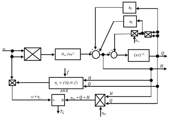
Figure 1.
The block diagram of the centrifugal fan.
The control input is , the outputs are , , and , and the disturbances are the changes in , , and . It is seen that the change of the velocity immediately causes a change in the pressure and, with some delay, in the flow rate. It leads to the load torque change, causing the velocity transients. This means that the transient time for all these variables is the same. The difference can be clearly shown during experimental testing of the transients caused by a small step change in frequency. Then, the system will behave closely to a linearised model. The initial velocity and pressure changes will happen with approximately the same time constant, and the initial flow rate transients will be slower.
The model is developed in a view usually used in the electrical drive control design. It is easy for parameterisation and integration with models of any type of AC electrical motor. It can be easily linearised for further analytical closed-loop control design. In this paper, it is combined with the standard two-phase model of a squirrel-cage induction motor based on five differential equations [20]. The stationary α-β stator reference frame is used because of the scalar velocity open-loop control implementation. The model is extended by the following equations:
where , and , denote the stator and rotor currents, respectively, and are the stator voltages, is the stator resistance, and is the rotor resistance. The loss in (10) includes only the copper loss . The mechanical and iron losses are attributed to the fan losses.
The Simulink/Simscape three-phase induction machine model block can be set to the stator stationary reference frame, and it provides access to both the stator and rotor currents. It is used further for simulations. The three-phase symmetrical stator phase voltages are generated by controlled voltage sources while maintaining the = const ratio, where denotes the amplitude of the stator voltages. The frequency is increased to the reference value via a ramp block.
3. Test Rig and Estimators Design
3.1. Test Rig Description
The test bench is implemented using the REM 48-0200-2D-07 industrial centrifugal fan manufactured by Nicotra-Gebhardt and shown in Figure 2. The datasheet’s best efficiency operating point is detailed in Table 1. The fan is driven by the 0.37 kW delta-connected Siemens three-phase squirrel-cage induction motor 1LA9070-2KA11-Z. The rated line-to-line voltage is 230 V, and the rated angular velocity is 2840 rpm. The parameters of the induction motor were determined experimentally via the standard no-load and locked rotor tests, using an identical motor in order not to disassemble the fan (the fan constantly develops the motor load torque, so the no-load test is impossible without dismounting the fan). They are presented in Table 2.
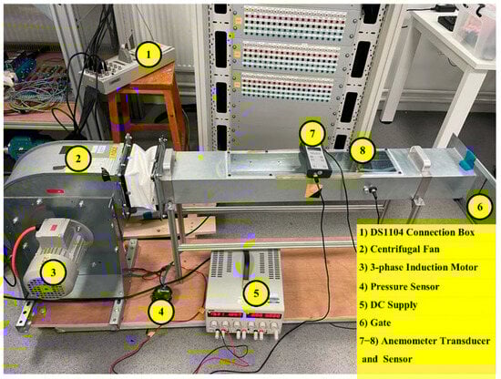
Figure 2.
The test bench of the fan.

Table 1.
The recommended operating point of the fan.
Table 2.
Induction motor parameters.
The induction motor is fed from a standard 3-phase full-bridge voltage source inverter (VSI) from the IRS26310DJ evaluation board. The VSI’s rated continuous output power is 400 W. The onboard PWM modulation is switched off. Instead, the sinusoidal PWM modulation is obtained from the PWM generator of the dSpace DS1104 controller board. This controller also provides the linear increase of the referred motor voltage frequency, the scalar V/f2 = constant regulation, and conversion of the output voltages of the DC link voltage sensor and the stator currents sensors into digital view. Digital isolators are used for galvanic isolation between the inverter and controller. This standard scalar velocity open-loop implementation is convenient for step response testing since there is no need to separate the fan transients from a complicated control system dynamic. More sophisticated techniques would require challenging separation of the fan/motor dynamics from the control system dynamics.
The test bench is equipped with the calibrated Anemometer HHF141 Omega (its turbine is mounted inside the air duct) and with the differential pressure sensor Ziehl Abegg DSG2000. The analogue outputs of both sensors are converted into digital views using the dSpace board. The experimental data are recorded through the dSpace ControlDesk 5.0 software.
3.2. Combined Efficiency Estimator Design
The gate is implemented at the output of the duct to manually regulate the air flow rate and pressure. The duct width is 11 cm.
Since the stator voltages are PWM signals, the reference instantaneous values of their fundamental components are used instead.
where , , and denote the voltages in phases a, b, and c, and superscript ‘*’ denotes the reference. The reference voltages and measured stator currents are converted into α and β components by applying Clarke transform for further and computation based on (11) and (12).
Steady-state testing is used for creating the training database to design the neural network estimator of the combined efficiency. The frequency of the stator voltages is kept constant at intervals of 2 Hz between 30 Hz and 50 Hz. For each constant frequency, the gate’s position varies between 0 and 11 cm of the duct width with a step of 1 cm. The gate’s positions of 0 and 11 cm mean the entirely open and entirely closed duct, respectively. For each operating point, the following data are collected: (reference value), and (measured values), and (computed value based on , , and ). In total, 132 operating points were recorded, as shown in Figure 3, including and the stator current amplitude. Note that this figure depicts eleven − and − characteristics of the fan for specific frequencies.
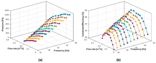
Figure 3.
Experimental characteristics of (a) and (b) .
The feed-forward backpropagation artificial neural network (ANN) architecture is used to implement the combined efficiency estimator—a 3-layer ANN is used with 5, 5, and 1 neurons in each layer. Activation functions are chosen as hyperbolic tansig for the first- and second-layer neurons and as purelin for the output layer. The ANN was created using Matlab’s ‘nntool’.
Several iterations were used to determine the first- and second-layer’s neuron minimum numbers to achieve the estimation accuracy illustrated in Figure 4 for the 132 operating points from Figure 3. Bayesian Regularization (trainbr) was utilised for the training procedure. The trained ANN is transformed into the Simulink model block by the ‘gensim’ Matlab command, and then, it is integrated into the Simulink model of the fan to compute the load torque.

Figure 4.
Discrepancy percentage between the ANN estimated efficiency and measured efficiency.
3.3. Flow Rate and Pressure ANN Estimators Design
The purpose of this section is to show how knowledge of centrifugal fan/pump modelling influences the design and quality of the ANN flow rate and pressure estimators. The best quality is considered as an indirect validation of the model. The following types of estimators are defined depending on the training data related to the fan modelling:
- Quasi-steady ANN estimators (type 1) trained using the test data of 132 steady-state operating points in Figure 3;
- Quasi-steady ANN estimators (type 2) trained based on dynamical experimental data;
- Dynamical ANN estimators trained using dynamical experimental data.
All types of pressure and flow rate estimators above are built based on ANNs with the feed-forward backpropagation architecture and include three layers. In all neurons, the hyperbolic tansig is utilised as an activation function, except the purelin was selected for the output layer neuron. All ANNs were created using the Matlab ‘nntool’ and trained using Bayesian Regularization (trainbr command in Matlab). Since the simulation and dSpace estimation implementation is based on Simulink, the ‘gensim’ command was applied to the trained ANNs to obtain the required Simulink blocks of the estimators.
The inputs of the quasi-steady estimators are the reference motor frequency, the measured stator current amplitude (based on instantaneous current values in three phases), and the estimated input active power of the motor. Compared to existing approaches utilising the estimated velocity and shaft power, the suggested technique includes only one input estimation. For the flow rate estimator of the first type, there are 3, 3, and 1 neurons (5, 5, and 1 for the second type) in the corresponding layers, whereas, for the pressure estimators, there are 5, 5, and 1 neurons [23]. The optimal neuron number was determined via a set of designs and simulations to meet the ISO 13348 standard accuracy. The term quasi-steady estimators was introduced to relate them to quasi-steady fan modelling (ANN without its own dynamics).
The introduced dynamical ANN estimators have the same inputs as the quasi-steady ones, and they have one additional input with the flow rate/pressure estimated at the previous ANN sample time to account for the first-order dynamics of the fan itself (ANN possessing its own dynamics). Except for this additional input, their architecture is identical to the second type of the quasi-steady estimators and is depicted in Figure 5, where z−1 denotes one sample time delay of the ANN. They are trained based on the same dynamic experimental data.
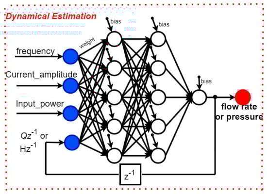
Figure 5.
Dynamical ANN estimation architecture.
4. Validation of the Fan Model
4.1. Direct Validation
The fan model is implemented in Matlab/Simulink/Simscape based on the diagram in Figure 1, and it is integrated with the model of the three-phase squirrel-cage induction motor, as explained in Section 2. The following parameters of the fan model were determined experimentally: = 1079 Pa, = 2039 Pa/(m3/s), = −1711 Pa/(m3/s)2, = 0.17 kg∙m2, and = 0.1 Pa∙s/(m3/s). The parameters of the motor are given in Section 3.1.
Initially, the start of the centrifugal fan from zero state is explored. The reference of the frequency of the stator voltages is increased linearly as a function of time till the rated value of 50 Hz is reached. Figure 6 and Figure 7 show the simulated and experimental transients of the fan’s pressure and flow rate when the position of the duct’s gate is 7 cm, which corresponds to = 10,936 Pa/(m3/s)2 during the simulations. The final operating point is close to the optimal data sheet point.
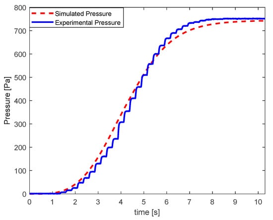
Figure 6.
Transients of the fan’s pressure during the start at 7 cm gate position.
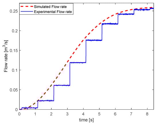
Figure 7.
Transients of the fan’s flow rate during the start at 7 cm gate position.
During the tests, it was found that the differential pressure sensor Ziehl Abegg DSG2000 had a sampling time of 0.2 s and included filtering, which can be observed in Figure 6. The anemometer HHF141 Omega had a sampling time of 1 s, which can be seen in Figure 7 (the operation is similar to a zero-order hold). The fan transients are slow enough to use these sensors and conclude the good matching between the simulations and experiments. Similar results were obtained where the position of the gate was 6 cm. Although the accuracy remains within the requirements, the step response tests are carried out further to prove the necessity of the differential Equation (1) in the fan modelling.
Figure 8 shows the experimental transients of the flow rate, pressure, and fan’s/motor’s velocity as deviations from their steady-state values at 50 Hz and 7 cm gate position. The transients are caused by a 2 Hz step decrease of the frequency. Due to the small value of the change, the initial step response behaviour is similar to step responses of aperiodic transfer functions. It can be seen that the flow rate time constant is bigger than the velocity time constant and that the pressure time constant is close (just slightly more) to . This observation justifies the use of differential Equation (1) in the centrifugal fan modelling and confirms that the pressure changes almost synchronously with the change of the shaft velocity (no extra differential equation is required). A2108 Optical Tachoprobe is used as a velocity sensor. To exclude the influence of the place of the flow rate sensor turbine installation within the duct, the following simple computations are done. The cross-section of the duct is 0.0146 m2. The air velocity in the duct is 0.258/0.0146 = 17.67 m/s. The distance of the turbine position from the fan output is 0.78 m. Then, the time for the air from the fan to reach the turbine is 0.0441 s, and this is significantly smaller than . Therefore, the contribution of the place of the turbine installation into can be neglected.
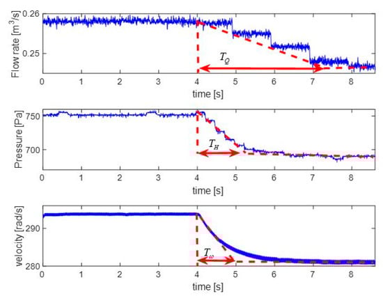
Figure 8.
Experimental step response of the system from 50 Hz to 48 Hz at gate position 7.
Figure 9 demonstrates the results of the model simulation, with the increased integration constant = 5000 Pa∙s/(m3/s), to be close to the experimental data in Figure 8. This shows that the added first-order flow rate differential equation is sufficient for good matching with the experimental transients. The maximum simulation dynamical errors for the flow rate, pressure, and velocity are 1.2%, 2.2%, and 2.5%, respectively, compared to the corresponding experimental transients in Figure 8. If the value of decreases to 0.1 Pa∙s/(m3/s), the model becomes closer to the quasi-steady one. For this case, all three time constants were obtained close to each other (see Figure 10), which contradicts the experiments. Therefore, the determination of the for specific operating points (narrow control ranges) should be done based on the step responses and not based on the starting-from-zero test.
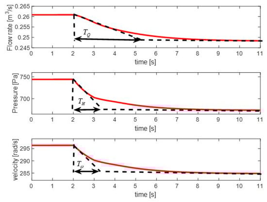
Figure 9.
Simulated step response of the system from 50 Hz to 48 Hz at gate position 7.
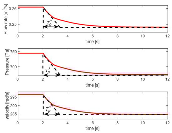
Figure 10.
Simulated step response of the system with smaller , from 50 Hz to 48 Hz at gate position 7.
Similar experimental and simulation results were obtained for 1 Hz and 2 Hz frequency step changes from different initial frequencies and at different gate positions, which validates the model and justifies the initial assumptions.
4.2. Indirect Validation—Flow Rate and Pressure Estimations
Figure 11 shows the operation of the quasi-steady pressure and flow rate ANN estimators (type 1) during experimental transients caused by the frequency step changes and smooth change of the gate position from 7 cm to 6 cm. It can be observed that these estimators fail during transients (the dynamical error can be more than 100%). A sensorless closed-loop control system based on them must be implemented quite slow to be considered quasi-steady.

Figure 11.
Simulated quasi-steady ANN estimations (type 1): conditions (a) pressure (b) and flow rate (c) © 2022 IEEE [23].
The experimental transients in Figure 11, including the recorded input active power and current amplitude, were used to train the quasi-steady estimators (type 2). Figure 12 illustrates the operation of these estimators during the experimental transients used for training. Despite the dynamical training data being used, there appear to be some spikes (maximum 4% and 6% dynamical errors for the pressure and flow rate, respectively), which will cause disturbances in the pressure/flow rate closed loops.
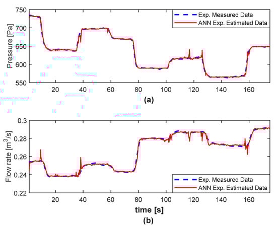
Figure 12.
Pressure (a) and flow rate (b) quasi-steady estimation (type 2) © 2022 IEEE [23].
The dynamical ANN estimators are trained based on the experimental transients in Figure 11 as well. Figure 13 shows their estimation during the recorded experimental transients used for training. The quality of the dynamical estimation is better than for the quasi-steady estimators. The estimation for experimental transients not used in training is also in good agreement with the test data [23]. This means that the introduced first-order estimators’ dynamics correctly reflect the dynamical centrifugal fan/pump modelling.
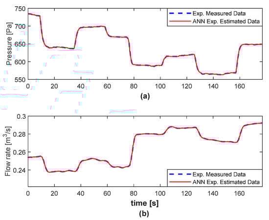
Figure 13.
Pressure (a) and flow rate (b) dynamical estimation © 2022 IEEE [23].
5. Conclusions
This paper improves the existing dynamical models of the centrifugal fan/pump with induction motor drive via neural network estimation of the fan’s/pump’s overall efficiency. The method is based on the voltage frequency of the driving motor, pressure, and flow rate as the estimators’ inputs, with the following separation of the fan’s/pump’s own efficiency for the motor load torque computation to enhance the accuracy due to the correct reflection of the power balance. The fan’s/pump’s model is developed with a view to being convenient for sensored and sensorless analytical control design applications. Electrical and automation engineers working with water and air supply system automation will find it simple to understand and parameterise. For the first time, the dynamical model is verified experimentally based on the step response, justifying the necessity of the first-order nonlinear differential equation for the flow rate. During the step response tests from a steady state close to the best efficiency operating point, the maximum simulation dynamical errors for the flow rate, pressure, and velocity were 1.2%, 2.2%, and 2.5%, respectively, compared to the corresponding experimental transients. This knowledge is applied to explain the failure of the quasi-steady pressure and flow rate estimators during transients. Accordingly, dynamical estimators are designed to fix this problem, which also provides the indirect validation of the model. Further exploration of the dynamical modelling can include verification for alternative types of driving motors, like synchronous reluctance motors [24] and line-start permanent-magnet synchronous motors [25], and searching for other application areas except for analytical control design, estimations, and fault detections.
Author Contributions
Conceptualisation, C.T. and O.K.; methodology, C.T. and O.K.; software, C.T.; validation, C.T. and O.K.; formal analysis, C.T. and O.K.; writing—original draft preparation, writing—review and editing, C.T. and O.K.; supervision, O.K.; funding acquisition, O.K. All authors have read and agreed to the published version of the manuscript.
Funding
This work, in part, was conducted within the research project ‘Joint UK-India Clean Energy Centre (JUICE)’, which is funded by the RCUK’s Energy Programme (contract no: EP/P003605/1). The project funder was not directly involved in the writing of this article.
Data Availability Statement
The data presented in this study are available on request from the corresponding author.
Conflicts of Interest
The authors declare no conflict of interest.
References
- Arribas, J.R.; González, C.M.V. Optimal Vector Control of Pumping and Ventilation Induction Motor Drives. IEEE Trans. Ind. Electron. 2002, 49, 889–895. [Google Scholar] [CrossRef]
- Corgnati, S.P.; Mitolo, M.; Orlietti, L.; Tartaglia, M. Energy Savings in Integrated Urban Water Systems: A Case Study. IEEE Trans. Ind. Appl. 2017, 53, 5150–5154. [Google Scholar] [CrossRef]
- Eto, J.H.; De Almeida, A. Saving Electricity in Commercial Buildings with Adjustable-Speed Drives. IEEE Trans. Ind. Appl. 1988, 24, 439–443. [Google Scholar] [CrossRef]
- Weigand, H.A.; Eddy, L.B. Centrifugal Pump and Compressor Characteristics. Electr. Eng. 1960, 79, 576–582. [Google Scholar] [CrossRef]
- Travieso-Torres, J.C.; Contreras-Jara, C.; Diaz, M.; Aguila-Camacho, N.; Duarte-Mermoud, M.A. New Adaptive Starting Scalar Control Scheme for Induction Motor Variable Speed Drives. IEEE Trans. Energy Convers. 2022, 37, 729–736. [Google Scholar] [CrossRef]
- Murshid, S.; Singh, B. Double Stage Solar PV Array Fed Water Pump Driven by Permanent Magnet Synchronous Motor. IEEE Trans. Ind. Appl. 2021, 57, 1736–1745. [Google Scholar] [CrossRef]
- Kolhe, M.; Joshi, J.C.; Kothari, D.P. Performance analysis of a directly coupled photovoltaic water-pumping system. IEEE Trans. Energy Convers. 2004, 19, 613–618. [Google Scholar] [CrossRef]
- Emami, S.A.; Emami, M.H. Design and Implementation of an Online Precise Monitoring and Performance Analysis System for Centrifugal Pumps. IEEE Trans. Ind. Electron. 2017, 65, 1636–1644. [Google Scholar] [CrossRef]
- Pottebaum, J.R. Optimal Characteristics of a Variable-Frequency Centrifugal Pump Motor Drive. IEEE Trans. Ind. Appl. 1984, IA-20, 23. [Google Scholar] [CrossRef]
- Altivar Machine ATV320 Variable Speed Drives for Asynchronous and Synchronous Motors Installation Manual. 2020, p. 149. Available online: https://download.schneider-electric.com (accessed on 17 November 2022).
- ACS550 User’s Manual ACS550-01 Drives (0.75…160 kW) ACS550-U1 Drives (1…200 hp). p. 145. Available online: https://library.e.abb.com (accessed on 17 November 2022).
- Kini, P.G.; Bansal, R.C. Effect of Voltage and Load Variations on Efficiencies of a Motor-Pump System. IEEE Trans. Energy Convers. 2010, 25, 287–292. [Google Scholar] [CrossRef]
- Kini, P.G.; Bansal, R.C.; Aithal, R.S. Performance Analysis of Centrifugal Pumps Subjected to Voltage Variation and Unbalance. IEEE Trans. Ind. Electron. 2008, 55, 562–569. [Google Scholar] [CrossRef]
- Gevorkov, L.; Rassolkin, A.; Kallaste, A.; Vaimann, T. Simulink Based Model for Flow Control of a Centrifugal Pumping System. In Proceedings of the 25th International Workshop on Electric Drives: Optimization in Control of Electric Drives, IWED 2018, Moscow, Russia, 31 January–2 February 2018; pp. 1–4. [Google Scholar] [CrossRef]
- Gevorkov, L.; Vodovozov, V.; Raud, Z. Simulation Study of the Pressure Control System for a Centrifugal Pump. In Proceedings of the 57th International Scientific Conference on Power and Electrical Engineering of Riga Technical University, RTUCON 2016, Riga, Latvia, 13–14 October 2016; pp. 1–5. [Google Scholar] [CrossRef]
- Gevorkov, L.; Smidl, V.; Sirovy, M. Model of Hybrid Speed and Throttle Control for Centrifugal Pump System Enhancement. In Proceedings of the IEEE International Symposium on Industrial Electronics, Vancouver, BC, Canada, 12–14 June 2019; pp. 563–568. [Google Scholar] [CrossRef]
- Ahonen, T.; Tamminen, J.; Ahola, J.; Kestilä, J. Frequency-Converter-Based Hybrid Estimation Method for the Centrifugal Pump Operational State. IEEE Trans. Ind. Electron. 2012, 59, 4803–4809. [Google Scholar] [CrossRef]
- Tamminen, J.; Viholainen, J.; Ahonen, T.; Ahola, J.; Hammo, S.; Vakkilainen, E. Comparison of Model-Based Flow Rate Estimation Methods in Frequency-Converter-Driven Pumps and Fans. Energy Effic. 2014, 7, 493–505. [Google Scholar] [CrossRef]
- Kallesøe, C.S.; Cocquempot, V.; Izadi-Zamanabadi, R. Model Based Fault Detection in a Centrifugal Pump Application. IEEE Trans. Control Syst. Technol. 2006, 14, 204–215. [Google Scholar] [CrossRef]
- Kiselychnyk, O.I.; Bodson, M. Nonsensor Control of Centrifugal Water Pump with Asynchronous Electric-Drive Motor Based on Extended Kalman Filter. Russ. Electr. Eng. 2011, 82, 69–75. [Google Scholar] [CrossRef]
- Burian, S.O.; Kiselychnyk, O.I.; Pushkar, M.V.; Reshetnik, V.S.; Zemlianukhina, H.Y. Energy-Efficient Control of Pump Units Based on Neural-Network Parameter Observer. Tech. Electrodyn. 2020, 2020, 71–77. [Google Scholar] [CrossRef]
- Pechenik, M.; Kiselychnyk, O.; Buryan, S.; Petukhova, D. Sensorless Control of Water Supply Pump Based on Neural Network Estimation. Electrotech. Comput. Syst. 2015, 3, 462–466. [Google Scholar]
- Turkeri, C.; Kiselychnyk, O. Dynamical Flow Rate and Pressure Artificial Neural Network Estimators for a Centrifugal Fan Driven by an Induction Motor Drive. In Proceedings of the IEEE 1st Industrial Electronics Society Annual On-Line Conference (ONCON), Kharagpur, India, 9–11 December 2022; pp. 1–6. [Google Scholar] [CrossRef]
- Gevorkov, L.; Domínguez-García, J.L.; Rassõlkin, A.; Vaimann, T. Comparative Simulation Study of Pump System Efficiency Driven by Induction and Synchronous Reluctance Motors. Energies 2022, 15, 4068. [Google Scholar] [CrossRef]
- Goman, V.; Oshurbekov, S.; Kazakbaev, V.; Prakht, V.; Dmitrievskii, V. Energy Efficiency Analysis of Fixed-Speed Pump Drives with Various Types of Motors. Appl. Sci. 2019, 9, 5295. [Google Scholar] [CrossRef]
Disclaimer/Publisher’s Note: The statements, opinions and data contained in all publications are solely those of the individual author(s) and contributor(s) and not of MDPI and/or the editor(s). MDPI and/or the editor(s) disclaim responsibility for any injury to people or property resulting from any ideas, methods, instructions or products referred to in the content. |
© 2023 by the authors. Licensee MDPI, Basel, Switzerland. This article is an open access article distributed under the terms and conditions of the Creative Commons Attribution (CC BY) license (https://creativecommons.org/licenses/by/4.0/).