Using Deep Neural Network Methods for Forecasting Energy Productivity Based on Comparison of Simulation and DNN Results for Central Poland—Swietokrzyskie Voivodeship

Abstract

Forecasting electricity demand is of utmost importance for ensuring the stability of the entire energy sector. However, predicting the future electricity demand and its value poses a formidable challenge due to the intricate nature of the processes influenced by renewable energy sources. Within this piece, we have meticulously explored the efficacy of fundamental deep learning models designed for electricity forecasting. Among the deep learning models, we have innovatively crafted recursive neural networks (RNNs) predominantly based on LSTM and combined architectures. The dataset employed was procured from a SolarEdge designer. The dataset encompasses daily records spanning the past year, encompassing an exhaustive collection of parameters extracted from solar farm (based on location in Central Europe (Poland Swietokrzyskie Voivodeship)). The experimental findings unequivocally demonstrated the exceptional superiority of the LSTM models over other counterparts concerning forecasting accuracy. Consequently, we compared multilayer DNN architectures with results provided by the simulator. The measurable results of both DNN models are multi-layer LSTM-only accuracy based on R2—0.885 and EncoderDecoderLSTM R2—0.812.

1. Introduction

Poland’s photovoltaic (PV) sector has been witnessing a consistent upswing, with various factors contributing to the advancement of photovoltaic technology in the nation. Similar to many other European Union (EU) member states, Poland has established ambitious renewable energy targets to bolster the proportion of renewables in its energy mix. Consequently, this impetus has triggered substantial investments in solar energy and PV technology. The government has proactively introduced diverse support mechanisms, such as feed-in tariffs, auctions, and subsidies, to foster the growth of renewable energy initiatives, including solar PV installations. Being an EU member state, Poland enjoys access to funding programs that facilitate the transition to renewable energy sources, which has further accelerated the development of photovoltaic projects in the country. Encouragingly, the cost of PV technology has been consistently declining over the years, rendering solar energy increasingly economically viable and appealing to both investors and consumers alike. Simultaneously, there has been a concerted effort to reduce dependence on imported fossil fuels, leading to a notable emphasis on fostering domestic renewable energy sources, including solar power. Notably, investments in PV technology have enabled Poland to diversify its energy sources, thereby significantly bolstering energy security [1]. A remarkable milestone occurred between 2019 and 2022, as over one million new PV micro-installations were established, primarily focusing on single-family households [2]. These PV micro-installations are thoughtfully tailored to align with specific energy consumption patterns, spanning distinct periods, such as a year, adhering dutifully to prosumer rules within Poland’s regulatory framework.

The principal aim of this study centers around evaluating the feasibility and precision of employing PV energy production calculation methods under Polish conditions. Researchers have observed that presently utilized methods for calculating energy production may exhibit inaccuracies stemming from inadequate adaptation to terrain, location, wind conditions, and the representative characteristics of PV panels within the installation. In this research, the application of deep neural network (DNN) methods will be explored to verify the accuracy of data provided by SolarEdge, a widely renowned simulator. Emphasis will be placed on hybrid long short-term memory (LSTM)-based architectures to carry out this assessment effectively.

Furthermore, the statistical analysis conducted in this study meticulously evaluates representative characteristics of the one-year analysis period. This comprehensive investigation marks the first-ever assessment of energy production from a micro-inverter installation under simulated conditions within Central Eastern Europe, specifically in the Swietokrzyskie Voivodeship region.

2. Materials and Methods

Simulation-based methods and AI predictions represent distinct approaches applied in the estimation of electricity generation from renewable energy sources (RES) [3]. Let us delve into each of these methodologies.

2.1. Simulation-Based Techniques

Simulation-based methods entail the development of computer models that emulate the behavior of renewable energy systems under various conditions. These models consider a myriad of factors, including weather patterns, geographical location, technical specifications of renewable energy sources (PV farms), and the unique characteristics of the energy grid.

Advantages of Simulation-Based Methods:

• Precision: Simulation models can offer precise predictions when properly calibrated and grounded in real-world data.
• Flexibility: They can be tailored to accommodate diverse scenarios and configurations.
• Understanding: Simulations facilitate comprehension of the intricate interactions between different components within the energy system.

Disadvantages of Simulation-Based Methods:

• Computational Intensity: Developing and executing simulations can be computationally demanding, particularly for large-scale systems.
• Data Requirements: High-quality data pertaining to weather, energy demand, and system parameters are crucial for ensuring accurate simulations.
• Complexity: Constructing a reliable simulation model necessitates expertise and domain knowledge.

2.2. AI Predictions for Electricity Generation

AI predictions encompass the use of machine learning algorithms, such as neural networks, to scrutinize historical data and make forecasts regarding future electricity generation from renewable sources. These algorithms discern patterns and relationships from data and can generate projections based on these identified patterns.

Advantages of AI Predictions:

• Speed: AI models can rapidly process vast datasets and provide real-time predictions.
• Adaptability: They possess the ability to adapt to changing conditions and learn from newly acquired data.
• Scalability: AI models demonstrate efficacy in handling large-scale systems.

Disadvantages of AI Predictions:

• Data Quality: The accuracy of AI predictions heavily relies on the quality and sensitive character of the training data.
• Black-Box Nature: Neural networks can be challenging to interpret, making it difficult to comprehend the underlying reasoning behind predictions.
• Limited Generalization: AI models may encounter difficulties when dealing with unseen situations or data that significantly deviate from the training set.

Combining Both Approaches: In practice, a hybrid approach, integrating simulation-based methods and AI predictions, emerges as a viable solution to capitalize on the strengths of each technique. For instance, simulation models can furnish synthetic training data for AI models, augmenting their accuracy. Moreover, AI models can optimize specific parameters within the simulation model, thereby enhancing overall performance [4].

Ultimately, the selection between simulation-based methods and AI predictions hinges on factors such as the availability of data, the complexity of the RES system, the desired level of accuracy, and the computational resources at hand. In numerous cases, a combined methodology presents the most robust and dependable outcomes [5].

2.3. ML Methods for Predictions of Electricity Generation

Below, we would like briefly describe methods that could also be used in particular analyzed scenarios.

2.3.1. Random Forest (RF)

In this innovative approach, we leverage the collective power of multiple average-quality models to outperform their individual capabilities. The underlying concept is to amalgamate the random errors inherent in individual models through averaging, resulting in remarkably accurate final predictions. A crucial requirement is that the models contributing to the average exhibit significant diversity. To realize this concept, we adopt a strategy akin to a random forest, where simple decision trees serve as the medium-quality constituents.

The pivotal hyperparameters for this technique involve the depth of each individual tree and the total count of trees within the ensemble. The introduction of diversity among trees hinges on two primary mechanisms. Firstly, each tree is trained on a distinct learning subset, generated through bootstrap sampling from the entire training set. Secondly, a subset of learning attributes is randomly chosen, ensuring that each tree is founded on different variables. Consequently, the repetition of the same features is mitigated. Notably, this methodology has proven its mettle in diverse machine-learning competitions, solidifying its effectiveness in the realm of machine-learning endeavors [6].

2.3.2. XGBoost

In contrast to the forest-style approach, XGBoost embraces the sequential construction of trees in a boosting framework. While both methods utilize random trees, XGBoost capitalizes on a sequential strategy. Each subsequent tree aims to optimize the prediction of residuals left unexplained by its predecessors. In essence, the new predictor is tailored to rectify the residual errors introduced by the previous predictor. This sequential refinement process continually enhances the overall predictive performance of the model.

The adoption of these methodologies is pervasive in practical applications. Our investigation harnesses the XGBoost library implementation, renowned for its exceptional speed and accuracy. Among the explored hyperparameters are the maximum number of leaves per tree, the count of gradient-reinforced trees, and a regularization-controlling parameter known as the learning rate. This comprehensive exploration contributes to fine-tuning the XGBoost model for optimal results.

2.4. Analyzed Designed PV Farm

Data for further research were downloaded from SolarEdge designer:

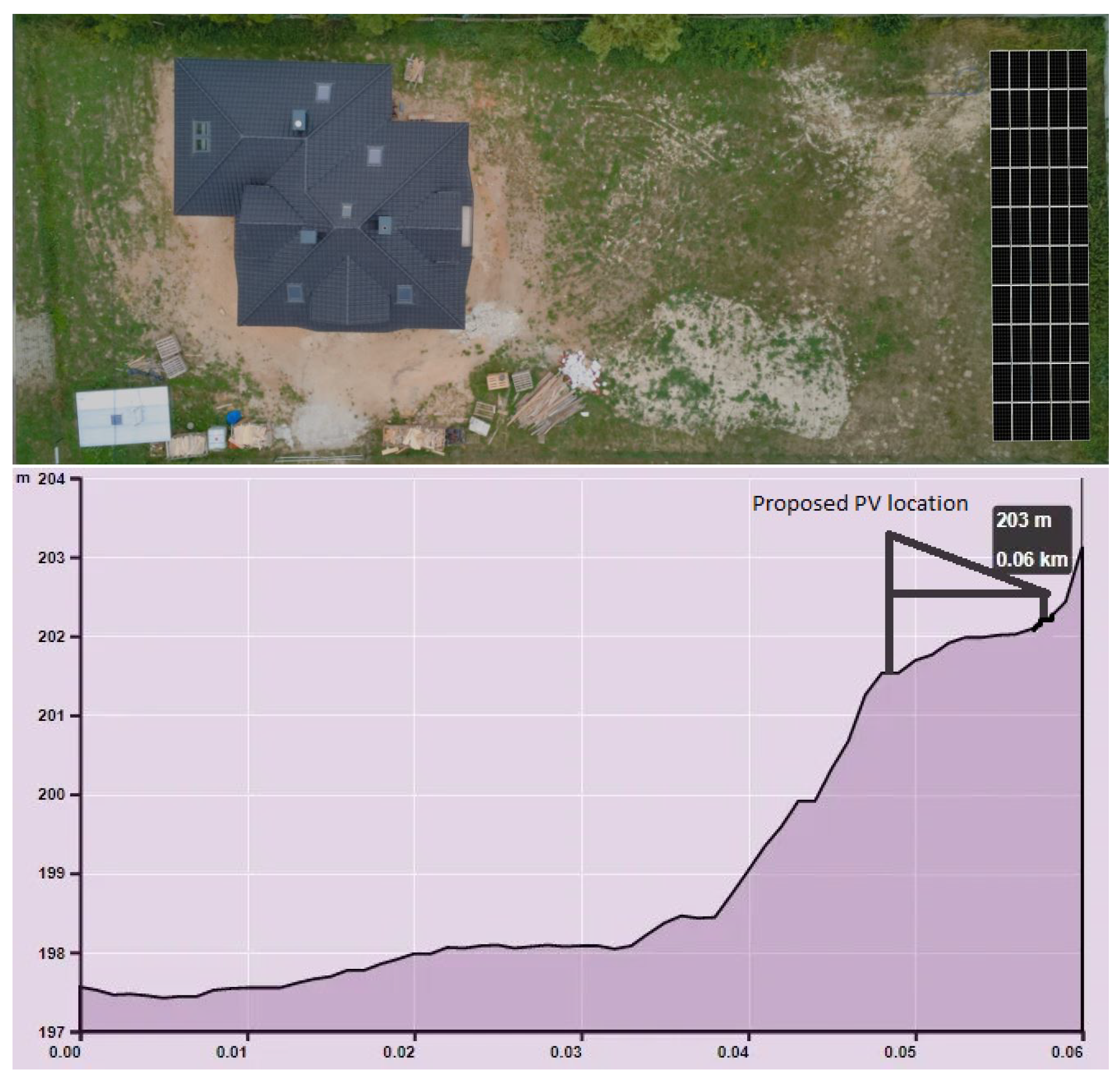
• The PV farm has a total installed DC power capacity of 27.25 kilowatts peak (KWp). This is achieved through the use of 50 JAM72D30-545/MB solar panels (Figure 1).
• The PV system utilizes a Solar Edge SE25K inverter, which has a capacity of 25,000 watts. The inverter converts the DC power generated by the solar panels into AC power, suitable for use in homes and businesses (Figure 2).
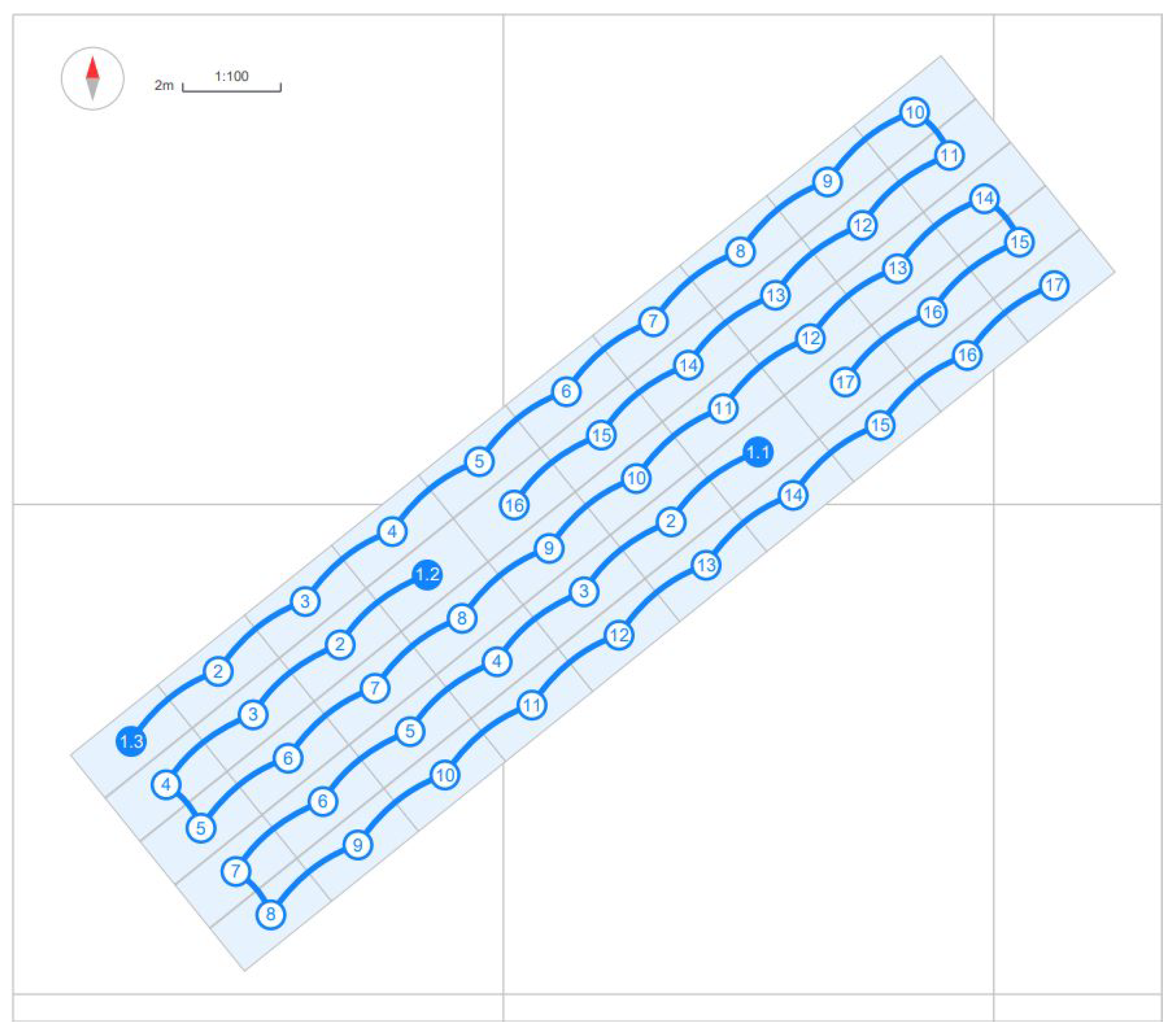
• To maximize energy production and improve efficiency, the PV farm is equipped with 50 Solar Edge S650B optimizers. These optimizers individually track and optimize the performance of each solar panel, ensuring that the entire system operates at its highest potential (Figure 3).
• The maximum AC power output of the PV farm is 25 kilowatts (KW). This represents the highest amount of electricity that the system can produce and supply to the grid or connected loads at any given moment.
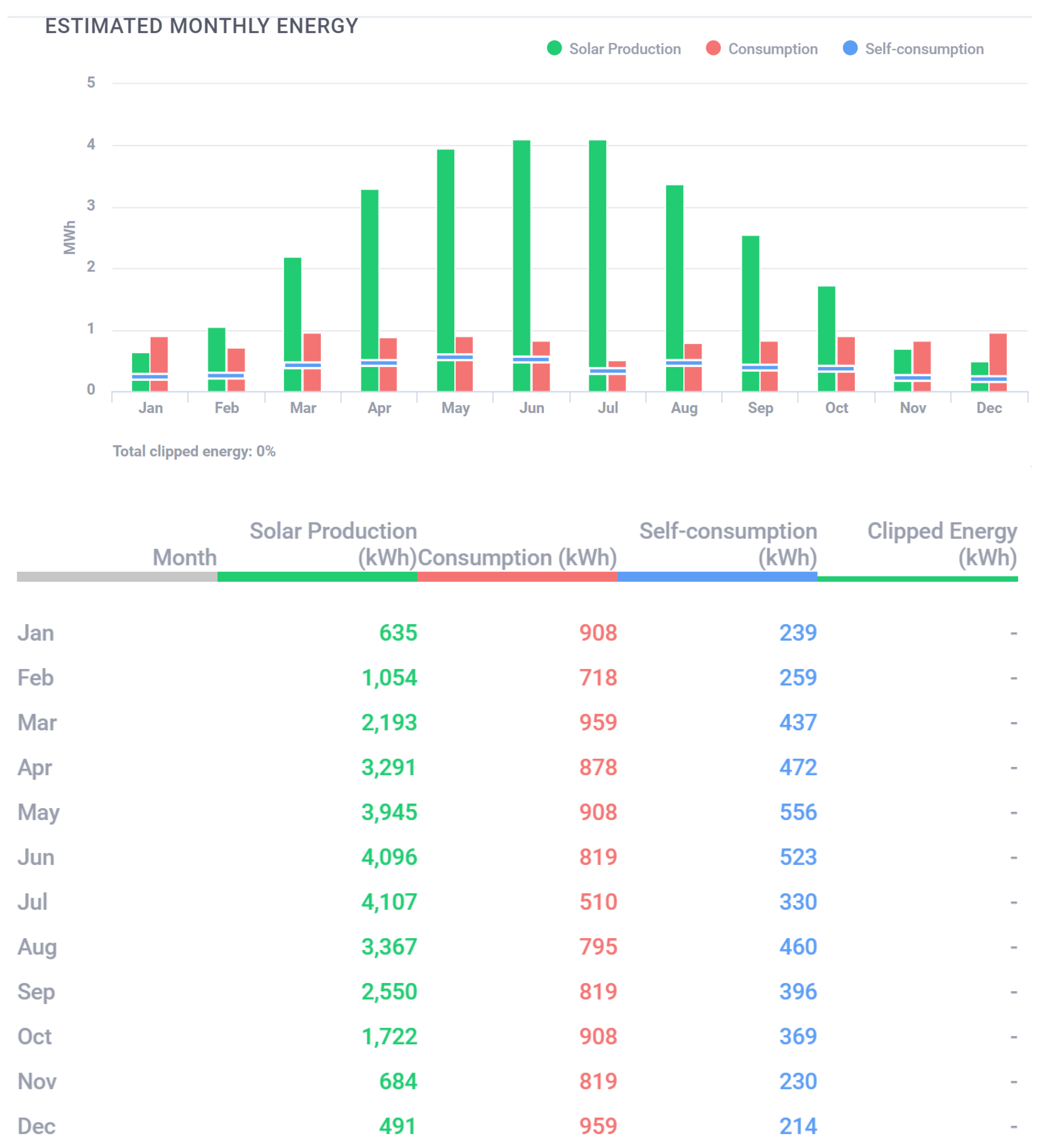
• The PV farm’s estimated annual energy production is 28.10 megawatt-hours (MWh). This figure indicates the total amount of electricity the system is expected to generate over the course of a year under average sunlight conditions (Figure 4).
• The performance index of the PV farm is 91%. This metric represents the efficiency of the system in converting sunlight into electricity. An index of 91 suggests that the PV farm is performing at a high level of efficiency, considering various factors such as shading, temperature, and soiling losses.

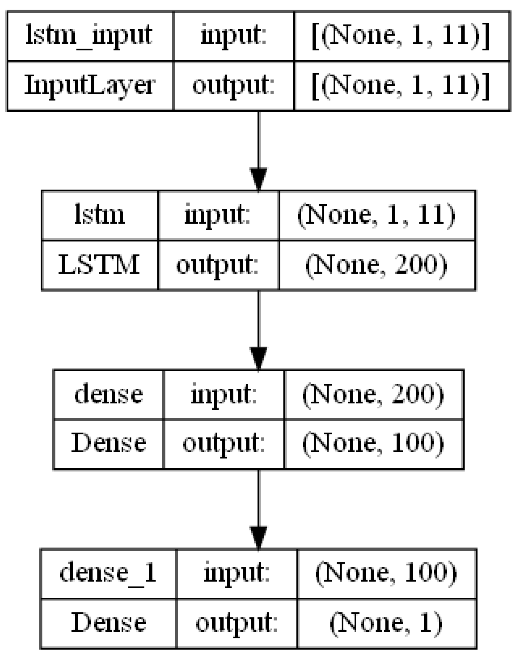
2.5. MultiLSTM DNN Model Architecture

A hybrid DNN-LSTM model combines the strengths of deep neural networks (DNNs) and long short-term memory (LSTM) [7] networks to tackle complex problems involving sequential data [8]. In the described model, we integrate the capabilities of DNNs for capturing high-level patterns from data with the sequence modeling capabilities of LSTMs [9]. This combination is particularly useful when you want to handle both the inherent sequential nature and intricate relationships in the data. Below architecture was presented (Figure 5).

The first layer is an LSTM (long short-term memory) layer: In this model, the LSTM layer has 200 units (also referred to as cells or neurons). The activation function used within each LSTM unit is a rectified linear unit (ReLU), which introduces non-linearity to the network. Following the LSTM layer is a dense fully connected layer. This layer contains 100 units and employs the ReLU activation function. The purpose of this layer is to learn higher-level features and patterns from the output of the LSTM layer. It adds a level of non-linearity and abstraction to the model’s representation. The final layer is the output layer. The activation function for this layer is not explicitly specified in the provided code, so it might default to a linear activation. This layer produces the final predictions of the model.

MultiLSTMDNN Hyperparameters

Hyperparameters used for the given architecture:

• LSTM units in the encoder and decoder layers: 200 units each.
• Activation function used in the LSTM and dense layers: ReLU (rectified linear unit).
• First dense unit (fully dense connected layer) with number of 100 units
• Output layer: 1 unit.
• Optimizer: Adam

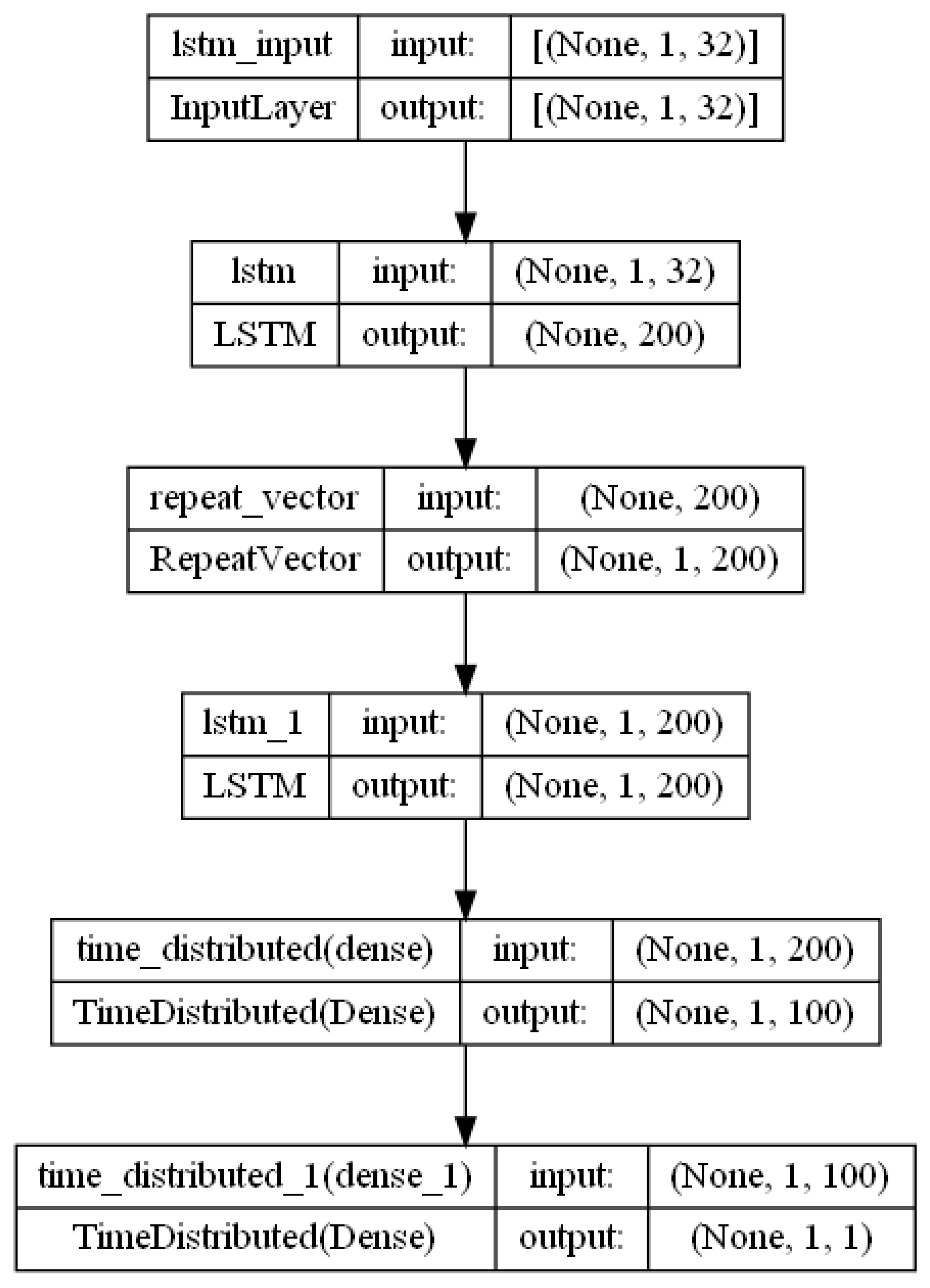
2.6. EncoderDecoder DNN Model Archiecture

The second architecture used in this project is EncoderDecoder LSTM-based architecture. The picture below visualizes it (Figure 6).

The foremost stratum manifests as an LSTM layer, outfitted with 200 units, effectively functioning as an encoder. Its fundamental role involves imbibing the inherent structure and information encapsulated within the input sequences. Through the utilization of the rectified linear unit (ReLU) activation function, the encoder imparts a layer of non-linearity to its transformations.

Subsequently, a RepeatVector layer follows, duplicating the encoded representation a requisite number of times to align with the intended span of output time steps This operation primes the encoded representation for subsequent ingestion into the ensuing decoder LSTM. The second LSTM stratum, acting as the decoder, incorporates 200 units and operates in concert with the return sequences parameter set to True. This configuration warrants the generation of output for each temporal step within the sequence, thereby encompassing a holistic temporal scope. In tandem, two TimeDistributed layers endowed with dense functionality operate. The first TimeDistributed layer is configured with 100 units and is equipped with the ReLU activation function. This layer is pivotal in capturing intricate interdependencies within the data fabric at each temporal juncture. The subsequent TimeDistributed layer enlists a singular unit wielding linear activation. This layer epitomizes the ultimate stratum responsible for crafting the ultimate output for every discrete temporal instant. The pivotal phase of model compilation transpires, characterized by the strategic convergence of architectural components. The foundation of this nexus is rooted in the mean squared error (MSE) loss function, discerningly selected for its compatibility with regression-based objectives. Facilitating the optimization process is the Adam optimizer, lauded for its adaptive proclivities and propensity for rapid convergence. In summation, this DNN architecture harnesses an LSTM-based encoder for sequence assimilation and a corresponding decoder for output sequence generation. The pervasive influence of the TimeDistributed mechanism ensures per-temporal-step prediction. The overarching training imperative entails loss minimization, specifically the MSE between anticipated and actual target values. This architectural paradigm is eminently suited for the elucidation of temporal dependencies and propitious for tasks necessitating sequence-to-sequence forecasting and generation.

2.6.1. EncoderDecoderDNN Hyperparameters

Hyperparameters used for the given architecture:

• LSTM units in the encoder and decoder layers: 200 units each.
• Activation function used in the LSTM and dense layers: ReLU (rectified linear unit).
• First dense unit (TimeDistributed layer) with number of 100 units
• Second dense unit TimeDistributed dense layer: 1 unit.
• Optimizer: Adam

2.6.2. Avoiding Overfitting for LSTM-Based Architectures

We used strategies to safeguard our MultiLSTM model from overfitting, such as:

• Keeping LSTM units relatively simple.
• Stopping training when validation loss stalls.
• Monitoring model on separate validation data.
• Incorporating L2 regularization into weights.
• Exploring ensemble techniques for combined predictions.

2.7. Data Preparation EDA

Conducting an in-depth exploratory analysis came after meticulous preparatory efforts and thorough data augmentation. This comprehensive examination encompassed the entirety of the data stream acquired from our trusted energy sub-supplier. The outcomes of this analysis guided the curation of a refined dataset that would serve as the foundation for training and evaluating our cutting-edge models. Among the myriad files at our disposal, the spotlight was cast upon the following key domains.

Harvesting Renewable Energy Insights

Our attention homed in on data related to the dynamic realm of renewable energy production. This encompassed intricate details about energy generation from photovoltaic panels, a cornerstone of sustainable power generation. Sourced meticulously through the SolarEdgeDesigner tool post-project specification, this dataset was carefully curated to mirror the temporal intricacies. With a sampling frequency of 1 h intervals, these data threads formed a crucial tapestry that painted a vivid picture. The forthcoming section delves into the intricacies of these parameters, unraveling the essence of this remarkable dataset.

2.8. Parameters Used as Input for DNN

The list provided contains various parameters related to a solar photovoltaic (PV) system and its performance, as well as some parameters related to energy storage and consumption. These parameters can be used as input features for a deep neural network (DNN) model to analyze and predict the performance and behavior of the solar PV system. Here is a description of each parameter:

• Timestamp: The date and time at which the data is recorded, providing a temporal context for the other parameters.
• Global Horizontal Irradiance: The total solar irradiance received on a horizontal surface, including direct and diffuse sunlight.
• Diffuse Horizontal Irradiance: The solar irradiance from the sky’s scattered radiation received on a horizontal surface.
• Diffused Normal Irradiance: The solar irradiance received on a surface perpendicular to the sun’s rays, after scattering in the atmosphere.
• Global Tilted Irradiance: The total solar irradiance received on a tilted surface, which is typically the PV panel’s orientation.
• Temperature: The ambient temperature of the solar PV panels or system.
• GTI Loss: Loss in global tilted irradiance, potentially due to shading or orientation issues.
• Irradiance Shading Loss: Loss in irradiance due to shading on the PV panels.
• Array Incidence Loss: Loss caused by the angle at which sunlight strikes the PV panels.
• Soiling and Snow Loss: Loss due to the accumulation of dirt, dust, or snow on the PV panels, reducing their efficiency.
• Nominal Energy: The expected energy output from the PV system under ideal conditions.
• Irradiance Level Loss: Loss related to variations in solar irradiance levels.
• Shading Electrical Loss: Electrical losses occurring in the system due to shading.
• Temperature Loss: Electrical losses caused by temperature variations in the PV panels.
• Optimizer Loss: Losses associated with power optimizers used in the PV system.
• Yield Factor Loss: Losses due to factors impacting the system’s overall yield.
• Module Quality Loss: Losses caused by the quality of PV modules used in the system.
• LID Loss: Light-Induced Degradation losses in PV modules.
• Ohmic Loss: Electrical losses caused by the resistance of materials in the system.
• String Clipping Loss: Losses due to limiting the output of strings of PV panels.
• Array Energy: The total energy output from the PV array.
• Inverter Efficiency Loss: Losses due to inefficiencies in the inverter.
• Clipping Loss: Losses due to limiting the system’s output to protect the inverter.
• System Unavailability Loss: Losses due to system downtime or unavailability.
• Export Limitation Loss: Losses caused by limitations on exporting excess energy to the grid.
• Battery Charge: The amount of energy being charged into the battery storage system.
• Battery Discharge: The amount of energy being discharged from the battery storage system.
• Battery State of Energy: The current energy level or state of charge of the battery.
• Inverter Output: The energy output from the inverter.
• Consumption: The amount of energy consumed by the user or load.
• Self-consumption: The energy consumed from the PV system by the user.
• Imported Energy: The amount of energy imported from the grid.
• Exported Energy: The amount of excess energy exported to the grid.

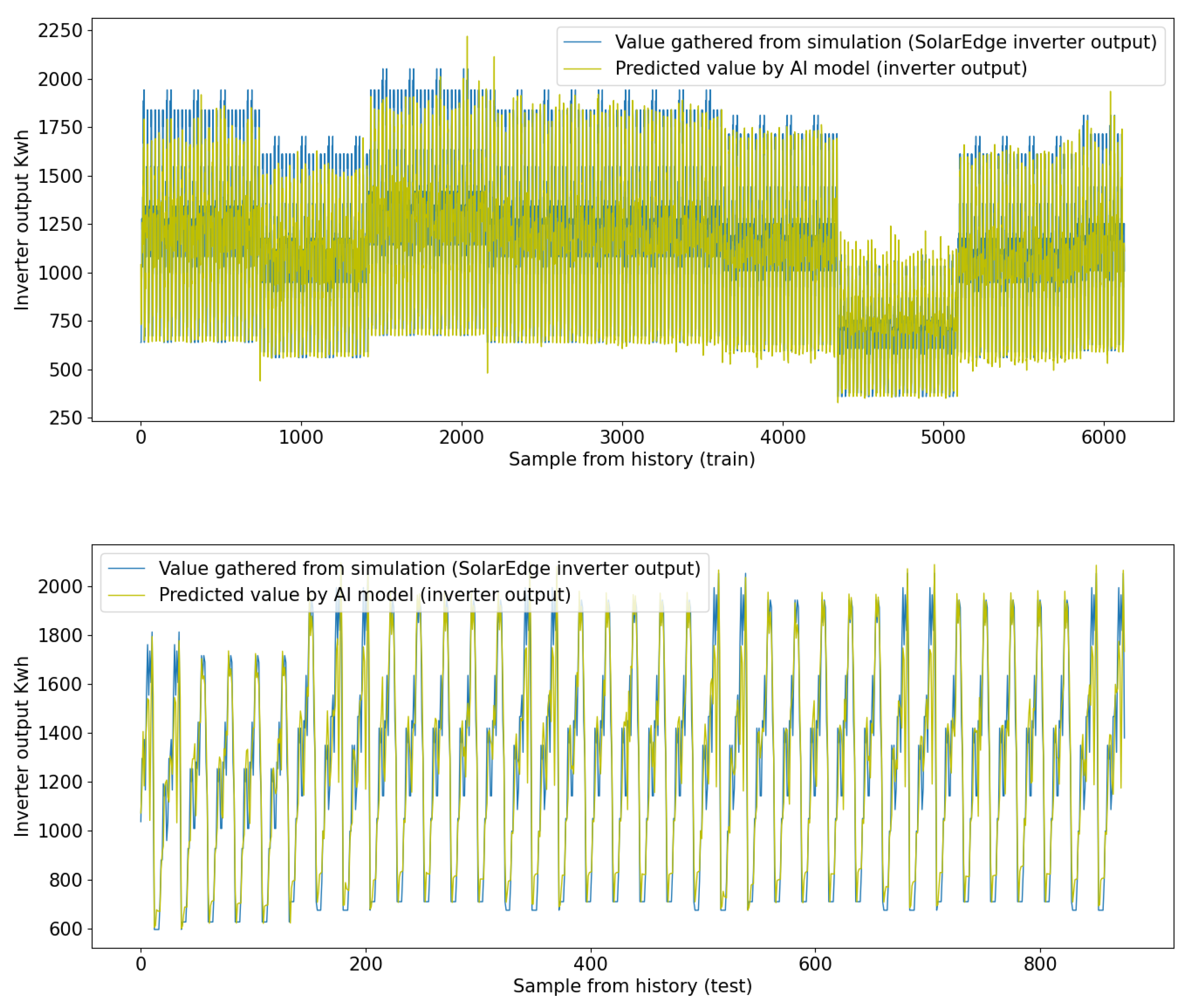
Using these parameters as input to a DNN model, it could be possible to analyze the performance of the solar PV system, predict energy output, optimize operations, and explore various scenarios for efficient energy utilization and storage.

3. Results

Below we present our comparison between values reported by simulations and our DNN models.

Based on the DNN (deep neural network) metrics provided, here is a description of most important the MultiLSTM model results (

Table 1. Metrics MultiLSTM (train).

MAE: 102.09	NMAE: 0.049	MPL: 51.0468
MAPE: 0.091	MSE: 18869.570	MAXERROR: 771.923
EVS: 0.890	R2: 0.885	RMSE: 137.366
MEAN TWEEDIE DEVIANCE: 18869.570	MEAN POISSON DEVIANCE: 16.032
MEAN GAMMA DEVIANCE 0.0147	D2 TWEEDIE SCORE: 0.885
D2 PINBALL SCORE: 0.703	D2 ABSOLUTE ERROR SCORE 0.703

and

Table 2. Metrics MultiLSTM (test).

MAE: 112.179	NMAE: 0.0546	MPL: 56.089
MAPE: 0.091	MSE: 27767.949	MAXERROR: 803.295
EVS: 0.839	R2: 0.839	RMSE: 166.637
MEAN TWEEDIE DEVIANCE: 27767.949	MEAN POISSON DEVIANCE: 21.329
MEAN GAMMA DEVIANCE 0.0172	D2 TWEEDIE SCORE: 0.839
D2 PINBALL SCORE: 0.676	D2 ABSOLUTE ERROR SCORE 0.676

):

• MAE (mean absolute error): 102.09 (train), 112.179 (test). The MAE represents the average absolute difference between the predicted values and the actual values. In this case, the average absolute error is 102.09, which means, on average, the predictions made by the DNN are off by approximately 102.09 Kwh.
• NMAE (normalized mean absolute error): 0.049 (train), 0.054 (test). NMAE is the MAE normalized by the mean of the actual values. It is a relative measure of the MAE and is useful for comparing performance across different datasets. In this case, the NMAE is 0.049, indicating that the DNN’s predictions have an average absolute error of 4.9% relative to the mean of the actual values.
• MPL (mean percentage loss): 56.089 (train/test). The MPL represents the average percentage difference between the predicted values and the actual values. In this case, the average percentage loss is 56.089, which means, on average, the predictions made by the DNN deviate from the actual values by approximately 56.089%.
• MAPE (mean absolute percentage error): 0.0918 (train/test). MAPE is a common metric for measuring the accuracy of predictions as a percentage. It represents the average absolute percentage difference between the predicted values and the actual values. In this case, the average absolute percentage error is 0.0918, meaning that the DNN’s predictions have an average error of 9.1% relative to the actual values.
• MSE (mean squared error): 18869.570 (train), 27767.949 (test). The MSE represents the average of the squared differences between the predicted values and the actual values. It gives higher weights to larger errors. In this case, the MSE is 18869.570, providing an insight into the average squared error of the DNN’s predictions.
• EVS (explained variance score): 0.890 (train), 0.839 (test). EVS measures the proportion of variance in the target variable that is explained by the model. It ranges from 0 to 1, where 1 indicates a perfect fit. An EVS of 0.889 means that the DNN explains about 89% of the variance in the data, which is considered a good result.
• R2 (R-squared): 0.885 (train), 0.839 (test). R-squared is another measure of how well the model fits the data. It represents the proportion of variance in the target variable that can be predicted from the input features. R-squared also ranges from 0 to 1, with 1 indicating a perfect fit. An R2 value of 0.885 indicates that the DNN explains about 86.7% of the variance in the data.
• RMSE (root mean squared error): 166.637 (train/test). RMSE is the square root of the MSE and is a common metric for evaluating the accuracy of predictions. It represents the average magnitude of the errors made by the DNN. In this case, the RMSE is 166.637, providing an insight into the average magnitude of the errors made by the DNN’s predictions.

Overall, the DNN seems to be performing reasonably well, with relatively low errors and high explained variance and R-squared values (Figure 7).

In this scenario, the analysis reveals the following performance metrics for the model (

Table 3. Metrics EncoderDecoder (train).

MAE: 131.257	NMAE: 0.063	MPL: 65.628
MAPE: 0.124	MSE: 31018.050	MAXERROR: 649.162
EVS: 0.814	R2: 0.812	RMSE: 176.119
MEAN TWEEDIE DEVIANCE: 31018.050	MEAN POISSON DEVIANCE: 26.525
MEAN GAMMA DEVIANCE 0.0246	D2 TWEEDIE SCORE: 0.812
D2 PINBALL SCORE: 0.618	D2 ABSOLUTE ERROR SCORE 0.618

and

Table 4. Metrics EncoderDecoder (test).

MAE: 178.811	NMAE: 0.087	MPL: 89.405
MAPE: 0.139	MSE: 50300.413	MAXERROR: 801.092
EVS: 0.745	R2: 0.709	RMSE: 224.277
MEAN TWEEDIE DEVIANCE: 50300.413	MEAN POISSON DEVIANCE: 39.998
MEAN GAMMA DEVIANCE 0.034	D2 TWEEDIE SCORE: 0.709
D2 PINBALL SCORE: 0.484	D2 ABSOLUTE ERROR SCORE 0.484

):

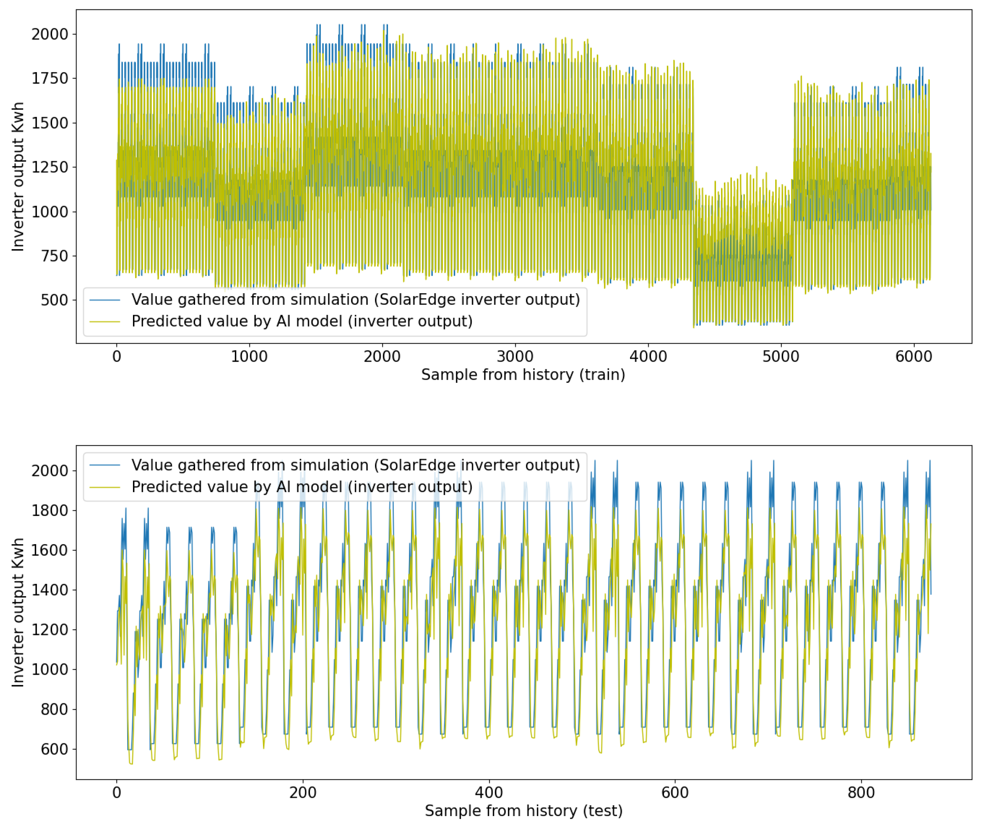
• Mean Absolute Error (MAE): The MAE is measured at approximately 131.257 Kwh (test), 178.811 KWh (train), indicating the average discrepancy between predicted and actual values.
• Normalized Mean Absolute Error (NMAE): The NMAE stands at around 0.063 (train), 0.087 (test) representing the relative average absolute error.
• Mean Absolute Percentage Error (MAPE): The MAPE is about 0.124% (train), 0.139% (test), signifying the average error as a percentage of the actual values.
• Mean Squared Error (MSE): The MSE is approximately 31018.050 (train), 50300.413 (test), reflecting the average squared difference between predicted and actual values.
• Explained Variance Score (EVS): With a value of approximately 0.814 (train), 0.745 (test), the EVS suggests a reasonably good fit of the model to the data. An EVS close to 1 indicates a stronger fit.
• Coefficient of Determination (R2): The R2 value is estimated at around 0.812 (train), 0.709 (test), which serves as a measure of the model’s accuracy in explaining the variance in the dependent variable.
• Root Mean Squared Error (RMSE): The RMSE is evaluated at approximately 176.119 KWh (train), 224.277 (test), signifying the square root of the average squared error.

EncoderDecoderLSTM model demonstrates reasonable performance within the context and specific domain of the problem (Figure 8).

4. Discussion

Emphasizing the significance of data abundance for model improvement, it becomes evident that increasing the dataset enhances output quality, particularly after applying feature selection. The accuracy of models has been assessed using R2 and NMAE metrics, with the data split into 80% for training and 20% for testing.

Choosing the best model manually can be challenging, relying solely on metrics and visual representations. To address this, an automated approach has been adopted. Leveraging benchmarks and a framework, proper hyperparameters and optimized models have been selected, considering factors like calculation costs, weight, and performance.

The automated environment presents a distinct advantage in enabling easy comparison of results. Metrics are measured for each method and learning stage, unveiling the advantages and drawbacks of different architectures. Focus on optimization aspects becomes achievable, especially when evaluating multiple horizons and methodologies. It is worth noting that the evaluation process took approximately one and a half months.

To delve into the intricacies of energy forecasting, the models’ behavior has been extensively tested concerning energy production from individual photovoltaic microinstallation based on an example from Swietokrzyskie Voivodeship Poland. This examination is based on the total energy output from micro-installation.

In conclusion, this pioneering study seeks to address the challenges posed by existing PV energy production calculation methods in Polish conditions. By identifying potential inaccuracies due to factors such as terrain, location, wind conditions, and PV panel representative characteristics, the research highlights the importance of refining these methods for more precise results.

To achieve this, the study explores the application of deep neural network (DNN) methods, with a particular focus on hybrid long short-term memory (LSTM)-based architectures. Through the evaluation of data provided by the esteemed SolarEdge simulator, the accuracy of energy production calculations can be thoroughly verified.

Moreover, this research stands as a significant milestone as it pioneers the assessment of energy production from a microinverter installation under simulated conditions in the Central Eastern European region, specifically in the Swietokrzyskie Voivodeship area. The statistical analysis conducted in this study meticulously examines the representative characteristics of the one-year analysis period, providing valuable insights into the potential of PV energy generation in this specific context.

The results of both DNN models based on R2 metrics are multi-layer LSTM R2—0.885 and EncoderDecoderLSTM R—0.812, which could let us hypothesize that using DNN models could be used for forecasting of energy production for small PV platforms.

Overall, this study’s findings and methodologies pave the way for future advancements in PV energy production calculations, fostering the development of more accurate and efficient methods tailored to the unique conditions of Poland and similar regions. With the integration of cutting-edge DNN techniques, the renewable energy industry can take a step closer to realizing its full potential in achieving a sustainable [10] and eco-friendly future.

In the future, there is a plan to use a combination of energy forecasting models and price forecasting for steering on-grid/off-grid scenarios for microinstallation in-home usage.

References

1. Demirkiran, M.; Karakaya, A. Efficiency analysis of photovoltaic systems installed in different geographical locations. Open Chem. 2022, 20, 748–758. [Google Scholar] [CrossRef]
2. Bochenek, B.; Jurasz, J.; Jaczewski, A.; Stachura, G.; Sekuła, P.; Strzyżewski, T.; Wdowikowski, M.; Figurski, M. Day-Ahead Wind Power Forecasting in Poland Based on Numerical Weather Prediction. Energies 2021, 14, 2164. [Google Scholar] [CrossRef]
3. Gołȩbiewski, D.; Barszcz, T.; Skrodzka, W.; Wojnicki, I.; Bielecki, A. A New Approach to Risk Management in the Power Industry Based on Systems Theory. Energies 2022, 15, 9003. [Google Scholar] [CrossRef]
4. Roberts, J.; Cassula, A.; Freire, J.; Prado, P. Simulation and Validation Of Photovoltaic System Performance Models. In Proceedings of the XI Latin-American Congress on Electricity Generation and Transmission–CLAGTEE 2015, Sao Paulo, Brazil, 8–11 November 2015. [Google Scholar]
5. Milosavljević, D.D.; Kevkić, T.S.; Jovanović, S.J. Review and validation of photovoltaic solar simulation tools/software based on case study. Open Phys. 2022, 20, 431–451. [Google Scholar] [CrossRef]
6. Shao, X.; Kim, C.-S.; Sontakke, P. Accurate Deep Model for Electricity Consumption Forecasting Using Multi-Channel and Multi-Scale Feature Fusion CNN–LSTM. Energies 2020, 13, 1881. [Google Scholar] [CrossRef]
7. Ma, H.; Xu, L.; Javaheri, Z.; Moghadamnejad, N.; Abedi, M. Reducing the consumption of household systems using hybrid deep learning techniques. Sustain. Comput. Inform. Syst. 2023, 38, 100874. [Google Scholar] [CrossRef]
8. Wang, B.; Wang, X.; Wang, N.; Javaheri, Z.; Moghadamnejad, N.; Abedi, M. Machine learning optimization model for reducing the electricity loads in residential energy forecasting. Sustain. Comput. Inform. Syst. 2023, 38, 100876. [Google Scholar] [CrossRef]
9. Bilski, J.; Rutkowski, L.; Smolag, J.; Tao, D. A novel method for speed training acceleration of recurrent neural networks. Inf. Sci. 2021, 553, 266–279. [Google Scholar] [CrossRef]
10. Wąs, K.; Radoń, J.; Sadłowska-Sałęga, A. Thermal Comfort—Case Study in a Lightweight Passive House. Energies 2022, 15, 4687. [Google Scholar] [CrossRef]
Figure 1. Microinstallation parameters.
Energies 16 06632 g001
Figure 2. Estimated monthly energy production.
Energies 16 06632 g002
Figure 3. Proposed localization of PV panels on real location bird view and leveling, Azimuth 145, slope 10.
Energies 16 06632 g003
Figure 4. Three mppt strings connection between PV panels.
Energies 16 06632 g004
Figure 5. MultiLSTM DNN model architecture.
Energies 16 06632 g005
Figure 6. EncoderDecoder DNN model architecture.
Energies 16 06632 g006
Figure 7. MultiLSTM comparison results of inverted output power simulation vs. DNN model.
Energies 16 06632 g007
Figure 8. EncoderDecoderLSTM comparison results of inverted output power simulation vs. DNN model.
Energies 16 06632 g008