Modeling and Nonlinear Characteristics Analysis of Fluorescent Lamp Driven by a Full-Bridge Inverter

Abstract

Addressing the issue of system stability is a crucial step towards the successful integration of memristive devices in power electronics applications. This paper focuses on fluorescent lamps possessing memristive characteristics and investigates the instability phenomena and mechanisms within a full-bridge inverter with a fluorescent lamp load. Based on the memristive characteristics of fluorescent lamps, this paper establishes the averaged model of the system, whose coefficient matrix is nonlinear, periodic, and time-varying. This study identifies the occurrence of low-frequency oscillations within the system and elucidates the fundamental mechanism underlying the emergence of low-frequency oscillations. Furthermore, this paper establishes the stability boundaries of the system across different parameter planes. The research findings indicate that the low-frequency oscillations within the system are attributed to the occurrence of Hopf bifurcations in a frequency range higher than line frequency but significantly lower than switching frequency. Lastly, the PSpice circuit of the system is designed, and simulation results are provided for validation. This study can offer guidance on parameters and control strategies for ensuring the stable operation of a full-bridge inverter with fluorescent lamps. Moreover, it can facilitate the comprehension of instability mechanisms in systems incorporating memristive devices, thereby offering a foundation for the expansion of memristor applications.

1. Introduction

In 1971, according to the symmetry and completeness principle of circuit theory, Chua LO proposed the concept of the memristor, which describes the relationship between the charge and the magnetic flux and is called the fourth basic circuit element [1]. The proposal of the memristor concept increased the number of fundamental circuit elements from three to four, thereby enriching and completing the theoretical framework of circuit theory. Moreover, Chua LO has expanded and refined the concept of the memristor. He classified all memristors into three classes called ideal, Generic, or Extended memristors [2,3,4]. However, despite the proposal of the memristor concept, progress in the corresponding research was hindered by the absence of a physical entity. Until 2008, HP LABS successfully manufactured solid-state memristor devices based on nanoscale TiO₂ [5]. Since then, the study of memristors and memristive systems has attracted more and more attention, resulting in a wealth of research achievements documented in the open literature. For example, Ventra MD extended the concept of memristors to include meminductors and memcapacitors [6]. On this basis, Yin Z Y provided a more detailed explanation of the memristor, meminductor, and memcapacitor [7]. Biolek Z studied the mechanism of the hysteretic curve of the memristor [8] and proposed the method for calculating the area in the hysteretic curve of the memristor, which proved that the area of the pinched hysteresis loop of the current-controlled ideal memristor represents the quantity “content” introduced into the theory of nonlinear systems by Millar in 1951 [9,10]. In addition, according to the results on fluorescent lamps in the literature [11], it can be seen that fluorescent lamps show the obvious memristor’s characteristics, which arouse people’s interest. For example, based on the theoretical analysis of low-pressure discharge in the positive column region and the Francis equation, Dai Guojun proposed a PSpice model of a fluorescent lamp [12]. Based on gas discharge theory, Wei Yan established a semi-theoretical model of a fluorescent lamp that fully accords with the definition of a fluid-controlled memristor. The model can predict the electrical characteristics of different types of fluorescent lamps at different operating frequencies and different dimming levels [13]. On the basis of the literature [13], D. Lin used a unified mathematical framework to build mathematical models of high-pressure and low-pressure gas discharge lamps and pointed out that both high-pressure and low-pressure gas discharge lamps have memristor characteristics [14]. Based on [14], S. P. Adhikari briefly analyzed the non-crossing characteristics of the hysteresis loops of fluorescent lamps at the origin [15].

Moreover, a considerable number of electrical devices have been experimentally identified as belonging to the category of memristive systems. These devices include; however, are not limited to, thermistors, tungsten filament lamps, current-controlled discharge tubes, and first-generation radio detectors [2,16,17]. Additionally, certain commonly encountered circuit systems have exhibited memristive characteristics in their external behavior during energization. For instance, in a significant study conducted in 2012, Corinto and Ascoli demonstrated that a diode bridge post-connected with an LCR filter can manifest memristive external characteristics, leading to its designation as a memristive diode bridge circuit [18]. It is foreseeable that in the future, an increasing number of electrical devices exhibiting memristive characteristics will be discovered or manufactured. Memristive electrical devices require operating in an alternating current environment devoid of direct current bias. The inverter circuits are power electronic conversion circuits capable of converting DC to AC power and serve as vital power sources for memristive electrical devices. Due to the transitions between different states of the power switches, the inverter itself operates as a segmented circuit, exhibiting intricate nonlinear phenomena.

Currently, research on complex nonlinear phenomena in inverters has become widespread. In 2002, Robert et al. first extended the study of nonlinear complex behaviors to the realm of DC/AC converters, analyzing boundary-collision bifurcations and chaos phenomena in single-phase H-bridge inverters [19]. In 2006, Kousaka et al. conducted an analysis of period orbit stability in single-phase H-bridge inverters using the return map method. By using this map, the stability of the periodic orbit can be analyzed simply using the symbolic sequence [20]. In 2009, Wang et al. established a first-order discrete model through iterative techniques and employed frequency-flashing mapping, folding mapping, and bifurcation mapping to describe bifurcation and chaos phenomena in proportional control single-phase H-bridge inverter systems [21,22]. In 2012, Wu et al. proposed control methods for fast-scale and slow-scale bifurcations in voltage-controlled H-bridge inverter circuits from a frequency-domain perspective [23]. In 2013, Liu et al. investigated the symmetric phenomena of fast-scale bifurcations in peak current and valley current-controlled H-bridge inverter circuits. The simulation showed that the symmetrical dynamical phenomenon occurs in the single-phase H-bridge inverter controlled by the peak current or the valley current [24]. In 2016, Zhang et al. proposed an improved averaging modeling method and analyzed the fast-scale bifurcation behavior in peak current-controlled Buck-Boost inverters. This method can increase the resolution of the conventional classic averaged model by half the switching frequency [25]. However, despite the significant body of research in this area, it is worth noting that the majority of the aforementioned studies have predominantly concentrated on linear loads, and the stability analysis of inverters with memristive loads has not been extensively explored. Existing research findings have demonstrated that memristive loads have a certain impact on the dynamic characteristics of power electronic circuits [26,27,28]. Due to the nonlinear characteristics of memristors, the full-bridge inverter with memristive loads exhibits nonlinearity during the periods of power switching on and off, indicating that it is a piecewise nonlinear system. Furthermore, in comparison with inverters having linear loads, the memristive nature of memristors leads to an increase in the system’s order. This complexity contributes to a range of nonlinear behaviors and challenges, thus amplifying the intricacy and difficulty of system parameter design. Some investigations have resorted to approximating memristive loads as linear loads for the sake of simplicity [29]. Such oversimplified approaches inevitably overlook the intricate and unique characteristics inherent in inverters with memristive loads, thereby hindering their ability to provide comprehensive guidance for the precise design and optimization of these specialized systems.

Therefore, the stable operation of inverters with memristive loads becomes a pivotal foundation driving the advancement and application of memristors and is poised to emerge as a crucial issue in the future. Fluorescent lamps, as the most common memristive electrical devices, exhibit significant representativeness. In practical applications, an inverter supplies high-frequency AC power to fluorescent lamps to drive their stable operation [30]. However, both fluorescent lamps and inverters are strong nonlinear systems, leading to the full-bridge inverter with the fluorescent lamp being a class of strongly nonlinear systems in which there must be a wealth of complex nonlinear phenomena, such as bifurcation, chaos, and so on, leading to greater noise and instability, not conducive to practical engineering applications. Therefore, a comprehensive investigation into the nonlinear dynamic behavior of the inverter with a fluorescent lamp load not only serves as a valuable reference for better comprehension and enhancement of system design but also contributes to the advancement of memristive device applications in power electronic circuits.

Addressing the aforementioned issues and limitations, this paper establishes a mathematical model for a full-bridge inverter system with a fluorescent lamp, taking into account the memristive characteristics of the fluorescent lamp. Through Matlab/Simulink simulations, we identify the presence of low-frequency oscillations in the system. Employing the harmonic balance method and Floquet theory, it elucidates the fundamental mechanism of these oscillations and outlines the system’s stability boundaries across various parameter planes. Furthermore, a PSpice simulation model is constructed, yielding results consistent with theoretical analysis, thus validating the accuracy of the theoretical insights.

2. Mathematical Modeling and Simulations

In 2007, Wei Yan et al. established the mathematical model of a fluorescent lamp through experiments and a genetic algorithm [14], namely

$$\{\begin{array}{l}u=M(T)i\\ M(T)=a_5{T}^{-\frac{3}{4}}\exp (\frac{e{a}_6}{2kT})\\ \frac{dT}{dt}=a_1[M(T)i^2-a_4(T-T_0)-a_2\exp (\frac{-e{a}_3}{kT})]\end{array}$$

(1)

where t is the time, e is the charge on the electron, and e = 1.6 × 10⁻¹⁹ C, k is the Boltzmann constant, and k = 1.38 × 10⁻²³ J/K, T is the electron temperature, and the initial value of T is $T_0$ = 350 K, and a₁–a₆ are the adjustable model coefficients.

Based on the classification of memristors in Ref. [31], the mathematical model of a fluorescent lamp conforms to the constitutive relation of a current-controlled memristor, whose memristor value is

$$M=a_5{T}^{-\frac{3}{4}}\exp (\frac{e{a}_6}{2kT})$$

(2)

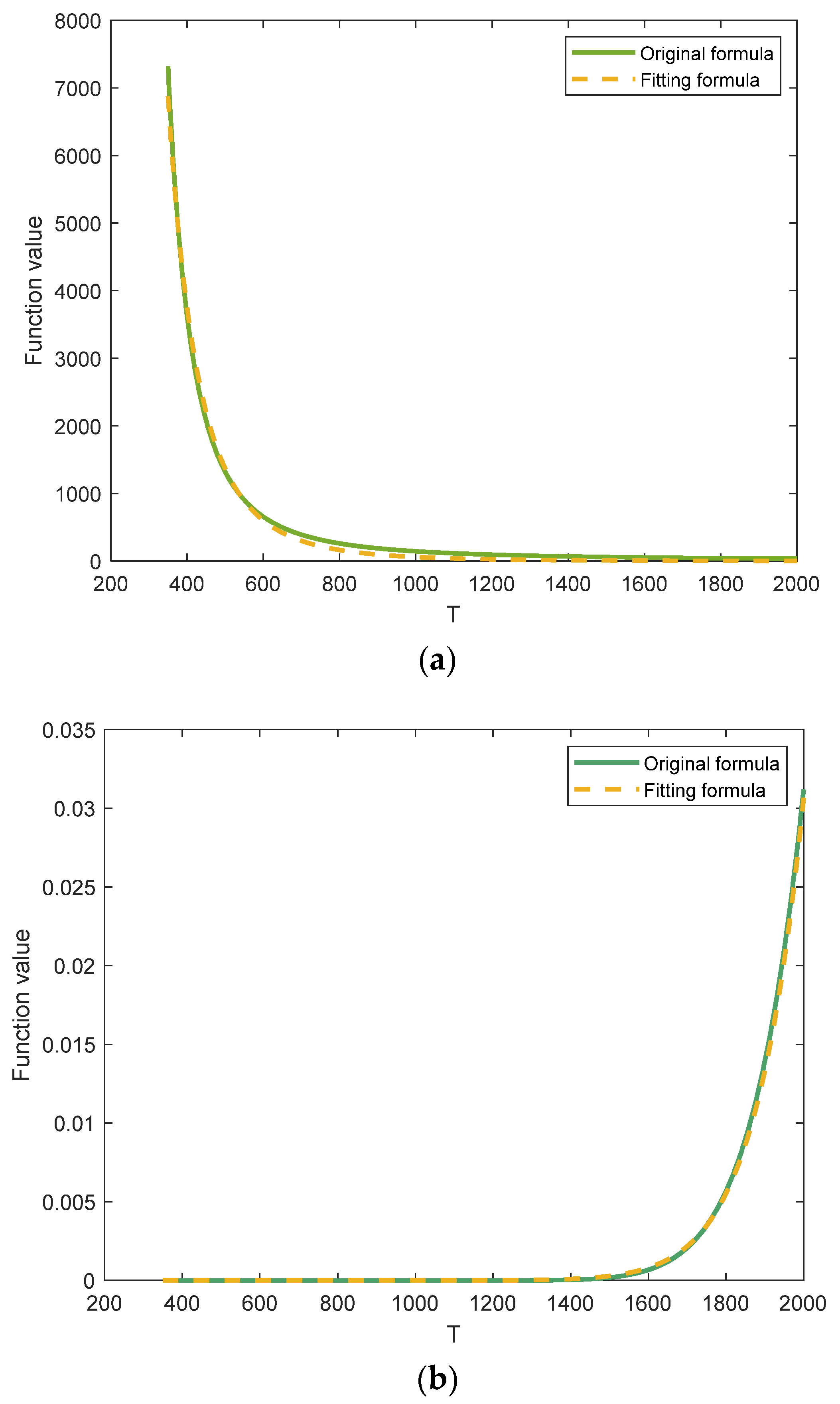
The second and third expressions of (1) are transcendental functions with respect to T, which will bring difficulties to theoretical calculation and analysis. Here, according to the model parameters given in Ref. [15], the approximate fitting is performed on equations a₅T^−0.75exp(ea₆/(2kT)) and a₂exp(−ea₃/(kT)). That is,

$$\{\begin{array}{l}{a}_5{T}^{-0.75}\exp (\frac{e{a}_6}{2kT})\approx 2.145\times {10}^{15}\cdot T^{-4.518}\\ a_2\exp (\frac{-e{a}_3}{kT})\approx 5.569\times {10}^{-56}·T^{16.28}\end{array}$$

(3)

As can be seen from Figure 1, the fitting R-square of a₅T^−0.75exp(ea₆/(2kT)) is 0.9944, and the fitting R-square of a₂exp(−ea₃/(kT)) is 0.9998, which shows that the fitting accuracy is very high. Thus, it is effective to use the simplified model instead of a₅T^−0.75exp(ea₆/(2kT)) and a₂exp(−ea₃/(kT)).

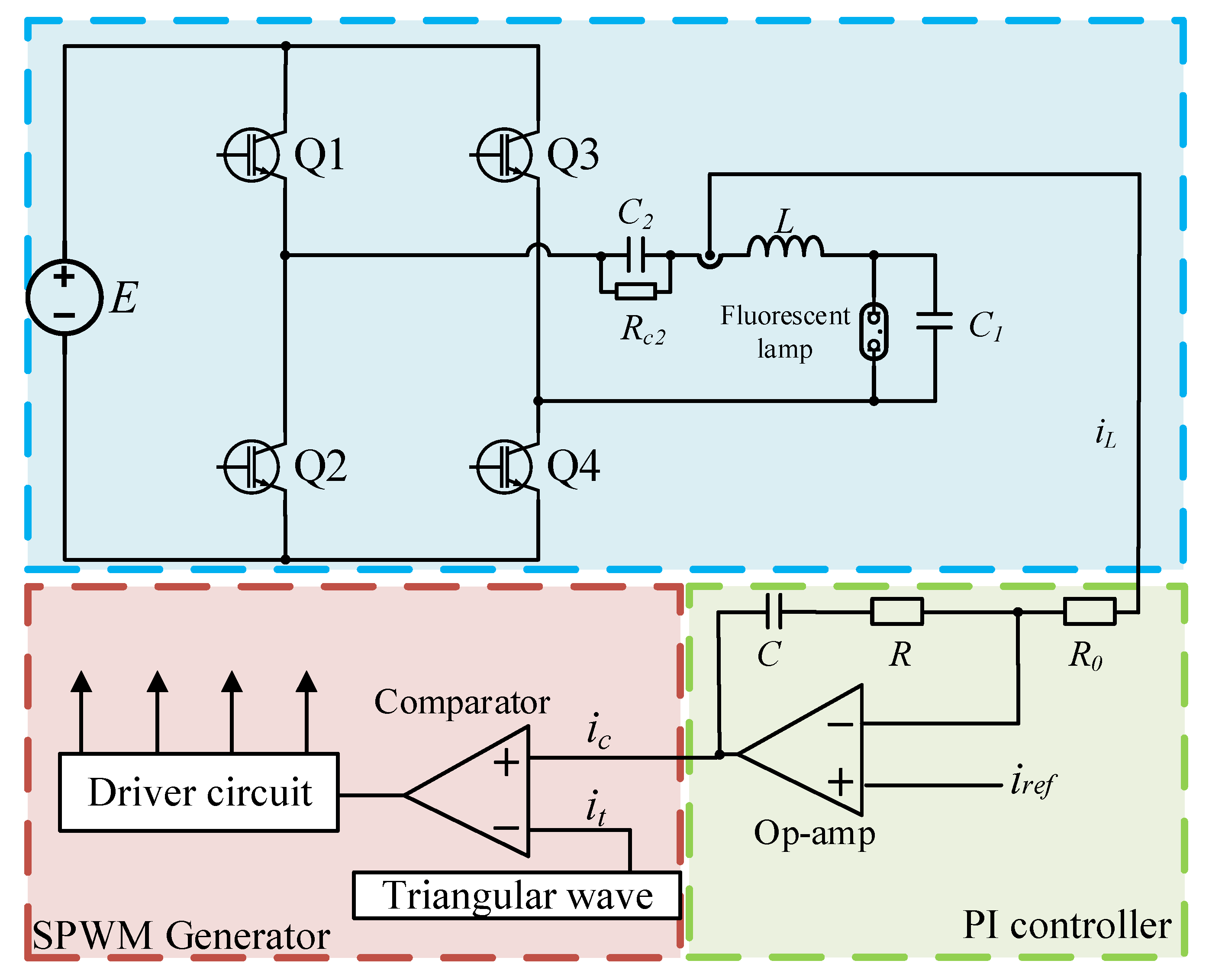
Generally speaking, the operational frequency of fluorescent lamps typically ranges from 20 kHz to 100 kHz. A high-frequency AC power supply enables fluorescent lamps to produce more stable and uniform illumination, thereby reducing visible flickering. In electronic ballasts, the high-frequency AC power is generated by the inverter circuit. Therefore, the inverter is the most basic and critical component of the electronic ballast, and the full-bridge inverter is one of the most common topologies. Therefore, here, the PI current feedback-controlled full-bridge inverter is used to drive a fluorescent lamp as the research object, and its circuit model is shown in Figure 2. This circuit is mainly composed of the DC voltage source E, power switches Q1~Q4, LCC (LCC is a circuit topology consisting of an inductor and two capacitors, hence its name LCC) branch, the fluorescent lamp load, and the current feedback controller. The control section adopts the SPWM (Sinusoidal Pulse Width Modulation) current control mode, where the output current i_L is compared with the reference current i_ref. The error signal resulting from this comparison is fed into a PI controller to obtain the modulating signal i_c. This modulating signal i_c is then compared with a triangular wave i_t to generate a driving signal, which is used to control the on-off of the power switches. When the driving signal is high, the corresponding power switches are on; otherwise, they are off. Note that Q1 and Q4 have the same drive signals, as do Q2 and Q3. Note that the insulation resistance R_c2 of capacitor C₂ is considered (note: R_c2 stands for loss in the dielectric, and R_c2 is usually large, generally above 1 MΩ [32,33]).

The bipolar SPWM generator in Figure 2 consists of a COM (Comparator), a triangular carrier i_t, and a power switch driver. Note that the chosen operating frequency f₀ for the fluorescent lamp is f₀ = 25 kHz, which results in ω₀ = 2πf₀ = 50,000π, And the triangular carrier i_t and reference current i_ref are presented as follows:

$$i_t=\{\begin{array}{l}({\omega }_{sw}t-2\pi k)\frac{2I_{tri}}{\pi }-I_{tri}, 2\pi k<{\omega }_{sw}t<2\pi k+\pi \\ -({\omega }_{sw}t-2\pi k-2\pi )\frac{2I_{tri}}{\pi }-I_{tri}, 2\pi k+\pi \le {\omega }_{sw}t\le 2\pi k+2\pi \end{array}$$

(4)

$$i_{ref}=I_{ref}\sin ({\omega }_{0}t)$$

(5)

where ${\omega }_{sw}$ and $I_{tri}$ are the angular frequency and amplitude of the triangular carrier respectively.

If

i_t < i_c

(6)

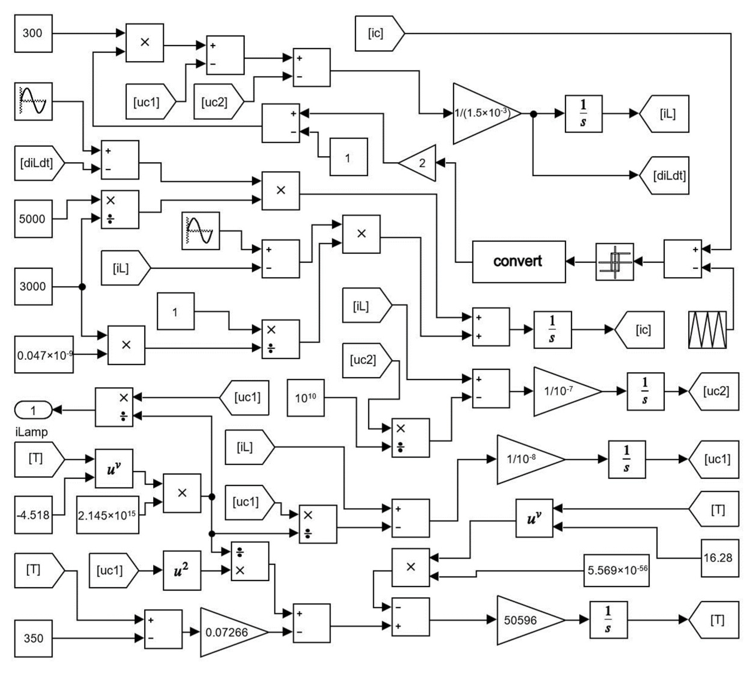
The output of a comparator is high; otherwise, it is low. According to KCL (Kirchhoff’s Current Law) and KVL (Kirchhoff’s Voltage Law) [34], the mathematical model of the system described by the differential equation can be derived as follows:

$$\{\begin{array}{l}\frac{d{i}_L}{dt}=\frac{1}{L}((2S-1)E-u_{C1}-u_{C2})\\ \frac{d{u}_{C1}}{dt}=\frac{1}{C_1}(i_L-\frac{u_{C1}\cdot T^{4.518}}{2.145\times {10}^{15}})\\ \frac{d{u}_{C2}}{dt}=\frac{1}{C_2}(i_L-\frac{u_{C2}}{R_{C2}})\\ \frac{dT}{dt}=a_1(\frac{T^{4.518}\cdot u_{C1}{}^2}{2.145\times {10}^{15}}-a_4(T-T_0)-5.569\times {10}^{-56}\cdot T^{16.28})\\ \frac{d{i}_c}{dt}=-k_p\frac{d{i}_L}{dt}-k_i{i}_L+k_p{I}_{ref}{\omega }_0\cos ({\omega }_{0}t)+k_i{I}_{ref}\sin ({\omega }_{0}t)\end{array}$$

(7)

When S = 1, means Q1 and Q4 are turned on, and Q2 and Q3 are turned off. On the contrary, Q2 and Q3 are turned on, and Q1 and Q4 are turned off. According to Formula (5), the MATLAB/Simulink simulation model of the full-bridge inverter system with the fluorescent lamp is established, as shown in Figure 3. As indicated by Equation (5) and Figure 3 in the original manuscript, it can be observed that when a fluorescent lamp is connected, compared to an inverter with a linear load, the memristive nature of the lamp leads to an increase in the system’s order. Usually, power electronic systems can be regarded as segmented linear switching circuits. However, due to the memristive characteristics of fluorescent lamps, the full-bridge inverter with fluorescent lamps exhibits nonlinearity during the periods of power switching on and off. In other words, the full-bridge inverter with fluorescent lamp is a segmented nonlinear system that is more complicated and more prone to generating oscillations and other nonlinear behaviors.

In actual electronic ballasts, the amplitude of the rectified DC voltage is around 300 V; hence, we opted for E = 300 V. The inductance L of the LCC branch is on the order of millihenries (mH), while both C₁ and C₂ have values in the nanofarad (nF) range. The electronic ballast achieves high-voltage ignition of the fluorescent lamp through the resonance of the LCC branch. The resonance frequency for ignition (f_res1) should be higher than the operating frequency of the fluorescent lamp. And to ensure that the LCC branch operates in an inductive state, the operating frequency of the fluorescent lamp needs to be higher than the steady-state resonance frequency (f_res2).

$$f_{res1}=\frac{1}{2\pi }\sqrt{\frac{C_1+C_2}{L{C}_1{C}_2}}>25000$$

(8)

$$f_{res2}=\frac{1}{2\pi \sqrt{L{C}_2}}<25000$$

(9)

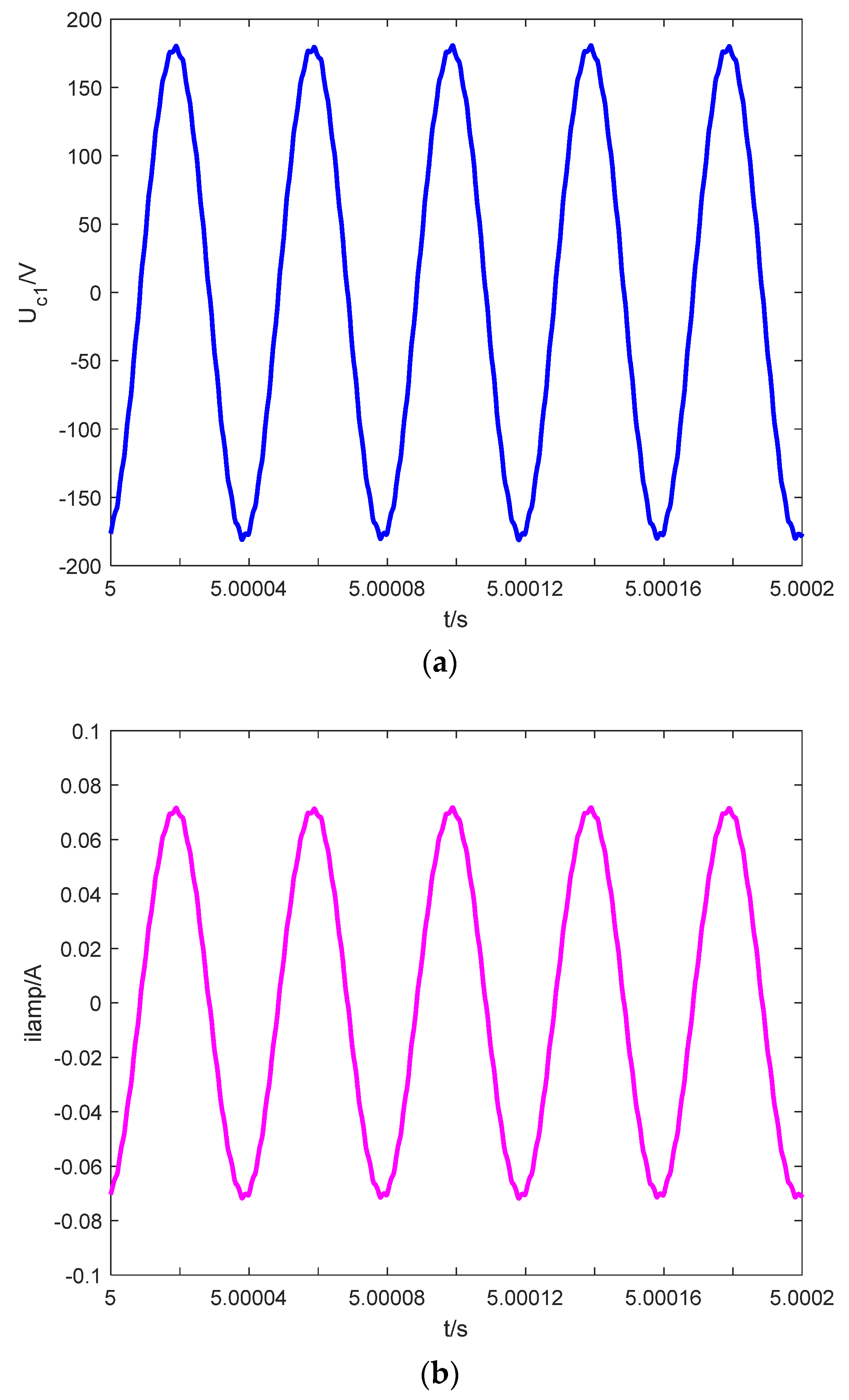
Choosing C₁ = 10 nF, C₂ = 100 nF, and L = 1.5 mH can meet the requirements. The other circuit parameters are selected as I_ref = 0.3 V, C = 0.047 nF, R₀ = 3 kΩ, I_tri = 1 V.

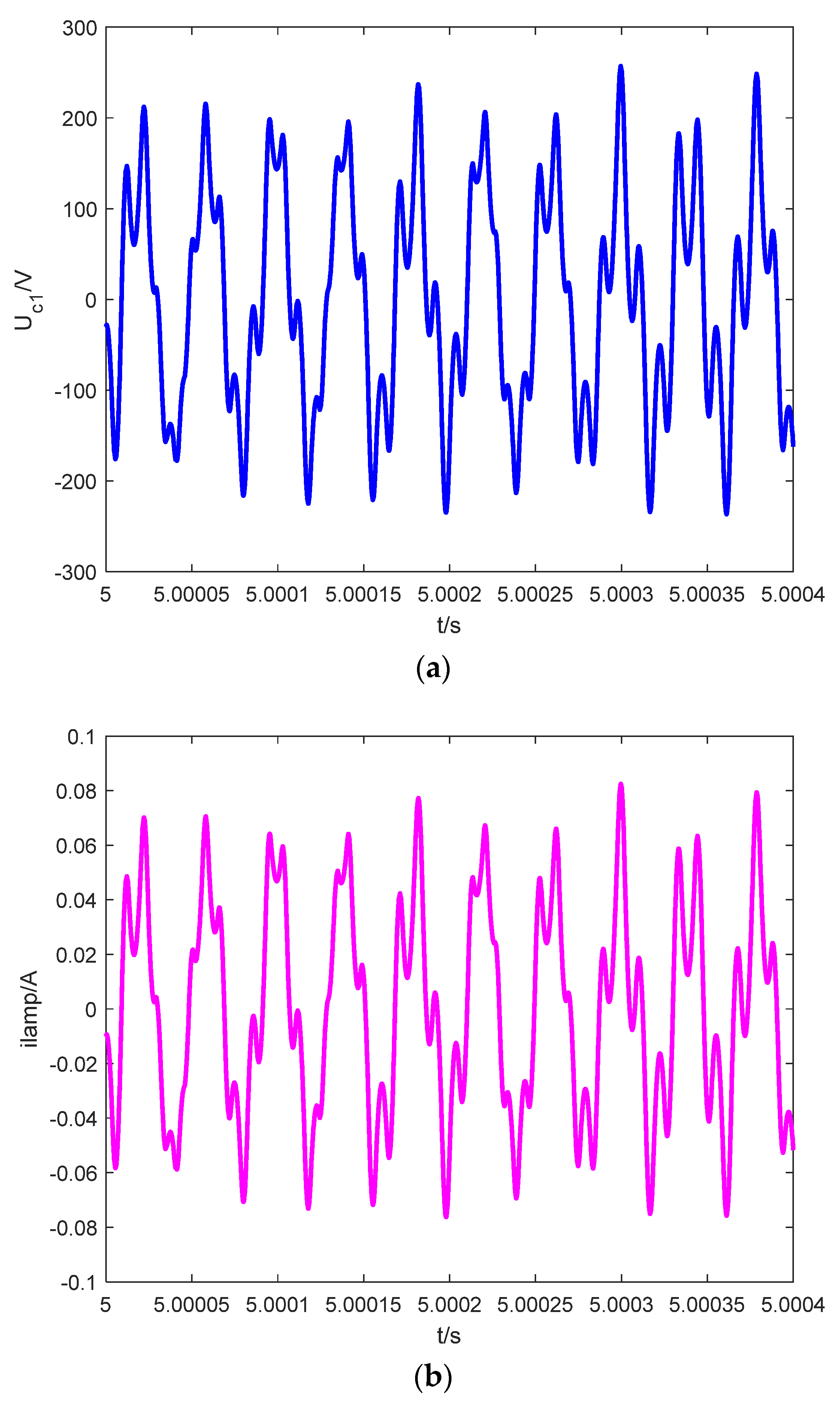
Figure 4 shows the Matlab/Simulink simulation results under R = 5 kΩ. In Figure 4a, U_c1 is the time-domain waveform of the voltage across the fluorescent lamp, while Figure 4b is the time-domain waveform of the current through the fluorescent lamp. From Figure 4, it is obvious that the system is in stable operation. However, the system is unstable and in a state of low-frequency oscillation when R = 50 Ω, which is shown in Figure 5. Obviously, the resistance R has an important effect on the occurrence of low-frequency oscillation in the fluorescent lamp system driven by the full bridge inverter.

3. Analysis of Low-Frequency Oscillation Mechanism of the System

Firstly, the approximate solution of a full-bridge inverter with a fluorescent lamp is obtained by the harmonic balance method. Then, the Floquet theory is used to identify the mechanism responsible for the occurrence of low-frequency oscillation.

3.1. Approximate Solution

Since the angular frequency of the triangular carrier i_t is much larger than that of the modulated wave, the switching frequency is much larger than that of the modulated wave’s frequency. Therefore, based on the average modeling method of power electronic systems [35], the average model of the system can be established, and the expression of the duty cycle $\langle d\rangle$ is

$$\langle d\rangle =\frac{1}{2}(1+\frac{\langle i_c\rangle }{I_{tri}})$$

(10)

By substituting $\langle d\rangle$ for the term S in the first formula of Equation (7), the average model of the full-bridge inverter with fluorescent lamp controlled by PI current feedback control can be established as

$$\{\begin{array}{l}\frac{d\langle i_L\rangle }{dt}=\frac{1}{L}(\frac{\langle i_c\rangle }{I_{tri}}E-\langle u_{C1}\rangle -\langle u_{C2}\rangle )\\ \frac{d\langle u_{C1}\rangle }{dt}=\frac{1}{C_1}(\langle i_L\rangle -\frac{\langle u_{C1}\rangle {\langle T\rangle }^{4.518}}{2.145\times {10}^{15}})\\ \frac{d\langle u_{C2}\rangle }{dt}=\frac{1}{C_2}(\langle i_L\rangle -\frac{\langle u_{C2}\rangle }{R_{C2}})\\ \frac{d\langle T\rangle }{dt}=a_1(\frac{{\langle T\rangle }^{4.518}{\langle u_{C1}\rangle }^2}{2.145\times {10}^{15}}-a_4(\langle T\rangle -T_0)-5.569\times {10}^{-56}{\langle T\rangle }^{16.28})\\ \frac{d\langle i_c\rangle }{dt}=-k_p\frac{1}{L}(\frac{\langle i_c\rangle }{I_{tri}}E-\langle u_{C1}\rangle -\langle u_{C2}\rangle )-k_i\langle i_L\rangle +k_p{I}_{ref}{\omega }_0\cos ({\omega }_{0}t)+k_i{I}_{ref}\sin ({\omega }_{0}t)\end{array}$$

(11)

where, $\langle i_L\rangle$, $\langle i_c\rangle$, $\langle u_{C1}\rangle$ and $\langle T\rangle$ are respectively the average values of $i_L$, $i_c$, $u_{C1}$ and $T$ in a switching cycle.

It can be seen that the current mode-controlled full-bridge inverter with fluorescent lamp described in (11) is a nonlinear and non-autonomous system. Equation (11) involves five variables. In order to obtain the approximate solution of the full-bridge inverter with a fluorescent lamp, it is necessary to reduce the number of variables through equation manipulation. By combining the first, third, and fifth formulas of Equation (11), the variables $\langle u_{C2}\rangle$ and $\langle i_c\rangle$ can be eliminated. The specific process is as follows:

From the first formula of (11), we can obtain

$$\langle i_c\rangle =\frac{I_{tri}}{E}(L\langle i_{{}_L}^{\prime }\rangle +\langle u_{C1}\rangle +\langle u_{C2}\rangle )$$

(12)

After differentiating both sides of (12) with respect to time t, we can obtain

$$\langle i_{{}_c}^{\prime }\rangle =\frac{I_{tri}}{E}(L\langle i_{{}_L}^{\prime \prime }\rangle +\langle u_{{}_{C1}}^{\prime }\rangle +\langle u_{{}_{C2}}^{\prime }\rangle )$$

(13)

After substituting the third expression of (11) into (13), the variable $\langle u_{C2}\rangle$ can be eliminated, resulting in

$$\langle i_{{}_c}^{\prime }\rangle =\frac{I_{tri}}{E}(L\langle i_{{}_L}^{\prime \prime }\rangle +\langle u_{{}_{C1}}^{\prime }\rangle +\frac{\langle i_L\rangle }{C_2}-\frac{1}{C_2\cdot R_{C2}}\exp (-\frac{t}{C_2\cdot R_{C2}})({\displaystyle \int \frac{\langle i_L\rangle }{C_2}\cdot \exp (\frac{t}{C_2\cdot R_{C2}})dt}))$$

(14)

where, $\exp$ is the exponential function.

By combining the fifth formula of (11) with (14), the variable $\langle i_c\rangle$ can be eliminated. we can obtain

$$\begin{array}{l}-k_p\langle i_L^{\prime }\rangle -k_i\langle i_L\rangle +k_p{I}_{ref}{\omega }_0\cos ({\omega }_{0}t)+k_i{I}_{ref}\sin ({\omega }_{0}t)=\\ \frac{I_{tri}}{E}(L\langle i_L^{″}\rangle +\frac{1}{C_2}\langle i_L\rangle +\langle u_{C1}^{\prime }\rangle -\frac{1}{C_2\cdot R_{C2}}\exp (-\frac{t}{C_2\cdot R_{C2}}){\displaystyle \int \frac{\langle i_L\rangle }{C_2}\exp (\frac{t}{C_2\cdot R_{C2}})dt})\end{array}$$

(15)

Equation (15) contains only the variables $\langle i_L\rangle$ and $\langle u_{C1}\rangle$, as well as their differentials and integrals, which can be abbreviated as

$$l(i_L^{\prime },i_L)=g(i_L^{\prime \prime },i_L,u_{C1}^{\prime })$$

(16)

where,

$$l(i_L^{\prime },i_L)=-k_p\langle i_L^{\prime }\rangle -k_i\langle i_L\rangle +k_p{I}_{ref}{\omega }_0\cos ({\omega }_{0}t)+k_i{I}_{ref}\sin ({\omega }_{0}t)$$

(17)

$$\begin{array}{l}g(i_L^{″},i_L,u_{C1}^{\prime })=\frac{I_{tri}}{E}(L\langle i_L^{″}\rangle +\frac{1}{C_2}\langle i_L\rangle +\langle u_{C1}^{\prime }\rangle \\ -\frac{1}{C_2\cdot R_{C2}}\exp (-\frac{t}{C_2\cdot R_{C2}}){\displaystyle \int \frac{\langle i_L\rangle }{C_2}\exp (\frac{t}{C_2\cdot R_{C2}})dt})\end{array}$$

(18)

By combining the second and fourth formulas of Equation (11), the variables $\langle T\rangle$ can be eliminated. The specific process is as follows:

From the second formula of (11), we can obtain

$$\langle T\rangle =2474.1(\frac{\langle i_L\rangle -C_1\langle u^{\prime }{}_{C1}\rangle }{\langle u_{C1}\rangle }{)}^{0.2213}$$

(19)

After differentiating both sides of (19) with respect to time t, we can obtain

$$\begin{array}{l}\langle T^{\prime }\rangle =547.6(\frac{\langle i_L^{\prime }\rangle \langle u_{C1}\rangle -\langle u_{C1}^{\prime }\rangle \langle i_L\rangle }{\langle u_{C1}^2\rangle }\\ -C_1\frac{\langle u_{C1}^{\prime \prime }\rangle \langle u_{C1}\rangle -\langle u_{C1}^{\prime }\rangle \langle u_{C1}^{\prime }\rangle }{\langle u_{C1}^2\rangle })(\frac{\langle i_L\rangle -C_1\langle u^{\prime }{}_{C1}\rangle }{\langle u_{C1}\rangle }{)}^{-0.7786}\end{array}$$

(20)

By combining (19), (20), and the fourth formula of (11), we can obtain

$$\begin{array}{l}547.6(\frac{\langle i_L^{\prime }\rangle \langle u_{C1}\rangle -\langle u_{C1}^{\prime }\rangle \langle i_L\rangle }{\langle u_{C1}^2\rangle }-C_1\frac{\langle u_{C1}^{\prime \prime }\rangle \langle u_{C1}\rangle -\langle u_{C1}^{\prime }\rangle \langle u_{C1}^{\prime }\rangle }{\langle u_{C1}^2\rangle })(\frac{\langle i_L\rangle -C_1\langle u^{\prime }{}_{C1}\rangle }{\langle u_{C1}\rangle }{)}^{-0.7786}=\\ a_1(\langle u_{{}_{C1}}\rangle (\langle i_{{}_L}\rangle -C_1\langle u_{C1}^{\prime }\rangle )-a_{{}_4}(2474.1(\frac{\langle i_L\rangle -C_1\langle u^{\prime }{}_{C1}\rangle }{\langle u_{C1}\rangle }{)}^{0.2213}-350)\\ -0.9784(\frac{\langle i_{{}_L}\rangle -C1\langle u_{C1}^{\prime }\rangle }{\langle u_{{}_{C1}}\rangle }{)}^{3.6034})\end{array}$$

(21)

Equation (15) contains only the variables $\langle i_L\rangle$ and $\langle u_{C1}\rangle$, as well as their differentials, which can be abbreviated as

$$p(i_L^{\prime },i_L,u_{C1}^{\prime \prime },u_{C1}^{\prime },u_{C1})=q(i_L^{\prime },i_L,u_{C1}^{\prime },u_{C1})$$

(22)

where,

$$\begin{array}{l}p(i_L^{\prime },i_L,u_{C1}^{″},u_{C1}^{\prime },u_{C1})=547.6(\frac{\langle i_L^{\prime }\rangle \langle u_{C1}\rangle -\langle u_{C1}^{\prime }\rangle \langle i_L\rangle }{\langle u_{C1}^2\rangle }\\ -C_1\frac{\langle u_{C1}^{\prime \prime }\rangle \langle u_{C1}\rangle -\langle u_{C1}^{\prime }\rangle \langle u_{C1}^{\prime }\rangle }{\langle u_{C1}^2\rangle }){(\frac{(\langle i_L\rangle -C_1\langle u^{\prime }{}_{C1}\rangle )}{\langle u_{C1}\rangle })}^{-0.7786}\end{array}$$

(23)

$$\begin{array}{l}q(i_L^{\prime },i_L,u_{C1}^{\prime },u_{C1})=a_1(\langle u_{{}_{C1}}\rangle (\langle i_{{}_L}\rangle -C_1\langle u_{C1}^{\prime }\rangle )\\ -a_{{}_4}(2474.1(\frac{\langle i_L\rangle -C_1\langle u^{\prime }{}_{C1}\rangle }{\langle u_{C1}\rangle }{)}^{0.2213}-350)-0.9784(\frac{\langle i_{{}_L}\rangle -C1\langle u_{C1}^{\prime }\rangle }{\langle u_{C1}\rangle }{)}^{3.6034})\end{array}$$

(24)

For this system, the average value of the output voltage $u_{C1}$ and the inductor current $i_L$, which are expected to contain as few harmonic components as possible, can be approximated as a series of sine waves. Therefore, suppose

$$\begin{array}{c}{i}_L(t)=a_{i0}+{\displaystyle \sum _{n=1}^N\left[a_{in}\cos n{\omega }_{0}t+b_{in}\sin n{\omega }_{0}t\right]},n=1,2,\dots ,N\\ u_{C1}(t)=a_{u0}+{\displaystyle \sum _{n=1}^N\left[a_{un}\cos n{\omega }_{0}t+b_{un}\sin n{\omega }_{0}t\right]},n=1,2,\dots ,N\end{array}$$

(25)

Defining that

$$\begin{array}{l}M=\left[1,\cos ({\omega }_{0}t),\dots ,\cos (N{\omega }_{0}t),\sin ({\omega }_{0}t),\dots ,\sin (N{\omega }_{0}t)\right]\\ A={\left[a_{u0},a_{u1},\dots ,a_{uN},b_{u0},\dots ,b_{uN}\right]}^T\\ B={\left[a_{i0},a_{i1},\dots ,a_{iN},b_{i0},\dots ,b_{iN}\right]}^T\end{array}$$

(26)

where, Vectors $A$ and $B$ contain coefficients to be determined, with a total of (4N + 2) coefficients in both vectors combined. N is the chosen harmonic number. The larger the value of N, the more accurate the result.

Therefore, $i_L, u_{c1}$ and their first and second derivatives can be written as

$$\begin{array}{l}{u}_{C1}=MA i_L=MB\\ u_{C1}^{\prime }=M^{\prime }A i_L^{\prime }=M^{\prime }B\\ u_{C1}^{″}=M^{″}A i_L^{″}=M^{″}B\end{array}$$

(27)

By substituting (27) into (16) and (22), it can be obtained

$$\{\begin{array}{l}l(M^{\prime }B,MB)=g(M^{″}B,MB,M^{\prime }A)\\ p(M^{\prime }B,MB,M^{″}A,M^{\prime }A,MA)=q(M^{\prime }B,MB,M^{\prime }A,MA)\end{array}$$

(28)

Since Equation (28) involves (4N + 2) unknowns, it is necessary to establish a set of (4N + 2) algebraic equations to solve for the unknowns. Considering the orthogonality of trigonometric functions, (4N + 2) algebraic equations can be obtained by multiplying both sides of Equation (28) by $M^{\mathrm{T}}$ and integrating over time t from 0 to T₁. Where, T₁ = 2π/ω₀.

$$\{\begin{array}{l}{\displaystyle {\int }_0^{T_1}l(a_{i0},a_{i1},\dots ,a_{iN},b_{i0},\dots ,b_{iN},a_{u0},a_{u1},\dots ,a_{uN},b_{u0},\dots ,b_{uN})M^{\mathrm{T}}dt}\\ ={\displaystyle {\int }_0^{T_1}g(a_{i0},a_{i1},\dots ,a_{iN},b_{i0},\dots ,b_{iN},a_{u0},a_{u1},\dots ,a_{uN},b_{u0},\dots ,b_{uN})M^{\mathrm{T}}dt}\\ {\displaystyle {\int }_0^{T_1}p(a_{i0},a_{i1},\dots ,a_{iN},b_{i0},\dots ,b_{iN},a_{u0},a_{u1},\dots ,a_{uN},b_{u0},\dots ,b_{uN})M^{\mathrm{T}}dt}\\ ={\displaystyle {\int }_0^{T_1}q(a_{i0},a_{i1},\dots ,a_{iN},b_{i0},\dots ,b_{iN},a_{u0},a_{u1},\dots ,a_{uN},b_{u0},\dots ,b_{uN})M^{\mathrm{T}}dt}\end{array}$$

(29)

By solving the above equations, approximate expressions of $i_L$ and $u_{C1}$ can be obtained. The circuit parameters are selected as E = 300 V, C₁ = 10 nF, C₂ = 100 nF, L = 1.5 mH, I_ref = 0.3 V, C = 0.047 nF, R = 5 kΩ, R₀ = 3 kΩ, I_tri = 1 V, ω₀ = 50,000π, N = 2. The output voltage U_c1 can be obtained as follows:

$$\begin{array}{l}{U}_{\mathrm{C}1}=4.254\times {10}^{-2}-1.735\times {10}^2\cos ({\omega }_{0}t)+4.425\times 10\sin ({\omega }_{0}t)\\ +3.146\times {10}^{-5}\cos (2{\omega }_{0}t)+5.373\times {10}^{-5}\sin (2{\omega }_{0}t)\end{array}$$

(30)

Figure 6 shows the comparison between the simulation results obtained from the simulation model in MATLAB/Simulink and the approximate solutions obtained from the harmonic balance method. It can be seen that the two results are consistent, indicating that the harmonic balance method can effectively calculate the approximate solution of a current-mode-controlled full-bridge inverter with a fluorescent lamp.

3.2. Theoretical Analysis

Suppose the periodic equilibrium solution of the system is

$$X_0(t)=\left[I_L(t)\begin{array}{c}\end{array}{U}_{C1}(t)\begin{array}{c}\end{array}{U}_{C2}(t)\begin{array}{c}\end{array}T(t)\begin{array}{c}\end{array}{I}_C(t)\right]$$

(31)

When the periodic state of the system is subjected to a small disturbance $\Delta X(t)$, there is

$$\begin{array}{l}X(t)=X_0(t)+\Delta X(t)\\ \Delta X(t)=\left[\Delta I_L(t)\begin{array}{c}\end{array}\Delta U_{C1}(t)\begin{array}{c}\end{array}\Delta U_{C2}(t)\begin{array}{c}\end{array}\Delta T(t)\begin{array}{c}\end{array}\Delta I_C(t)\right]\end{array}$$

(32)

By substituting (32) into (11) and linearizing the average model equation at the periodic equilibrium solution $X_0(t)$, the following linear time-varying differential equation can be obtained:

$$\mathrm{V}=\Delta {\mathit{X}}^{\prime }(t)=H(t)\Delta \mathit{X}(t)$$

(33)

$$H(t)=\left[\begin{array}{ccccc}0& -\frac{1}{L}& -\frac{1}{L}& 0& \frac{E}{L\cdot I_{tri}}\\ \frac{1}{C_1}& H_{22}& 0& H_{24}& 0\\ \frac{1}{C_2}& 0& -\frac{1}{C_2\cdot R_{C2}}& 0& 0\\ 0& H_{42}& 0& H_{44}& 0\\ -k_i& \frac{k_p}{L}& \frac{k_p}{L}& 0& -\frac{E\cdot k_p}{L\cdot I_{tri}}\end{array}\right]$$

(34)

where,

$$H_{22}=-\frac{T^{4.518}}{C_1\cdot 2.145\times {10}^{15}}$$

(35)

$$H_{24}=-4.518\frac{u_{C1}{T}^{3.518}}{C_1\cdot 2.145\times {10}^{15}}$$

(36)

$$H_{42}=\frac{2\cdot a_1{T}^{4.518}}{2.145\times {10}^{15}}{u}_{C1}$$

(37)

$$H_{44}=\frac{4.518\cdot a_1{u}_{C1}^2}{2.145\times {10}^{15}}{T}^{3.518}-a_1{a}_4-a_{1}90.66332\times {10}^{-56}\cdot T^{15.28}$$

(38)

According to (34), $H(t)$ is a periodic matrix, and its period is the same as that of ${\mathit{X}}_0(t)$. Therefore, $\Delta \mathit{X}\prime (t)=H(t)\Delta \mathit{X}(t)$ has a fundamental solution matrix, which can be expressed as

$$P(t)=\left[P_1(t)\begin{array}{c}\end{array}{P}_2(t)\begin{array}{c}\end{array}{P}_3(t)\begin{array}{c}\end{array}{P}_4(t)\begin{array}{c}\end{array}{P}_5(t)\right]\begin{array}{c}\end{array}{P}_i(t)\in R^5(i=1,2,3,4,5)$$

(39)

where $P_i(t)$ represents the solution vector of (33), with

$$P\prime (t)=H(t)P(t)$$

(40)

By solving differential Equation (40), it can be obtained

$$P(t)=e^{{\displaystyle {\int }_0^{t}H(\sigma )}d\sigma }$$

(41)

Equation (41) satisfies the initial condition $P(0)=I$, and $I$ is the fifth-order identity matrix. Since $P(t+T_1)=P(t)$, each column vector of $P(t+T_1)$ is also a fundamental solution to Equation (33). Therefore, there is a linear correlation between $P(t+T_1)$ and $P(t)$, and their relationship can be expressed as

$$P(t+T_1)=\mathit{Z}P(t)$$

(42)

where, $\mathit{Z}$ is referred to as the transfer matrix.

Set t = 0, the transfer matrix $\mathit{Z}$ can be written as

$$\mathit{Z}=P(T_1)=e^{{\displaystyle {\int }_0^{T_1}H(\sigma )}\mathrm{d}\sigma }$$

(43)

The eigenvalues of the transfer matrix $\mathit{Z}$ are known as Floquet multipliers. According to Floquet theory, the full-bridge inverter with the fluorescent lamp is stable only if all Floquet multipliers are located within the unit circle; otherwise, the type of bifurcation can be determined by the way in which the Floquet multipliers break through the unit circle.

• If one of the Floquet multipliers of the transition matrix $\mathit{Z}$ passes through the unit circle from the negative real axis and the rest remains in the unit circle, the periodic time-varying system has a period-doubling bifurcation;
• If one of the Floquet multipliers of the transition matrix $\mathit{Z}$ passes through the unit circle from the positive real axis and the rest remains in the unit circle, the periodic time-varying system has a pitch-fork bifurcation;
• If a pair of conjugate Floquet multipliers of the transition matrix $\mathit{Z}$ exit the unit circle and the rest remain in the unit circle, the periodic time-varying system has a Hopf bifurcation.

Therefore, it is necessary to calculate the eigenvalues of the transfer matrix $\mathit{Z}$ to determine the stability and instability mechanisms of the full-bridge inverter with the fluorescent lamp. The Jacobian matrix of the averaged model of a full-bridge inverter with a resistive load remains constant. However, as indicated by Equation (34), $H(t)$ it is a time-varying matrix. This is a distinctive difference between a full-bridge inverter with a memristive load and one with a resistive load. Consequently, numerical methods are required to compute the transfer matrix $\mathit{Z}$.

Divide the period $\left[0,T_1\right]$ into $N_k$ subintervals, then the length of each subinterval is

$$\Delta k=\frac{T_1}{N_k}$$

(44)

And the kth subinterval starts at

$$t_k=(k-1)\frac{T_1}{N_k}$$

(45)

The time variable matrix $P(t)$ is continuous with respect to time t. Therefore, when $N_k$ is sufficiently large, the value of the matrix $P(t)$ in the kth subinterval can be replaced by the mean value of $P(t)$ in this subinterval, then

$$H_k=\frac{1}{\Delta k}{\displaystyle {\int }_{t_k}^{t_{k+1}}H(t)dt}=\left[\begin{array}{ccccc}0& -\frac{1}{L}& -\frac{1}{L}& 0& \frac{E}{L\cdot I_{tri}}\\ \frac{1}{C_1}& H_{22k}& 0& H_{24k}& 0\\ \frac{1}{C_2}& 0& -\frac{1}{C_2\cdot R_{C2}}& 0& 0\\ 0& H_{42k}& 0& H_{44k}& 0\\ -k_i& \frac{k_p}{L}& \frac{k_p}{L}& 0& -\frac{E\cdot k_p}{L\cdot I_{tri}}\end{array}\right]$$

(46)

where

$$H_{22k}=\frac{1}{\Delta k}{\displaystyle {\int }_{t_k}^{t_{k+1}}{H}_{22}(t)dt}$$

(47)

$$H_{24k}=\frac{1}{\Delta k}{\displaystyle {\int }_{t_k}^{t_{k+1}}{H}_{24}(t)dt}$$

(48)

$$H_{42k}=\frac{1}{\Delta k}{\displaystyle {\int }_{t_k}^{t_{k+1}}{H}_{42}(t)dt}$$

(49)

$$H_{44k}=\frac{1}{\Delta k}{\displaystyle {\int }_{t_k}^{t_{k+1}}{H}_{44}(t)dt}$$

(50)

By substituting (46) into (43), the transition matrix $\mathit{Z}$ can be expressed as

$$\mathit{Z}=\exp (H_1{\Delta }_1+\cdot \cdot \cdot +H_{{\mathrm{N}}_{\mathrm{k}-1}}{\Delta }_{{\mathrm{N}}_{\mathrm{k}-1}}+H_{{\mathrm{N}}_k}{\Delta }_{{\mathrm{N}}_k})$$

(51)

The power series expansion formula of the exponential function is known as

$$e^{\mathit{X}}=\mathit{I}+\mathit{X}+\frac{{\mathit{X}}^2}{2!}+\frac{{\mathit{X}}^3}{3!}+\frac{{\mathit{X}}^4}{4!}\cdots$$

(52)

Therefore,

$$\mathit{Z}={\displaystyle \mathbf{\prod }_{i=N_k}^1\left[I+{\displaystyle \sum _{j=1}^{N_j}\frac{{(H_i{\Delta }_i)}^j}{j!}}\right]}$$

(53)

where $N_j$ represents the number of terms in the exponential series expansion. Clearly, as the value of $N_j$ increases, the computational accuracy of the results improves.

The Floquet multipliers can be obtained by calculating |λI − Z| = 0. The circuit parameters are the same as in Section 3.1. Change the resistance R and observe the change in the Floquet multipliers of the system. The calculation results are shown in

Table 1. Floquet multipliers and operating conditions of a full-bridge inverter with fluorescent lamp.

R/Ω	${\mathit{\lambda }}_{1\mathit{,}2}$	${\mathit{\lambda }}_3$	${\mathit{\lambda }}_4$	${\mathit{\lambda }}_5$	State
5000	−0.00025 ± 0.00098i	0.13839	0	0.99963	Stable
3000	−0.01043 ± 0.02686i	0.03728	0	0.99962	Stable
2000	−0.06992 ± 0.13305i	0.01944	0	0.99961	Stable
1500	−0.10361 ± 0.30408i	0.01602	0	0.99961	Stable
1000	−0.11172 ± 0.65803i	0.01388	0	0.99961	Stable
800	−0.10293 ± 0.88926i	0.01319	0	0.99961	Stable
700	−0.09872 ± 1.03437i	0.01276	0	0.99961	Unstable
650	−0.08436 ± 1.10283i	0.01282	0	0.99961	Unstable
500	−0.05246 ± 1.35431i	0.01258	0	0.99961	Unstable
350	−0.01969 ± 1.70307i	0.01210	0	0.99960	Unstable
200	0.03772 ± 2.10242i	0.01182	0	0.99960	Unstable
50	0.11141 ± 2.61057i	0.01154	0	0.99960	Unstable

and Figure 7.

As shown in Table 1 and Figure 7, as the resistance R decreases from 5000 Ω to 50 Ω, a pair of complex conjugate Floquet multipliers penetrate from the inside of the unit circle and move to the outside, indicating that the full-bridge inverter with the fluorescent lamp transitions from a stable to an unstable working state. The system has a pair of conjugate Floquet multipliers that penetrate out of the unit circle, while the rest of the Floquet multipliers remain in the unit circle, which means that Hopf bifurcation occurs in this system. Therefore, the low-frequency oscillation phenomenon in the system is caused by Hopf bifurcation.

4. PSpice Simulations

In order to verify the theoretical analysis, a simulation circuit model of a full-bridge inverter with a fluorescent lamp was constructed in PSpice. The circuit parameters are the same as those in Section 3.1, where LF356 is selected for the operational amplifier and LM311 for the comparator.

Figure 8 shows the time-domain waveform of the voltage across the fluorescent lamp and the current through it when R = 5 kΩ, and the system is in stable operation. Figure 9 shows the PSpice simulations for R = 50 Ω. It is clear that the system is operating in an unstable state. For the purpose of comparison, the black dashed lines in Figure 8 and Figure 9 represent the simulation results from Matlab/Simulink in Figure 4 and Figure 5. After comparing Figure 8 and Figure 9 with Figure 4 and Figure 5, respectively, it is found that the PSpice simulations are consistent with those of MATLAB/Simulink simulations, which effectively verifies the correctness of the theoretical analysis.

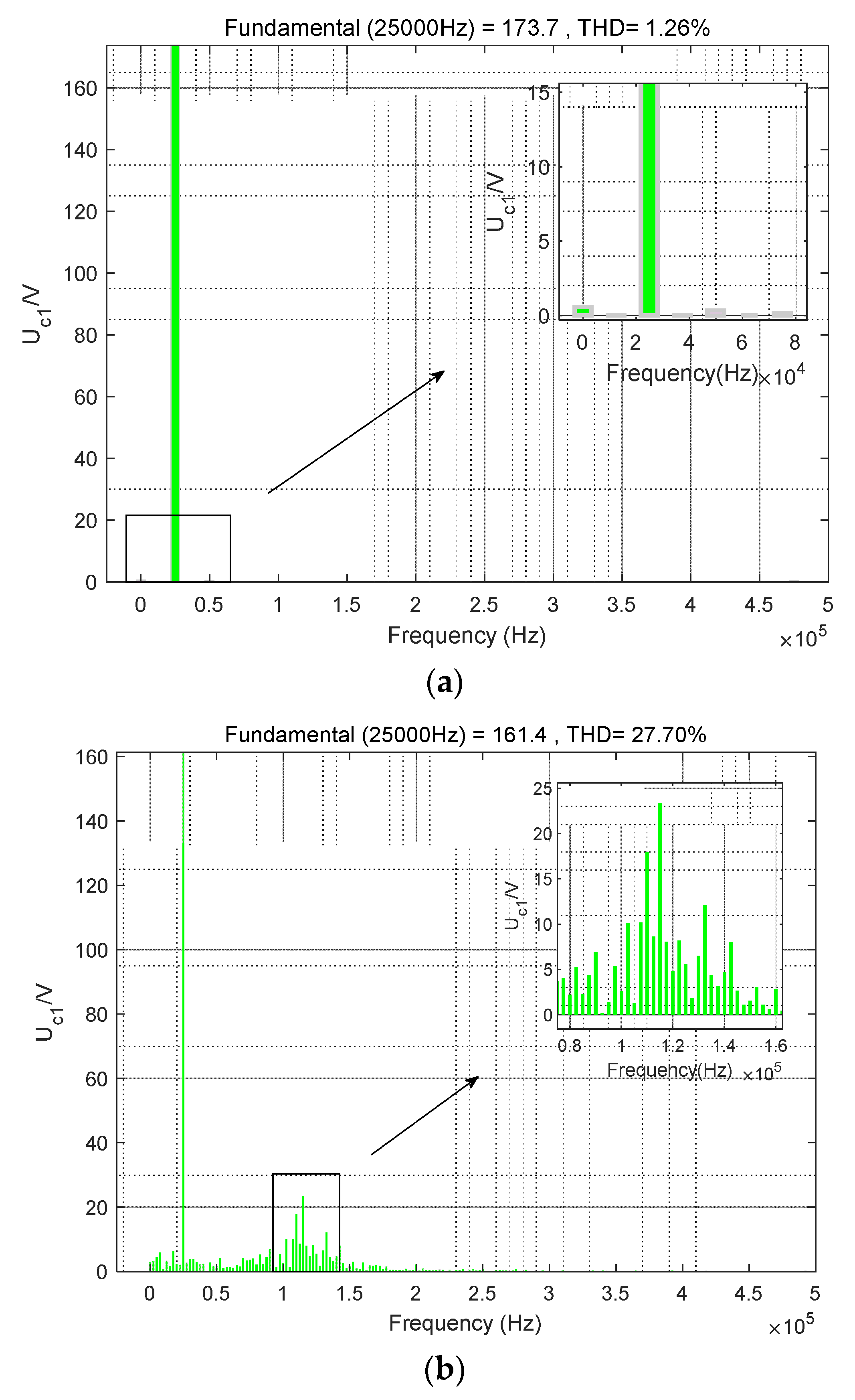
In addition, by importing the data into MATLAB and selecting a fundamental frequency of 25 kHz for spectrum analysis, the harmonic spectrum of voltage U_c1 can be obtained. As depicted in Figure 10a, it can be observed that when the resistance R is 5 KΩ, the total harmonic distortion (THD) of the output voltage U_c1 is measured at 1.21% within the frequency range of 0–500 kHz. Remarkably, the harmonics exhibit smaller amplitudes compared to the fundamental frequency, with each harmonic amplitude approximating 0 V. However, when the resistance R is 50 Ω, the THD of the output voltage U_c1 significantly increases to 27.70%. Under this condition, the system exhibits oscillations; the oscillation frequency is mainly around 110 KHz which is between the operating frequency of 25 kHz and the switching frequency of 500 kHz. This oscillation phenomenon can be called “low-frequency oscillation”. In the region of the oscillation frequency, the voltage U_c1 has larger harmonics. Therefore, the occurrence of low-frequency oscillation will make the fluorescent lamp work in harsh environments.

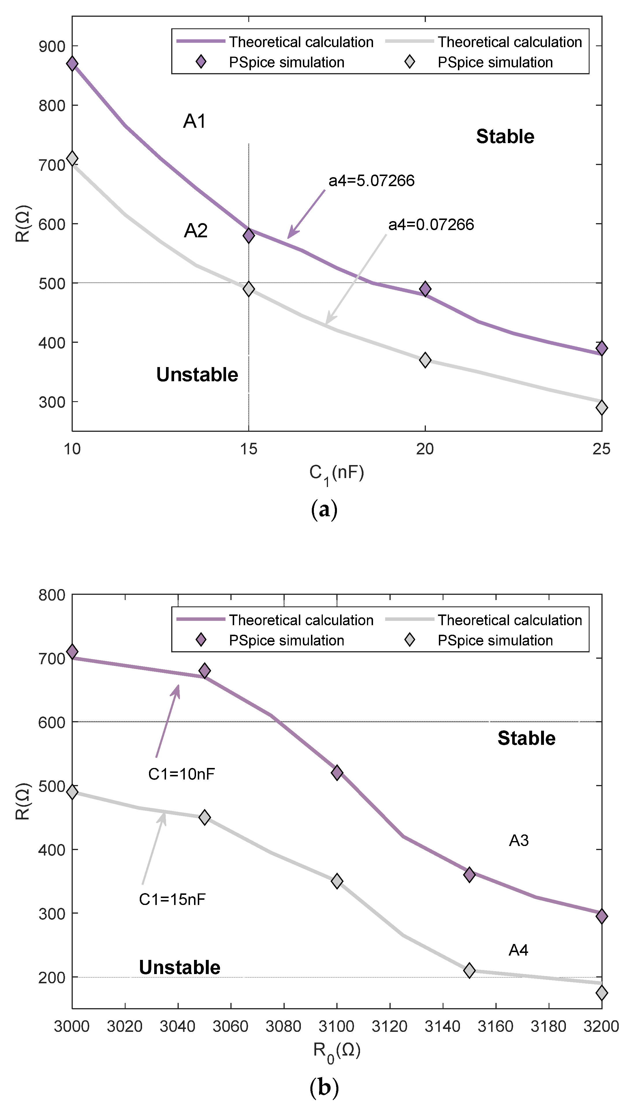
Figure 11a shows the stability boundary of the system obtained by PSpice simulations and theoretical calculations in the C₁-R parameter plane under different parameters a₄, indicating that with the decrease of capacitor C₁ or resistance R, the full-bridge inverter with the fluorescent lamp is more prone to instability. In addition, when a₄ = 0.07266, the stable region is A1 + A2, while when a₄ = 5.07266, the stable region decreases to region A1. Therefore, the stability region of the system will decrease with the increase of the parameter a₄. Figure 11b shows the stability boundary of the system obtained by PSpice simulations and theoretical calculations in the R₀-R parameter plane under different capacitance C₁, indicating that the full-bridge inverter with the fluorescent lamp is more prone to instability with the decrease of resistance R₀ or R. In Figure 11b, when C₁ = 15 nF, the stable region is A3 + A4, while when C₁ = 10 nF, the stable region is reduced to region A3. Thus, the stable region of the system will increase with the increase of the capacitance C₁. Based on the stability boundaries of the system, it is possible to optimize the parameter design of the system, thereby reducing the risk of system oscillation or even failure, and enhancing the reliability and stability of the system.

5. Conclusions

This paper presents the first analysis of the impact of fluorescent lamp memristive characteristics on the stability of a full-bridge inverter. It identifies the presence of low-frequency oscillations in a full-bridge inverter with a fluorescent lamp. By utilizing harmonic balance methods and Floquet theory, the essential mechanism generating low-frequency oscillations is unveiled as the occurrence of Hopf bifurcation in the system, along with establishing stability boundaries across different parameter planes. Additionally, PSpice models for both the fluorescent lamp and the entire system are developed, and the obtained simulation results are consistent with the theoretical analysis. Experiments will be conducted in future work. However, in general, under the premise of consistency between theoretical analysis results and PSpice simulation results, the theoretical analysis outcomes possess a higher level of reliability. The conclusion of this paper can offer guidance on parameters and control strategies for the design of a full-bridge inverter with a fluorescent lamp load. Moreover, it can facilitate the comprehension of instability mechanisms in systems incorporating memristive devices, thereby offering a foundation for the expansion of memristor applications.

References

1. Chua, L.O. Memristor-the missing circuit element. IEEE Trans. Circuit Theory 1971, 18, 507–519. [Google Scholar] [CrossRef]
2. Chua, L.O.; Kang, S.M. Memristive devices and systems. Proc. IEEE 1976, 64, 209–223. [Google Scholar] [CrossRef]
3. Chua, L.O. Everything you wish to know about memristors but are afraid to ask. Radioengineering 2015, 24, 319–368. [Google Scholar] [CrossRef]
4. Chua, L.O. If it’s pinched it’s a memristor. Semicond. Sci. Technol. 2014, 29, 104001. [Google Scholar] [CrossRef]
5. Strukov, D.B.; Snider, G.S.; Stewart, D.R.; Williams, R.S. The missing memristor found. Nature 2008, 453, 80–83. [Google Scholar] [CrossRef]
6. Ventra, M.D.; Pershin, Y.V.; Chua, L.O. Putting memory into circuit elements: Memristors, memcapacitors and meminduetors. Proc. IEEE 2009, 92, 1371–1372. [Google Scholar] [CrossRef]
7. Yin, Z.; Tian, H.; Chen, G.; Chua, L.O. What are Memristor, Memcapacitor, and Meminductor? IEEE Trans. Circuits Syst. II Express Briefs 2015, 62, 402–406. [Google Scholar]
8. Biolek, Z.; Biolek, D. How Can the Hysteresis Loop of the Ideal Memristor Be Pinched? IEEE Trans. Circuits Syst. II Express Briefs 2014, 61, 491–495. [Google Scholar] [CrossRef]
9. Biolkova, V.; Biolek, D.; Biolek, Z. Interpreting area of pinched memristor hysteresis loop. Electron. Lett. 2014, 50, 74–75. [Google Scholar]
10. Biolek, Z.; Biolek, D.; Biolkova, V. Computation of the Area of Memristor Pinched Hysteresis Loop. IEEE Trans. Circuits Syst. II Express Briefs 2012, 59, 607–611. [Google Scholar] [CrossRef]
11. Wang, L.C.; Yang, L.X.; Qin, K.J. Gas discharge lamp circuit characteristics. J. Electr. Technol. 1991, 3, 44–47. [Google Scholar]
12. Dai, G.J.; Gao, J.P. Dynamic PSpice Model of Fluorescent Lamp. China Light Light. 1999, 3, 2–5. [Google Scholar]
13. Yan, W.; Tam, E.; Hui, S.Y.R. A Semi-Theoretical Fluorescent Lamp Model for Time-Domain Transient and Steady-State Simulations. IEEE Trans. Power Electron. 2007, 6, 22. [Google Scholar]
14. Lin, D.; Hui, S.Y.R.; Chua, L.O. Gas Discharge Lamps Are Volatile Memristors. IEEE Trans. Circuits Syst. I Regul. Pap. 2014, 61, 2066–2073. [Google Scholar] [CrossRef]
15. Adhikari, S.P.; Sah, M.P.; Kim, H.; Chua, L.O. Three Fingerprints of Memristor. IEEE Trans. Circuits Syst. I Regul. Pap. 2013, 60, 3008–3021. [Google Scholar] [CrossRef]
16. Clauss, D.A.; Ralich, R.M.; Ramsier, R.D. Hysteresis in alightbulb: Connecting electricity and thermodynamics with simple experi-ments and simulations. Eur. J. Phys. 2001, 22, 385–394. [Google Scholar] [CrossRef]
17. Gandhi, G.; Aggarwal, V.; Chua, L.O. The detectors used in the first radios were memristors. In Memristor Networks; Springer International Publishing: Berlin/Heidelberg, Germany, 2014; pp. 53–66. [Google Scholar]
18. Corinto, F.; Ascoli, A. Memristive diode bridge with LCR filter. Electron. Lett. 2012, 48, 824–825. [Google Scholar] [CrossRef]
19. Robert, B.; Robert, C. Border collision bifurcations in a one-dimensional piecewise smooth map for a PWM current-programmed H-bridge inverter. Int. J. Control. 2002, 75, 1356–1367. [Google Scholar] [CrossRef]
20. Kousaka, T.; Sakamoto, K.; Ma, Y. Bifurcation and chaos in a PWM current-mode H-bridge inverter. In Proceedings of the National Conference on Nonlinear Systems & Dynamics, Chennai, India, 6–8 February 2006; pp. 1–4. [Google Scholar]
21. Wang, X.M.; Zhang, B.; Qiu, D.Y. The fast-and slow-scale stabilities and chaotic motion of H-bridge sine inverter. Acta Phys. Sin. 2009, 58, 2248–2254. [Google Scholar] [CrossRef]
22. Wang, X.M.; Zhang, B. Analysis of Bifurcation and Chaos in Single-phase SPWM Inverters. Trans. China Electrotech. Soc. 2009, 24, 101–107. [Google Scholar]
23. Wu, J.K.; Zhou, L.W.; Lu, W.G. Research on general bifurcated control strategy for Voltage Inverter. Acta Phys. Sin. 2012, 61, 210202. [Google Scholar]
24. Liu, H.C.; Li, F.; Su, Z.X.; Sun, L.S. Symmetrical dynamical characteristic of peak and valley current-modecontrolled single-phase H-bridge inverter. Chin. Phys. B 2013, 22, 110501. [Google Scholar] [CrossRef]
25. Zhang, H.; Dong, S.; Guan, W.; Liu, Y. Analysis of fast-scale bifurcation in peak current controlled buck-boost inverter based on unified averaged model. Int. J. Bifurc. Chaos 2016, 26, 1650074. [Google Scholar] [CrossRef]
26. Bao, B.; Zhang, X.; Bao, H.; Wu, P.; Wu, Z.; Chen, M. Dynamical effects of memristive load on peak current mode buck-boost switching converter. Chaos Solitons Fractals 2019, 122, 69–79. [Google Scholar] [CrossRef]
27. Zhang, J.P.; Yang, Y.; Wang, D.Q. Dynamic analysis and chaos control of the switched-inductor boost converter with the memristive load. Int. J. Circuit Theory Appl. 2021, 49, 2007–2020. [Google Scholar] [CrossRef]
28. Yang, Y.; Li, D.D.; Wang, D.Q. Dynamic analysis of the switched-inductor buck-boost converter based on the memristor. Electronics 2021, 10, 452. [Google Scholar] [CrossRef]
29. Zhang, R. High Performance Power Converter Systems for Nonlinear and Unbalanced Load/Source. Doctoral Dissertation, State University, Blacksburg, VA, USA, 1998. [Google Scholar]
30. Xu, G.J.; Huang, W.X. Research and Design of Electronic Ballast for Digital Fluorescent Lamp. J. Electron Devices 2011, 34, 202–205. [Google Scholar]
31. Kavehei, O.; Kim, Y.-S.; Iqbal, A.; Eshraghian, K.; Al-Sarawi, S.F.; Abbott, D. The fourth element: Insights into the memristor. In Proceedings of the 2009 International Conference on Communications, Circuits and Systems, Milpitas, CA, USA, 23–25 July 2009; pp. 921–927. [Google Scholar]
32. Yu, H.T.; Fang, X.B.; Jiang, Y.Z.; Li, X.X. Analysis of Capacitance and its parasitic parameters in Electromagnetic Compatibility Problems. Mech. Electr. Technol. 2019, 127, 66–70+89. [Google Scholar]
33. Pease, R. Analog Circuits: World Class Designs; Beihang University Press: Beijing, China, 2014; pp. 107–111. [Google Scholar]
34. Jiang, W.; Wu, R.H. A study on working stability of H-bridge inverter based on PI control. J. Vib. Shock. 2019, 39, 62–68. [Google Scholar]
35. Gong, R.X.; Yin, Z.H. A chaos control method of single-phase H-bridge photovoltaic inverter. Acta Phys. Sin. 2019, 70, 312–321. [Google Scholar] [CrossRef]
Figure 1. Comparison between the original formula and the result after fitting an approximation. (a) The fitting effect of a5T−0.75exp(ea6/(2kT)); (b) The fitting effect of a2exp(−ea3/(kT)).
Energies 16 06622 g001
Figure 2. Schematic diagram of a current feedback-controlled full-bridge inverter with fluorescent lamp load.
Energies 16 06622 g002
Figure 3. Simulation model for the system in the MATLAB/Simulink.
Energies 16 06622 g003
Figure 4. Simulation results in Matlab/Simulink under R = 5 kΩ (a) The voltage Uc1; (b) Current.
Energies 16 06622 g004
Figure 5. Simulation results in Matlab/Simulink under R = 50 Ω (a) The voltage Uc1; (b) Current.
Energies 16 06622 g005
Figure 6. Comparison between harmonic balance method and Simulink simulation.
Energies 16 06622 g006
Figure 7. Trajectory of Floquet multipliers λ1,2 and λ3 with R in the complex plane.
Energies 16 06622 g007
Figure 8. PSpice simulation of the system under R = 5 kΩ (a) Voltage Uc1; (b) Current.
Energies 16 06622 g008
Figure 9. PSpice simulation of the system under R = 50 Ω (a) Voltage Uc1; (b) Current.
Energies 16 06622 g009
Figure 10. Harmonic spectrum of Uc1 (a) R = 5 kΩ; (b) R = 50 Ω.
Energies 16 06622 g010
Figure 11. Under different parameters, the system stability boundary is compared by theoretical calculations and PSpice simulations (a) Different parameters a4 in the C1-R parameter plane; (b) Different parameters in C1 in the R0-R parameter plane.
Energies 16 06622 g011