PePTM: An Efficient and Accurate Personalized P2P Learning Algorithm for Home Thermal Modeling

Abstract

Nowadays, the integration of home automation systems with smart thermostats is a common trend, designed to enhance resident comfort and conserve energy. The introduction of smart thermostats that can run machine learning algorithms has opened the door for on-device training, enabling customized thermal experiences in homes. However, leveraging the flexibility offered by on-device learning has been hindered by the absence of a tailored learning scheme that allows for accurate on-device training of thermal models. Traditional centralized learning (CL) and federated learning (FL) schemes rely on a central server that controls the learning experience, compromising the home’s privacy and requiring significant energy to operate. To address these challenges, we propose PePTM, a personalized peer-to-peer thermal modeling algorithm that generates tailored thermal models for each home, offering a controlled learning experience with a minimal training energy footprint while preserving the home’s privacy, an aspect difficult to achieve in both CL and FL. PePTM consists of local and collaborative learning phases that enable each home to train its thermal model and collaboratively improve it with a set of similar homes in a peer-to-peer fashion. To showcase the effectiveness of PePTM, we use a year’s worth of data from US homes to train thermal models using the RNN time-series model and compare the data across three learning schemes: CL, FL, and PePTM, in terms of model performance and the training energy footprint. Our experimental results show that PePTM is significantly energy-efficient, requiring 695 and 40 times less training energy than CL and FL, respectively, while maintaining comparable performance. We believe that PePTM sets the stage for new avenues for on-device thermal model training, providing a personalized thermal experience with reduced energy consumption and enhanced privacy.

1. Introduction

1.1. Motivation

The intelligence of home automation systems has reached new levels thanks to the advanced sensing, communication, and control features of smart thermostats. In recent times, increasingly sophisticated smart thermostats have become commercially available [1,2,3,4]. With ample computational power to operate machine learning (ML) algorithms, conduct fine-tuning, and run a thermal model locally for control purposes, optimizing the local thermal environment has become achievable. Programmable thermostats cannot accomplish this task. Considerable research has been carried out to develop thermal models for homes. These models range from white-box models that comply with the laws of physics [5,6] to gray-box models that calculate the parameters of resistor–capacitance networks based on sensor data  [7,8,9,10] to black-box models that create time-series models dependent only on smart thermostat sensor data [11,12,13].

White- and gray-box models are usually very accurate in predicting heat dynamics. However, due to the peculiarities of each home, they cannot be easily developed. While there have been attempts to customize a generic model based on the characteristics of each home, access to metadata would be needed to carefully select the generic model that can be easily adapted to the target environment [7]. This has proven to be challenging “in the wild”. Black-box (i.e., ML or data-driven) models on the other hand have lower data needs and can be accurate enough for the target control application. In previous work, several types of models have been trained to predict changes in room temperature. These include (1) neural networks [12,13,14], such as recurrent neural networks (RNNs), and (2) time-series statistical models [11], such as ARMA, ARIMA, ARIMAX, and SARIMAX.

In this work, we use neural networks since they can be trained without in-depth knowledge of the home’s physical characteristics (such as its layout and construction materials), and can be potentially personalized and adapted to the local environment of each home. Since data emitted by sensors embedded in each smart thermostat may be biased and insufficient to fully train a neural network, our goal is to train these models on more diverse data, collected from several homes with similar characteristics.

1.2. Problem Statement

There are three main schemes for training a neural network, namely: centralized learning (CL), federated learning (FL), and peer-to-peer (P2P) learning. In centralized learning, we aggregate distributed data by sending them to a central server, where the model is trained. Since data collected by smart thermostats can contain private information (e.g., revealing the occupancy pattern of the home [15] or the household’s socioeconomic status [16]), clients need to trust the central server. In addition to privacy concerns, the central server is a single point of failure (SPoF), unless expensive and energy-intense replication mechanisms are properly implemented to ensure reliability. In FL, privacy concerns are addressed to some extent, as the central server aggregates model updates rather than raw data. However, the presence of an honest-but-curious server can potentially lead to the inference of private information from home updates (i.e., gradients). Furthermore, the aggregation server remains susceptible as a SPoF. A recently developed alternative involves peer-to-peer learning, in which the central server is eliminated [17,18]. This approach effectively mitigates the SPoF issue and mitigates privacy attacks, such as the attribute inference attack, which could be executed by an honest-but-curious server. In this scheme, each home independently trains its respective thermal model, and subsequently enhances the local model through collaboration with a set of similar homes.

1.3. Our Contributions

In this paper, we adopt the described P2P learning scheme and propose PePTM, a personalized peer-to-peer thermal modeling algorithm, which we implement on commodity devices, like mobile phones readily available at homes. PePTM allows training personalized thermal models without the need for a central server, ensuring the data privacy of homes. To investigate the advantages of PePTM over CL and FL, we use the data-driven RNN model to predict room temperature and explore how these models can be trained in an energy-efficient and accurate manner. In all experiments, it is assumed that the room temperature does not vary widely during a 15 min interval. To minimize the training time and, thus, the energy consumption of training the thermal models, we take advantage of two abstraction techniques: spatial abstraction through clustering in the case of FL and a sparse network of connected homes in the case of PePTM, and temporal abstraction through the downsampling of the thermostat’s sensor data. The empirical results demonstrate that, among the three learning schemes, and compared to the case where thermal models are trained traditionally (i.e., the abstraction techniques are not applied), the PePTM algorithm is extremely energy efficient, with 695 and 40 times less energy consumption than CL and FL, respectively. This can be attributed to the fact that the training of thermal models in PePTM is performed by inexpensive commodity mobile devices, without using a power-hungry central server, as in CL and FL. For performance comparison, we considered the root-mean-square error (RMSE) and mean absolute error (MAE), and found that the PePTM algorithm is comparable to CL and superior to FL with respect to both metrics. Thus, we corroborate that the PePTM algorithm trains thermal models with significantly less energy compared to the other two schemes, yet it still has better accuracy, without having to address the issues of SPoF and data privacy.

In this paper, we make the following contributions:

• We introduce PePTM, a peer-to-peer ML algorithm designed to efficiently train personalized home thermal models, without sharing data with a central server.
• We show that by connecting homes with a small set of similar neighbors, PePTM can learn accurate thermal models with minimal energy and network bandwidth.
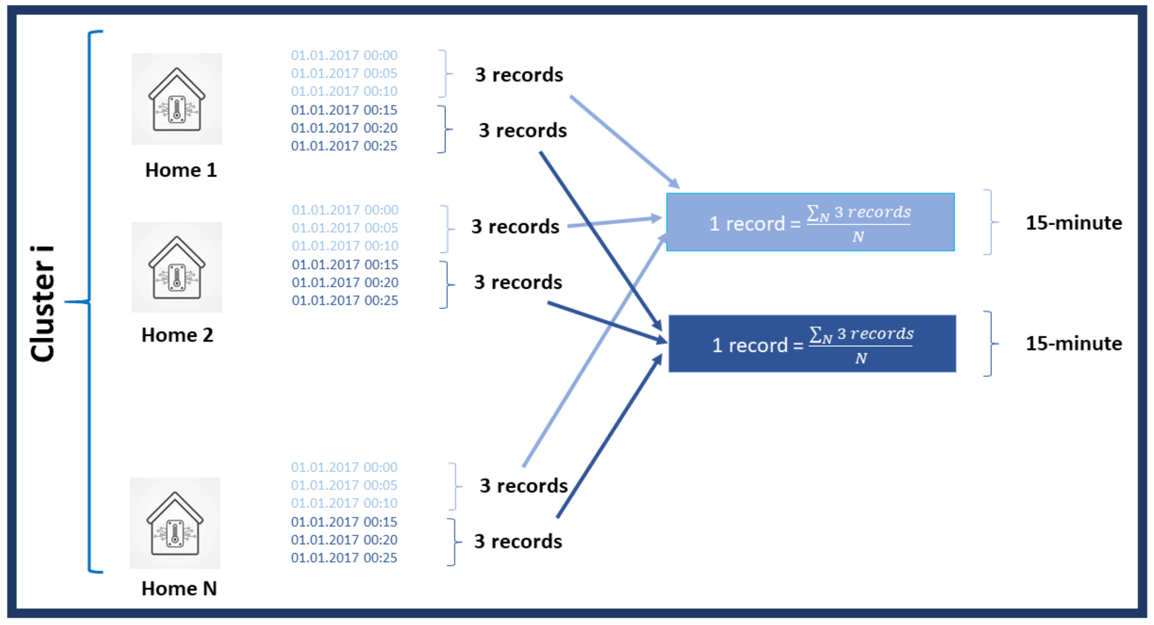
• To enable model training on mid-range mobile devices, we make use of temporal abstraction to reduce the size of sensor data, as well as spatial abstraction to minimize network bandwidth usage, allowing for efficient and personalized thermal models.
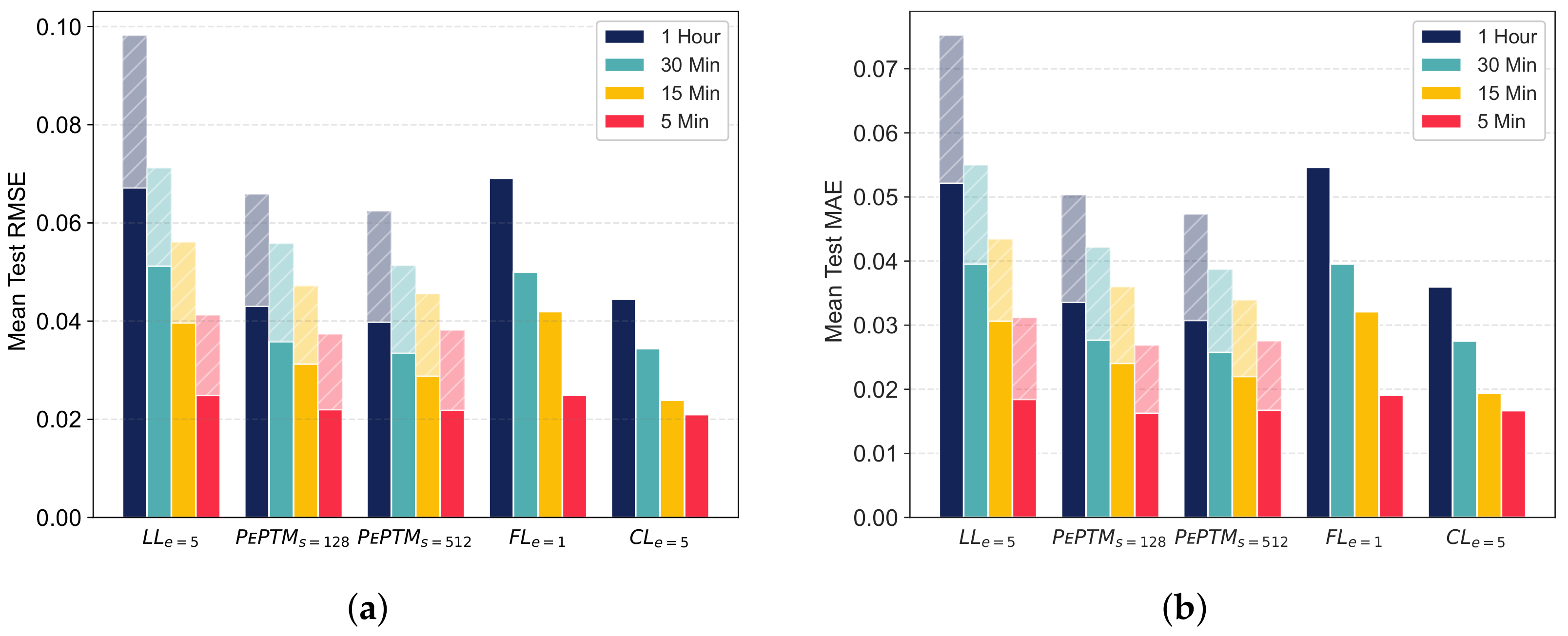
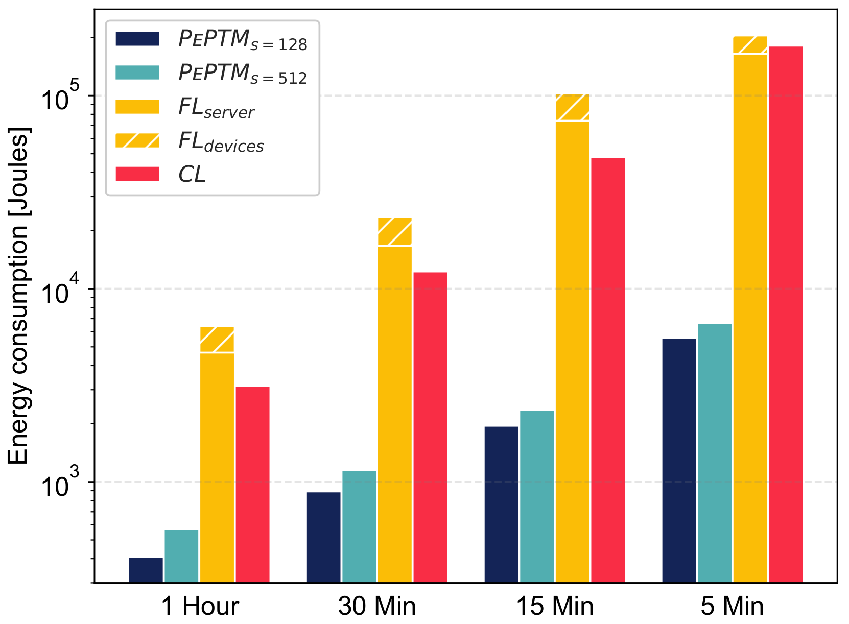
• We empirically evaluate the performance of PePTM under different abstraction scenarios, and we compare it with CL and FL, using RNN as the ML thermal model. Our experimental results show that PePTM is significantly energy-efficient, requiring 695 and 40 times less training energy than CL and FL, respectively, while still achieving at least comparable performance compared to CL and FL.

The rest of the paper is organized as follows. In Section 2, we provide an overview of previous related works. In Section 3, we outline the PePTM algorithm and its properties. In Section 4, we describe our methodologies, in terms of (1) spatial and temporal abstractions and (2) quantification of energy consumed by the three considered learning schemes. In Section 5, we compare the three learning schemes from the perspectives of energy and performance. In Section 6, we conclude and discuss future work.

2. Related Work

2.1. Thermal Models

Building operations accounted for 30% of global energy consumption and 27% of total energy sector emissions in 2021, according to the International Energy Agency (IEA) report [19]. The HVAC systems are responsible for up to 50% of the energy consumption of these buildings [20]. Thus, improving the energy efficiency of HVAC systems while maintaining thermal comfort for the occupants is critical to optimize the energy consumption of buildings and the global energy sector. To address this problem, many works have been suggested in the literature to model the thermal behavior of buildings and predict their temperature for optimal HVAC systems operation. These techniques can be classified into three categories, which will be presented next.

2.1.1. White-Box Models

This modeling approach is based on considering detailed information about the building, such as its geometry, structure, and thermal capacitance, to name a few, in order to generate complex mathematical models based on the laws of physics and thermodynamics  [6]. The white-box modeling approach is integrated with well-known simulation tools for building performance, like EnergyPlus [21]. While a well-calibrated white-box model can achieve high accuracy, it is often very difficult to obtain all the information required to establish such a model.

2.1.2. Black-Box Models

By leveraging data from the building’s smart thermostat, this approach constructs a predictive model for room temperature by utilizing various techniques, including time-series models, like the autoregressive (AR) model with exogenous input (ARX) [11], the autoregressive (AR) “moving-average” (MA) model with exogenous input (ARMAX) [22], and neural network models, like multilayer perceptron (MLP) [12,14] or long short-term memory (LSTM) [14].

2.1.3. Gray-Box Models

To carry out this modeling process, the building’s exterior and interior walls are divided into several temperature-consistent segments, which are then incorporated into a resistor–capacitance (RC) network [23]. The parameters of this model are then estimated using the data provided by the smart thermostat [7,8,24]. This identification problem can be computationally expensive for a high-order RC model. As a result, reduced-order RC models are sometimes preferred (e.g., 2R1C, 2R2C, or 3R3C), as they achieve a balance between accuracy and complexity [25].

2.2. Personalized Thermal Model Training

In this work, we consider multiple homes with the goal of training a thermal model, while taking into account their diverse climate zones and thermal properties. The use of white-box and grey-box models, based on the physical properties of buildings, can be challenging and may result in generic models that are not suitable for all homes. Therefore, we rely on the local sensor data provided by installed smart thermostats to learn black-box thermal models. We assume the availability of a limited number of accessible metadata, such as the location of the building, its floor area, and its approximate age.

Traditionally, sensor data are sent to a central server (the cloud) to learn a global thermal model that is supposed to be adequate for every home [26]. Such CL schemes raise many privacy and security concerns, given the sensitive nature of the sensor data [15]. Another aspect of CL is the significant energy consumption dedicated to collecting and training the thermal model on the cloud, which may go against the whole purpose of saving energy in the first place. Furthermore, learning a global thermal model may not satisfy the thermal requirements of most home occupants. To alleviate some of these concerns, FL [27] emerged as a solution to enable the training of ML models using distributed data. Here, data are not shared with the server, and homes engage in model training locally, under the coordination of the server. However, FL still suffers from some of the aforementioned drawbacks: the server is always consuming energy, and the output is a generic thermal model. Moreover, the server is a potential SPoF in both CL and FL.

In this paper, we consider a completely decentralized setting, where each home has its own local thermal model and personalized learning objectives, which it seeks to improve by communicating with other homes within a peer-to-peer network. Many similar approaches have been presented [17,18,28,29] to train personalized ML models. Ref. [17] used the alternative direction method of multipliers (ADMM). Ref. [18] proposed a robust algorithm to fight against malicious peers, and generalized it to support dynamic networks, where peers can change their neighbors if they are malicious or have no beneficial information. Ref. [28] tackled the privacy issue by proposing a differentially private algorithm, which enables peers to efficiently learn personalized models under strong privacy requirements. To learn personalized models, the authors in [29] suggested jointly learning the network graph with the models to achieve lower communication costs. Recently, ref. [30] introduced the P3 algorithm to allow peers connected to a peer-to-peer network to efficiently train ML models (using their smartphone devices only).

In this paper, we adopt the peer-to-peer learning scheme and propose the new PePTM algorithm to enable homes with varying amounts of sensor data and computational abilities to train their personalized thermal models in an energy-efficient manner. To the best of our knowledge, we are the first to provide a peer-to-peer solution for home thermal modeling and propose a methodology for training personalized thermal models.

3. Personalized P2P Learning of Home Thermal Models

Our goal is to develop a machine learning-based thermal model using data from smart thermostat sensors in a set of homes. The model will take into account the thermal models of other similar homes within a peer-to-peer network graph, which represents a semantic overlay. This allows for the privacy and anonymity of home identities and private data. Each home aims to personalize its thermal model while incorporating knowledge from similar homes to improve its model in a privacy-preserving manner. Throughout this paper, the term “home” refers to both the physical residence and the communication device used for training the model.

3.1. Formal Definition

We consider a set of n homes organized in a weighted, undirected graph $G=(V,E)$. The vertex set V of size n represents homes, and E denotes the set of weighted edges between homes. The weight values reflect a notion of similarity between each pair of homes, represented by a symmetric non-negative similarity matrix $W\in {\mathbb{R}}^{n\times n}$, as suggested by [17,18]. Given two homes, i and j, $W_{ij}$ is the weight of edge $(i,j)\in E$, representing the level of similarity between i and j. $W_{ij}$ tends to be large (resp. small) if i and j have similar (resp. dissimilar) characteristics. Furthermore, if i is not linked to j, the similarity is equal to zero (i.e., $W_{ij}=0$). We set $W_{ij}=0$ if $i=j$, $D_{ii}={\sum }_{j=1}^n{W}_{ij}$, and denote by ${\mathcal{N}}_i=\{j:W_{ij}>0\}$ the set of neighbors of home i. We assume each home i has access to its neighbors’ associated weights without having a global view of the network.

Each home i holds a local dataset $S_i={\{x_i^j,y_i^j\}}_{j=1}^{m_i}$ consisting of $m_i=\left|S_i\right|$ training samples derived from smart thermostat sensor data, independently drawn from the data distribution of the personalized machine learning problem of home i. We consider a feature space ${\mathcal{X}}_i$ and a label space ${\mathcal{Y}}_i$ defining a personalized supervised learning task, with an unknown probability distribution $P({\mathcal{X}}_i,{\mathcal{Y}}_i)$, and a loss function l. Ideally, each home would like to minimize the expected risk given by:

$$R\left(w\right)=\underset{\mathcal{X}\times \mathcal{Y}}{\int }l(w,x^j,y^j)dP(x^j,y^j).$$

(1)

Since $P(x,y)$ is unknown, the empirical risk is usually used as an unbiased estimate of the expected risk. It is simply the average number of losses over the home’s local data:

$$R_{m_i}\left(w\right)=\frac{1}{m_i}\sum _{j=1}^{m_i}l(w,x^j,y^j)$$

Intuitively, a home can train its thermal model locally using only its thermostat sensor data, without any communication. However, relying solely on local data can result in learning models that are either weak due to a lack of sufficient training data (e.g., new homes or homes with newly installed smart thermostats), or do not generalize well if the available data are not representative of the overall distribution. Furthermore, homes may have limited processing capabilities (e.g., IoT devices or mobile devices) and may be unwilling to share their raw data, due to privacy or communication constraints. Our objective is to enable collaboration between homes within the peer-to-peer network graph G, where homes can enhance their locally trained models with the help of other homes while maintaining accurate and personalized models with respect to their local data.

To ensure full control over the peer-to-peer learning process, we define the cost function for each home that participates in training as follows:

$$F_i\left(w\right)=\mu R_{m_i}\left(w\right)+(1-\mu )\frac{1}{\left|{\mathcal{N}}_i\right|}\sum _{j\in {\mathcal{N}}_i}\left(W_{ij}{R}_{m_j}\left(w\right)\right)$$

(2)

where $\mu \in [0,1]$ is a personalization parameter to control the effect of the network updates over the locally computed updates. Large values of $\mu$ prevent the model from diverging too much from the local data, while small values enable greater network influence. Notice that Equation (2) encompasses two extreme cases: when $\mu \to 1$, homes learn purely local models, and when $\mu \to 0$, homes learn a global model.

3.2. PePTM Algorithm

This section presents PePTM (see Algorithm 1), a personalized peer-to-peer algorithm that enables homes with different thermal properties to learn personalized and accurate thermal models. PePTM is a collaborative learning algorithm designed to solve the personalized training problem in Equation (2). Homes in PePTM communicate in a semi-asynchronous fashion to exchange updates with their neighbors, without having a global view of the network. The communication is either established through direct TCP connections between homes or via a publish–subscribe pattern via the GossipSub protocol [31]. In scenarios with a stable and sparse network graph (minimal churn and low degree), TCP connections are suitable and easier to implement for update exchange. In contrast, in dense networks with frequent connect–disconnect cycles (i.e., churn), a publish–subscribe pattern offers a more efficient communication mechanism among neighboring homes. It is important to note that PePTM does not wait for all messages to be received before performing updates, enabling homes to continue updating their models if a neighbor disconnects or even if no messages are received. Finally, we assume that each peer becomes active when its local clock ticks following a Poisson distribution.

PePTM consists of two phases: a local learning phase, where each home learns a thermal model $w_i^{loc}$ locally, and a collaboration phase, where peers collaborate to enhance their locally trained models. We assume that all thermal models are initialized using a random weight vector with a controlled seed.

3.2.1. Local Training Phase

During local training, homes train an initial thermal model $w_i^0$ representative of their local data. We assume that local training is performed for a small number of epochs (typically, one or two epochs) due to the limited computing power of most homes, which usually use already available commodity devices (such as IoT or mobile devices) for training. Once an initial thermal model is obtained, indicating that the home’s thermal behavior is reasonably captured, transitioning to the collaborative phase is considered. This is because multiple local training epochs can become computationally expensive or infeasible with large local datasets and may lead to overfitting, preventing homes with low-quality data from generalizing their models. Joining the collaborative phase after a few local epochs ensures both computational efficiency and model effectiveness.

3.2.2. Collaborative Training Phase

Once a home i completes its local training phase, it can start collaborating with its neighbors to improve its local model and compensate for the lack of data or its limited computing power. At each timestamp t, a home i wakes up and performs the following steps consecutively:

• Communication step: Home i samples a mini-batch of size $s_i$ from its local dataset $S_i$ and uses it to calculate the gradient vector $v_i^t$, which is then broadcast to its set of neighbors ${\mathcal{N}}_i$.
• Update step: Upon receiving enough gradients, each home i evaluates the received gradients using a filtering component that computes ${\parallel v_i^t-v_j^t\parallel }^2$, and only accepts the ones that yield a norm difference below a given threshold, ${\sigma }_i$. The accepted gradients are then aggregated using weighted averaging to calculate the collaborative update $v_{\ast }$ as follows:

  $$v_{\ast }=\frac{1}{\left|accepted\right|}\sum _{j\in accepted}\frac{W_{ij}}{D_{ii}}{v}_j$$

  (3)
  The next model update $t+1$ is derived from a combination of the local update v and the collaborative update $v_{\ast }^t$, which can be controlled using the personalization parameter ${\mu }_i$ as follows:

  $$v\leftarrow {\mu }_i{v}_i^t+(1-{\mu }_i)v_{\ast }$$

  (4)

Following these two steps, PePTM allows homes with varying computational capabilities to participate in the collaborative phase of model training by using adequate sample sizes $s_i$. Thus, it democratizes the participation in ML training of thermal models for all homes. To further enhance collaboration, the weighted averaging aggregation rule defined in Equation (3) enables weighted updates based on the similarity between each neighboring home, enabling a faster convergence rate.

Algorithm 1 The PePTM Algorithm

Input: Network graph G; similarity matrix W; aggregation rule $\mathbb{A}$; learning rate $\gamma$.

Output: Personalized model with weights $w_i$ for every home $i\in G$.

1: upon event $<p2p.Init>$ do 2:       for each home $i\in G$ do 3:             $w_i^0\leftarrow$ locally trained model $w_i^{loc}$ 4:             broadcastGrads(0); 5: end event 6: procedure $broadcastGrads$ (t)         ▹ Trigger collaboration at epoch $t\in \left[T\right]$ 7:       ${\mathcal{D}}_i\leftarrow$ Draw $s_i$ samples without replacement from $S_i$; 8:       $v_i^t=\nabla \ell (w_i^t;{\mathcal{D}}_i)$ 9:       $\mathbf{trigger}<p2p.Broadcast|neighbors,[v_i^t]>;$ 10: upon event $<p2p.Receive|neighbor,[v_j^t]>$ do 11:       $V^t\leftarrow V^t\cup \left\{v_j^t\right\}$ 12:       if enough gradients are received for epoch t then 13:           collaborativeUpdate($V^t$); 14:           broadcastGrads($t+1$); 15: end event 16: procedure $collaborativeUpdate$ ($V^t$) 17:       for each gradient $v_j^t\in V^t$ do 18:           if ${∥v_i^t-v_j^t∥}^2<{\sigma }_i$ then 19:              $accepted\leftarrow accepted\cup \left\{\overline{v_j^t}\right\}$ 20:       $v_{\ast }^t=\frac{1}{\left|accepted\right|}\sum _{j\in accepted}\frac{W_{ij}}{D_{ii}}{v}_j$          ▹ With $D_{ii}={\sum }_{j=1}^n{W}_{ij}$ 21:       $v^t\leftarrow {\mu }_i{v}_i^t+(1-{\mu }_i)v_{\ast }$            ▹${\mu }_i$ is a personalization parameter 22:       $w_i^{t+1}\leftarrow w_i^t-\gamma v^t$

3.3. Properties of PePTM

Our goal is to enable different kinds of homes to join the network to learn accurate and personalized thermal models, regardless of their computational capabilities or the amount of data they possess. PePTM has the following three properties to support this goal:

3.3.1. Flexibility

A given home can train its model on several data samples $s_i$, depending on the available computational power it has. Homes with sufficient computational power can train on large data samples per round, while homes with computational- and energy-constrained devices (e.g., IoT devices) can train their models on a few samples per round. The flexibility of PePTM allows weak devices to transmit their updates within a reasonable time frame, thereby ensuring their gradients are considered during the update phase.

3.3.2. Confidence

Although we consider a setting involving only honest homes, our filtering component can mitigate simple attacks, such as crash failures and updates containing random or extreme values. This is achieved by discarding vectors that significantly deviate from the estimated gradient of the home. Homes with higher confidence in their data can set ${\sigma }_i$ to a small value to reduce the effect of network updates.

3.3.3. Personalization

To achieve a personalized thermal model, homes that possess a substantial amount of historical sensor data can set their personalization parameter ${\mu }_i$ to a high value (e.g., $\mu =0.9$), preventing their thermal model from diverging too far from the knowledge embedded in their local data and can result in faster convergence. Meanwhile, new homes or homes that have recently installed smart thermostats may want to opt for smaller values of ${\mu }_i$ (e.g., $\mu =0.5$) to allow for greater contribution from the network graph (i.e., neighboring peers) and improve the performance of the learned thermal model. The parameter ${\mu }_i$ creates a balance between optimizing the accuracy of the thermal model and preserving personalization. The choice of ${\mu }_i$ is determined by a multitude of factors, such as data availability and quality, and is tailored to the specific circumstances of each home. It is worth noting that ${\mu }_i$ can be adjusted dynamically as more data become available, allowing for continuous refinement of the thermal model.

4. Methodology

We present our methodology for efficient training of thermal models using the three described learning schemes: CL, FL, and P2P (i.e., our PePTM approach). We explain how we evaluate the performance and energy use of these models, and how we perform client selection in the distributed setting to allow similar homes to perform collaborative model training.

4.1. Temporal Abstraction

Smart thermostats typically feature multiple sensors that continuously monitor both indoor and outdoor temperatures at high frequencies, usually every five minutes, for real-time tracking. However, since indoor temperature fluctuations over such short intervals are minimal, it may be unnecessary to include them in temperature prediction models. Therefore, we propose using numerical abstraction techniques [32] to approximate larger time intervals of the home’s environment. This approach helps to reduce the data size for more efficient training and energy-saving during model development. Additionally, this method allows homes to share sensor data more securely by downsampling to 15 min, 30 min, or one-hour intervals. Figure 1 provides a visual depiction of the 15 min time interval abstraction method, where the records of N homes of a given cluster i and for 15 min intervals are replaced by one record representing the corresponding average.

4.2. Peculiarities of Homes

Buildings possess distinct thermal characteristics influenced by factors, such as location, floor area, and age. Consequently, the concept of training a global thermal model to encapsulate the thermal properties of all homes is not a realistic solution. To tackle this challenge, we suggest allowing similar homes to train individual thermal models collaboratively. Hossain et al. [7] demonstrated that homes situated in the same climate zone and featuring comparable floor area and age manifest similar thermal behaviors. Inspired by this, we designed two home selection strategies as described below.

Figure 1. The proposed temporal abstraction is visually represented through the utilization of 15 min time intervals. Comparable homes are assembled into cluster i, composed of N homes. The data collected from these homes are condensed and downsampled on the server for CL, while for FL and PePTM, downsampling occurs on the device.

Figure 1. The proposed temporal abstraction is visually represented through the utilization of 15 min time intervals. Comparable homes are assembled into cluster i, composed of N homes. The data collected from these homes are condensed and downsampled on the server for CL, while for FL and PePTM, downsampling occurs on the device.

4.2.1. Clustering

Homes with similar characteristics naturally exhibit analogous thermal behaviors, creating an opportunity for collective thermal model training. For instance, homes possessing comparable floor areas often install HVAC systems of the same capacity. Additionally, when comparing new homes constructed with thermal insulation to older homes that typically lack adequate insulation, the requirement for larger HVAC systems becomes apparent. In our approach, we harness these factors to cluster homes. We leverage fundamental home attributes, such as location, floor area, and age, to perform clustering on normalized values of “floor area” and “age” using the k-means algorithm. The objective was to group similar homes together in a few clusters, with the optimal number of clusters k determined using the elbow method [33].

Homes within a cluster can either send their data to the cloud (i.e., CL) or collectively train a representative model using FL, under the coordination of a central server. Alternatively, homes within the same cluster can collaboratively learn personalized models by directly connecting to each other in a peer-to-peer fashion, without relying on a central server using our PePTM algorithm.

4.2.2. Similarity Matrix

In the peer-to-peer setting, connecting each home with the rest of the cluster may require considerable network bandwidth, to maintain active connection and exchange model updates. Additionally, even within a cluster, updates from different homes should not be considered similar, as some homes are more similar than others. To overcome these issues, we propose building a similarity matrix W, formally defined in Section 3.1, where similar homes are connected through weighted edges that reflect the degree of similarity between a home and its neighbors. To derive the pairwise similarity between homes, we use the normalized Euclidean distance on the same basic floor area and age properties used in our clustering strategy, as follows:

$$d_{ij}=Norm\left[\sqrt{{(u_i-u_j)}^2+{(v_i-v_j)}^2}\right]$$

$$W_{ij}=\left\{\begin{array}{cc}1-d_{ij},\hfill & \mathrm{if}{d}_{ij}\le \rho \hfill \\ 0,\hfill & \mathrm{otherwise}\hfill \end{array}\right.$$

(5)

where $d_{ij}$ is the normalized Euclidean distance, and $u_i$ and $v_i$ are the floor area and the age of the home i, respectively. $\rho$ is the network density parameter to control the average number of neighbors a home can have. Using smaller values of $\rho$ results in a sparse network graph, where homes have fewer neighbors; using larger values of $\rho$ leads to a denser network graph, where homes have more neighbors.

4.3. Energy Analysis

The thermal requirements of homes vary with seasons, and require regularly updating the thermal behaviors of HVAC systems [34]. Most state-of-the-art approaches [7,34] ignore the non-negligible energy footprint of regularly training these thermal models. Here, we describe our approach for analyzing the energy required to train such models, under the three ML schemes we consider in this paper.

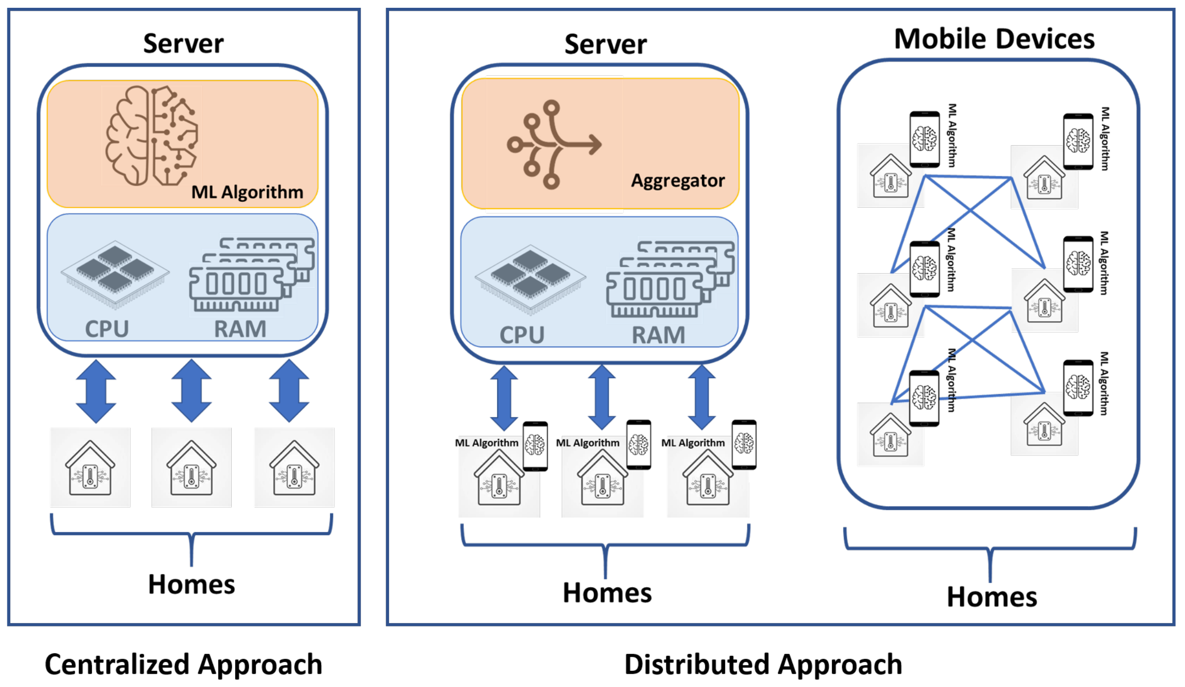
4.3.1. Centralized Approach

This energy analysis approach is related to the experiments conducted under the CL scheme. Here, a central server is responsible for collecting data from different homes to train a global thermal model. To measure the energy consumed by the server during the training, we consider the methodology described in [30] to compute the energy consumption of the ML model training: (1) one core of the processor is shielded, so that neither the operating system routines nor any other processes (i.e., applications) run on this specific core; (2) the corresponding ML algorithm is pinned to the shielded core; (3) the power profiler (i.e., kernel-based governors, such as on-demand, performance, or user space) is configured so that the underlying frequency of the core is fixed; (4) we use the powerstat tool to record key performance indicators (KPI), e.g., execution time, average power demand.

To calculate the dynamic power demanded by the underlying ML algorithm, we first kept the corresponding server idle (i.e., only the necessary operating system routines were running) for a duration of 10 min, where the average power demand was computed. Then, the dynamic power demand of the algorithm is derived by subtracting the overall demand from the idle power demand. Once the average dynamic power demand of the ML algorithm is computed, it is used to calculate the overall energy consumption by multiplying the average power demand by the execution time of the ML algorithm.

4.3.2. Distributed Approach

This energy analysis approach is related to the experiments conducted under the FL and PePTM schemes. For FL, a central server is responsible for coordinating the training process of the model, jointly trained by the participating homes. For each round, homes send the locally updated model to the central server, which performs model aggregation, and sends back the updated model. In this setup, the central server is the same as the one introduced in Section 4.3.1, and we adopt the same methodology to measure its energy consumption. Additionally, we implemented a custom sleeping mechanism, to reduce unnecessary waste of energy. To this end, the server goes into the deepest sleep mode, until the internet interfaces receive wake-up calls from homes, and start aggregating the received thermal models. Then, the server sends back the updated model to all homes. Note that the process of aggregating the received thermal models is not computationally intensive, which can be efficiently achieved by using the CPU. Consequently, no GPUs were used for the experiments in this approach, where the training of the individual model is performed by homes running on mid-range Android devices. For the PePTM setting, no central server is involved, and the training of each model is conducted collaboratively, with neighboring homes using mid-range Android devices.

To compute the energy use of training ML thermal models on mobile devices, we use the Power Profiler [35] to collect (at specific intervals) key performance indicators (e.g., current, voltage, execution time). From the collected information, power demand is derived by multiplying current by voltage, and this demand is multiplied by the execution time to compute the overall energy of the monitored application (i.e., the PePTM algorithm). The total energy consumption of the corresponding ML algorithms is derived by multiplying the number of homes by the energy consumption of each home. It is worth mentioning that the energy consumption of communication, either between homes (PePTM) or between homes and the central server (CL and FL) is out of the scope of this paper, and is therefore not considered in our approaches.

Figure 2 presents a graphical demonstration of the above-mentioned centralized and distributed approaches. Note that, for the distributed case, FL and PePTM schemes operate differently, such that the homes’ model training in both schemes is implemented by means of energy-efficient mobile devices. Furthermore, in addition to the architectural differences, the major dissimilarity between centralized and distributed approaches is the amount of information exchanged between the workers and the server. In the centralized case, homes need to send their local data to the central server, while in the case of the decentralized approach, homes only send their local model updates (no data exchange is involved) to the central server (for FL) or their neighboring peers (for PePTM).

4.4. ML Models’ Performance Evaluation

In this paper, we considered two performance metrics to assess the accuracy of the predictions ${\widehat{T}}_k$ generated by the ML thermal models with respect to the real observed values $T_k$: root mean squared error (RMSE) and mean absolute error (MAE). Note that neither the mean absolute percentage error (MAPE) nor mean percentage error (MPE) metrics [36] were considered because those two metrics are inappropriate for a normalized dataset, which was the case for our experiments.

4.4.1. Root Mean Square Error

RMSE is the standard deviation of the distance between the predicted and real observed values, and is given by:

$$RMSE=\sqrt{\frac{1}{n}\sum _{t=1}^n{|T_k-\widehat{T_k}|}^2}$$

(6)

Since it is the square root of the mean square error (MSE), this metric (like MSE) is highly affected by large errors [37]. This is because they are squared before taking the average.

4.4.2. Mean Absolute Error

MAE is the average of the distance between the predicted and observed values, and is given by [38]:

$$MAE=\frac{1}{n}\sum _{t=1}^n|T_k-\widehat{T_k}|$$

(7)

For each observation, the distance between the predicted and observed values is added. Then, the sum of the differences is divided by the number of observations, to obtain the average per observation.

5. Evaluation

In this section, we first introduce the dataset and the configured temporal abstraction scenarios used in our experiments. Next, we present an exhaustive set of experiments to highlight the practical advantages of our thermal model training methodology in terms of convergence rate and energy efficiency. We evaluate the PePTM algorithm under several configurations and compare it to FL and CL. Finally, we demonstrate the flexibility of PePTM, allowing all kinds of homes to participate in personalized thermal model training, regardless of their data or computational resources.

5.1. Experimental Setup

5.1.1. Implementation Details

Hardware: In our experiments, we used two hardware configurations to evaluate our approach: a powerful Linux-based server workstation, simulating the central server, akin to those commonly provided by cloud service providers for both CL and FL; and a set of mid-range Android mobile devices, representing resource-constrained devices (i.e., those with limited computing power and energy supply) commonly found in households. We chose the latter configuration to demonstrate that our proposed algorithm can effectively operate on readily available commodity devices in households, without the need for powerful, specialized machines to participate in the collaborative training process. The hardware and software specifications of both configurations are outlined in

Table 1. Hardware and software characteristics of the server workstation and Android devices used in the experiments.

Platform	OS	CPU	Frequency	RAM
Linux Server	Ubuntu 20.04 LTS	Intel Xeon W-2123	Min 1.2 GHz Max 3.6 GHz	32GB DDR4
Android Device	Android 11	Qualcomm SDM710	Min 1.7 GHz Max 2.2 GHz	4GB DDR4

. All experiments involving the server were performed using the middle-frequency value of the processor (i.e., 1.7 GHz), which yields the most energy-efficient training results compared to the highest and lowest CPU frequencies.

Source code: Our implementation of the three schemes can be accessed at https://github.com/karimboubouh/Thermal-PEPTM (accessed on 7 August 2023) for both Linux workstations and Android mobile devices. The source code was written in Python 3.10. For the server, the ML models were constructed using TensorFlow 2.9.1, while for Android, the models were written from scratch using NumPy 1.23.3 and packaged using Kivy 2.1.0. To measure the energy consumption of the algorithms on Android, we used the Power Profiler [35]. Its source code can be found at https://github.com/karimboubouh/PowerProfiler (accessed on 7 August 2023).

5.1.2. Smart Thermostat Dataset

To evaluate the proposed approaches, we use the smart thermostat Ecobee dataset [39] collected within the context of the “Donate Your Data” initiative. The dataset comprises data from 1000 homes distributed across four states in the US, namely California, New York, Texas, and Illinois. It consists of time-series data with a 5 min resolution collected over a period of 12 months in 2017, covering all four seasons. Additionally, the dataset includes metadata related to the homes where the thermostats are installed. The total size of the dataset is 34 GB, and it encompasses the following features: “Floor area” (Square foot), “Age” (Scalar, year of construction), “Indoor temperature” (Fahrenheit), “Outdoor temperature” (Fahrenheit), “Indoor humidity” (%RH), “Outdoor humidity” (%RH), “Indoor cool setpoint” (Fahrenheit), “Indoor heat setpoint” (Fahrenheit), and “Operating mode of HVAC” (Boolean).

5.1.3. Temporal Abstraction Scenarios

In our experiments, we established four distinct scenarios to train thermal models under three learning schemes (CL, FL, and PePTM), employing the widely-used RNN time-series ML model. In the first three temporal abstraction scenarios, namely “1 Hour”, “30 Min”, and “15 Min”, the data records of homes within the same time interval (i.e., 15, 30, or 60 min) are averaged to a single record for each timestamp. Subsequently, the resolution of the resulting records is reduced to the specified time interval. This downsampling technique substantially reduces the size of the training dataset, thereby enabling even weak devices to participate in the training, while simultaneously saving network bandwidth during the transmission of raw data in the case of CL. The fourth scenario corresponds to the 5 min interval, where we only average the data records in CL, without data downsampling. Figure 1 shows an example of using the “15 Min” scenario. For the case of CL only, we consider a fifth scenario and call it “RAW”, referring to the traditional way of sharing raw data with the server in CL, without any abstraction.

5.1.4. Network Settings

To group homes into fully connected clusters, we applied k-means using the age and floor area properties of the 1000 homes. This resulted in the creation of 6 clusters of approximately 200 similar homes, except for one cluster grouping a limited number of homes with large floor areas (e.g., hospitals) or very old buildings. To achieve a sparse network graph instead of fully connected clusters in PePTM, we used the concept of the similarity matrix described in Section 4.2.2. To determine the optimal value for the network density parameter $\rho$, a set of experiments was conducted by considering the density values of $0.01$, $0.05$, $0.3$, $0.6$, and $0.9$, which represent an estimated percentage of the total number of homes to be considered as neighbors for each home.

5.1.5. Used Parameters for Training

In order to assess our method of training models, we examined the state-of-the-art RNN time-series ML model. For the thermal model training, we utilized 85% of the data, while the remaining 15% was reserved for testing. Specifically, we allocated two and a half months of data from each season (i.e., 3 months) for training, and the remaining 15 days were dedicated to assessing (i.e., testing) the models produced. Unless specified otherwise, all experiments were conducted on cluster 0 during the summer season of 2017, considering the 207 homes within this cluster. The thermal model was trained for 5 epochs ($e=5$) during the experiments conducted under the CL setup (note: the 207 homes sent their data to the server, and then the server trained the thermal model for 5 epochs using the received data from all homes). For the FL setup, we trained a global thermal model for 100 rounds, with each home locally training the received thermal model for a full epoch ($e=1$) before sending back the new model to the server for aggregation. For PePTM, each home locally trained an initial model for one single epoch ($e=1$) using its local data. Next, the homes join the collaborative training phase; for each round, they train their personalized thermal models on a small number of samples s. These samples were configured with batch sizes s of 128 (the default value), $256,512$, and 1024 samples for each round. PePTM was executed using different numbers of rounds: 1, 50, 100, …, 450, and 500.

5.2. Experimental Results

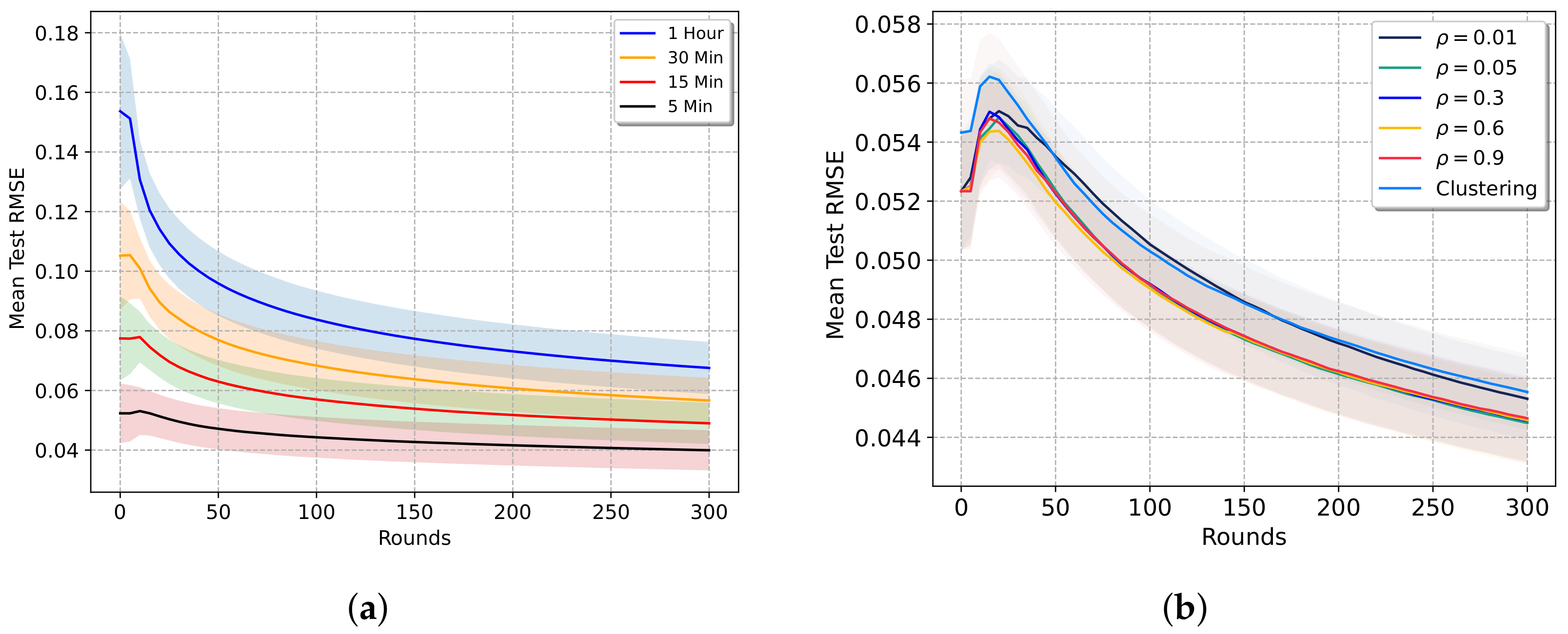
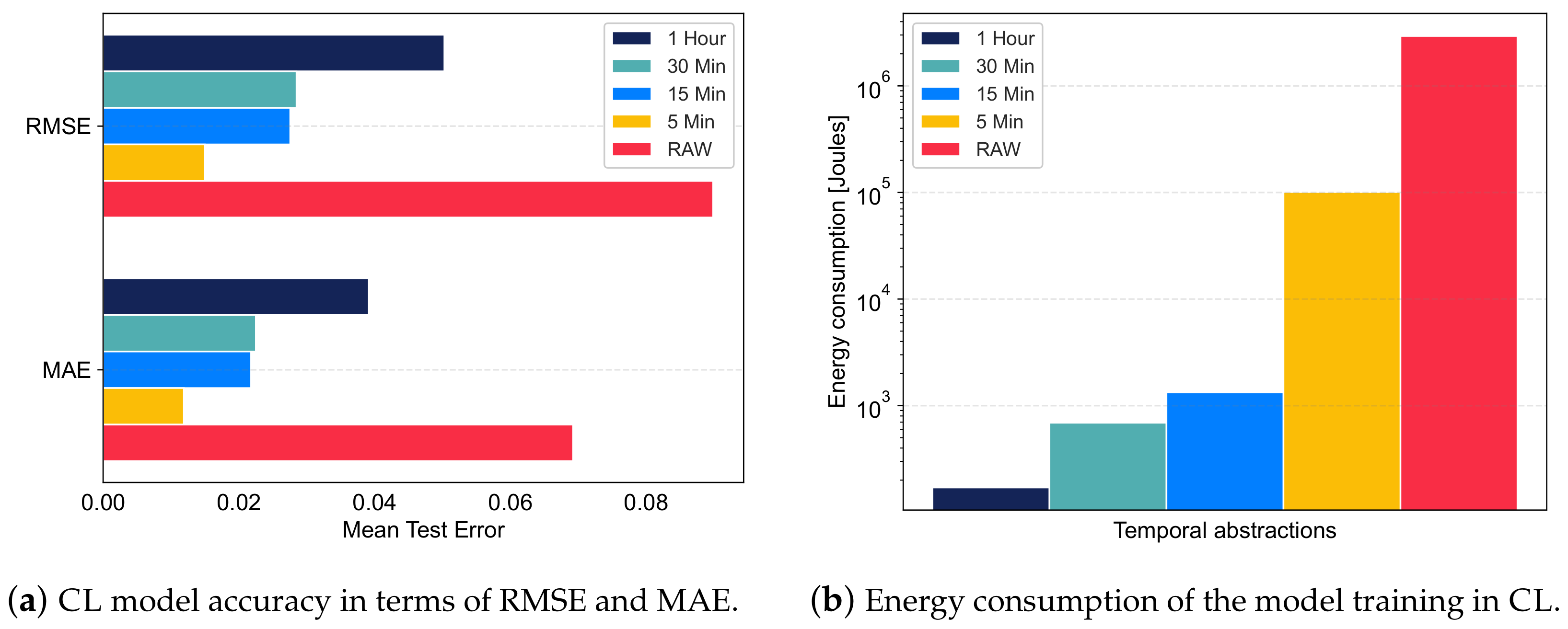
5.2.1. Impact of Temporal Abstraction

In this set of experiments, we evaluated the efficacy of our proposed temporal abstraction in terms of model performance and the energy consumption needed to accurately train thermal models. Figure 3a,b report the RMSE and MAE performance metrics (formally defined in Section 4.4) alongside the energy consumption of the trained model in CL, using the selected temporal abstraction scenarios of “1 Hour”, “30 Min”, “15 Min” and “5 Min”, compared to the “RAW” scenario, representing traditional thermal model training. Remarkably, all abstraction scenarios outperformed the “RAW” scenario both in terms of RMSE and MAE, while also using significantly less energy consumption. The “15 Min” and “30 Min” scenarios resulted in a balanced trade-off between accuracy and energy efficiency, enabling accurate yet energy-efficient thermal model training. Figure 4a indicates the total energy consumed during the thermal model training with and without considering temporal abstraction across three learning schemes (CL, FL, and PePTM). It is worth noting that traditional training corresponds to the “RAW” scenario for CL and the “5 Min” scenario for FL, where training is done using the whole dataset, with no temporal abstraction. The results show that CL required significantly more energy, whereas PePTM (even without temporal abstraction) could train personalized thermal models in an extremely energy-efficient way, as PePTM can be executed on low-power mobile devices without requiring a power-hungry server. Furthermore, the execution time required to train the thermal models can be substantially reduced when temporal abstraction is considered. For instance, in the context of PePTM, the model training with 1 hour abstraction required 93% less time compared to training without abstraction, as highlighted in

Table 2. Run time of PePTM, running for 300 rounds under different temporal abstraction scenarios.

Temporal Abstraction	1 Hour	30 Min	15 Min	5 Min
Execution time (seconds)	629 (7%)	1343 (15%)	2518 (28%)	8821 (100%)

.

5.2.2. Impact of Home Clustering

Grouping homes into clusters of similar homes allows the training of a single thermal model representative of all homes within the cluster. Figure 4b reports the RMSE accuracy of thermal models trained with and without using home clustering. Except for the “RAW” scenario in CL, where clustering resulted in data redundancy (i.e., overfitting), all other experiments in CL and FL resulted in training better models when clustering was taken into account. Although possible, using this clustering technique for PePTM results in a fully connected graph of homes, which can be costly in terms of the network bandwidth and computational updates.

Figure 4. Accuracy and energy consumption of thermal model training with and without using our proposed temporal and spatial abstraction techniques under CL, FL, and PePTM. (a) Accuracy of thermal models using data from all homes, compared to training a thermal model for each cluster of homes. (b) Energy consumption of model training in CL, FL, and PePTM schemes without using temporal abstraction.

Figure 4. Accuracy and energy consumption of thermal model training with and without using our proposed temporal and spatial abstraction techniques under CL, FL, and PePTM. (a) Accuracy of thermal models using data from all homes, compared to training a thermal model for each cluster of homes. (b) Energy consumption of model training in CL, FL, and PePTM schemes without using temporal abstraction.

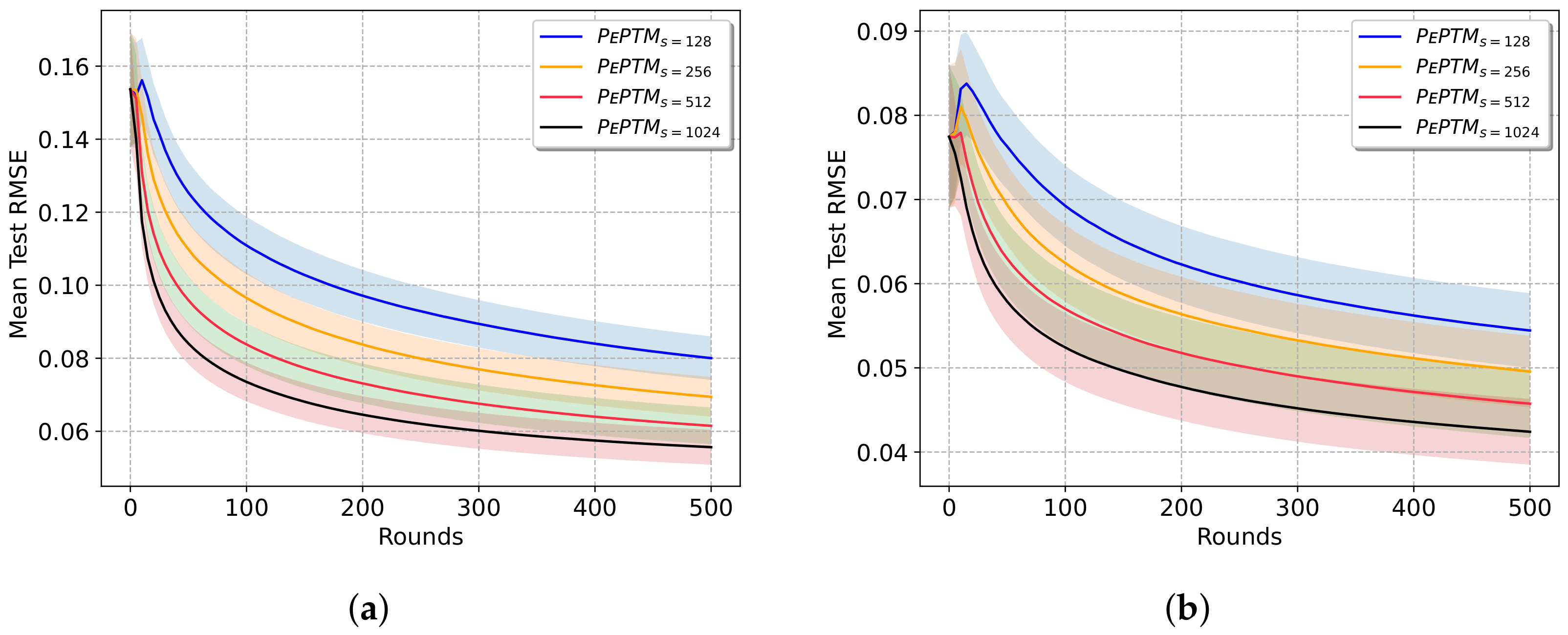
5.2.3. Configuration of PePTM

We performed several experiments to investigate the effect of varying the configuration of PePTM on model performance, energy consumption, and computational requirements. Here, we present our results and conclusions on the optimal configurations, to (1) achieve a balance between model performance and energy consumption and (2) perform model training even when using resource-constrained devices.

Convergence Rate

We configured PePTM to run between 1 and 500 rounds with an increment of 50 (i.e., 1, 50, 100, 150, …, 450, 500). To determine the optimal values for the model parameters, we conducted a set of experiments, which are presented in Figure 5a,b, for both “1 Hour” and “15 Min” scenarios, respectively, using RMSE as a performance metric. With the results shown in these figures, we found out that the optimal configuration was 300 rounds. This is because the improvements in terms of RMSE between 300 and 500 rounds are not drastic. However, energy consumption is significant.

Our experiments show that the best accuracy is reached for a batch size of 1024. However, when comparing batch sizes of 512 and 1024, the difference is not significant in accuracy, but meaningful in energy consumption. Thus, the experiments presented hereafter consider the configuration of 300 rounds with batch sizes of 128 (as a baseline) and 512. Figure 6a illustrates the RMSE performance metric of PePTM by considering the first 4 scenarios (i.e., our proposed temporal abstraction) for 300 rounds and a batch size of 512.

Figure 5. Different configurations of PePTM to determine the optimal number of rounds and sample size to achieve accurate and efficient thermal model training. The light-colored areas present the standard deviations of RMSE for the 207 homes. (a) Accuracy in terms of RMSE for PePTM, with 500 rounds and 1 h temporal abstraction. (b) Accuracy in terms of RMSE for PePTM, with 500 rounds and 15 min temporal abstraction.

Figure 5. Different configurations of PePTM to determine the optimal number of rounds and sample size to achieve accurate and efficient thermal model training. The light-colored areas present the standard deviations of RMSE for the 207 homes. (a) Accuracy in terms of RMSE for PePTM, with 500 rounds and 1 h temporal abstraction. (b) Accuracy in terms of RMSE for PePTM, with 500 rounds and 15 min temporal abstraction.

Network Density

The density of the network is a crucial configuration parameter of the PePTM algorithm. This parameter defines the average number of neighbors for each home, and directly impacts the performance of the thermal model. The more neighbors a home has, the more accurate the learned thermal model will be, thanks to the collaborative learning phase of PePTM. However, this will also increase energy consumption during this phase. Figure 6b shows the accuracy in terms of RMSE when considering different values of graph density $\rho$. The results indicate that a value of $\rho =0.05$ (about 10 neighbors) enables homes to collaborate with a sufficiently small number of similar homes, resulting in better training of thermal models compared to clustering. Moreover, having a small number of neighbors leads to significant energy savings during the PePTM collaborative training phase compared to using large values of $\rho$ or clustering. Consequently, we have chosen the value of $\rho =0.05$ to initialize the network graph of PePTM, with each home having an average of 10 neighbors.

Figure 6. Different configurations of PePTM to determine the optimal number of rounds and sample size to achieve accurate and efficient thermal model training. The light-colored areas present the standard deviation of RMSE for the 207 homes. (a) Accuracy in terms of RMSE for PePTM with 300 rounds, using a batch size of $s=512$ and graph density of $\rho =0.05$. (b) Accuracy in terms of RMSE for PePTM using different values of graph density $\rho$.

Figure 6. Different configurations of PePTM to determine the optimal number of rounds and sample size to achieve accurate and efficient thermal model training. The light-colored areas present the standard deviation of RMSE for the 207 homes. (a) Accuracy in terms of RMSE for PePTM with 300 rounds, using a batch size of $s=512$ and graph density of $\rho =0.05$. (b) Accuracy in terms of RMSE for PePTM using different values of graph density $\rho$.

5.3. Accuracy and Efficiency of PePTM

In this section, we present the achieved performance and energy consumption results of CL, FL, and PePTM. We used the described clustering methodology for CL and FL, and reported the results for cluster 0, comprising a total of 207 homes. For PePTM, we generated a network graph of 207 homes by constructing a similarity matrix with a density parameter $\rho =0.05$, resulting in each home having an average of 10 neighbors.

5.3.1. Model Performance

Figure 7a,b present the performances of the trained RNN-based thermal models under the three learning schemes, using the suggested temporal abstraction scenarios. Additionally, we trained the thermal models using only local learning (LL), where each home independently trains its thermal model locally for five complete epochs ($e=5$) without communicating with other homes. This serves to underscore the importance of the collaborative learning phase of PePTM in enhancing the accuracy of the trained models.

As PePTM allows each home to learn its own personalized model, the bars with solid colors represent the best accuracy values that homes achieved on average, and the dashed bars represent the standard deviations of the accuracy values. Figure 7a,b clearly illustrate that when homes opt for local training of their thermal models, they typically learn much worse thermal models in comparison to the other learning schemes. This observation holds true across all the considered temporal abstraction scenarios. The large dashed bars in LL indicate that homes with sufficient training data and computational resources can learn accurate thermal models. However, the majority of homes will struggle to train a satisfactory thermal model locally.

The major aspect of PePTM is that it enables these homes to collaborate and achieve better thermal models collectively by exchanging model updates, using a small number of data records that even homes with newly installed smart thermostats can obtain after a few hours of operation. Depending on the chosen sample size, PePTM can perform more computations, resulting in better thermal models, as seen with PePTM_{s = 128} and PePTM_{s = 512}. Moreover, implementing larger abstraction intervals (e.g., “30 Min” scenario) can considerably decrease the computational and energy requirements for thermal model training, particularly for homes using resource-constrained devices, at the expense of minor reductions in model accuracy, as shown in both figures.

Except for the “1 Hour” scenario, PePTM yielded slightly worse thermal models on average in comparison to CL and FL. This outcome is expected for CL, as the central server collects data from all 207 homes and trains a single thermal model accordingly. It is noteworthy to mention that we trained the thermal models for the CL scheme using the traditional training method (“RAW” scenario), and it resulted in the worst thermal model performance for both RMSE and MAE (see Figure 3a). In contrast, homes in FL update the global model using the entire dataset for each round, whereas PePTM uses a limited number of samples (to accommodate homes with less capable devices for training) and aims to reduce the training energy requirement. Nonetheless, many homes in PePTM perform better than FL, using much less training data, while other homes (around 25 out of 207 homes, according to our experiments) perform much worse, resulting in a high standard deviation (as indicated by the dashed bars).

Figure 7. Performance results in terms of RMSE (a) and MAE (b) of training an RNN thermal model in CL, FL, and PePTM, using different temporal abstractions.

Figure 7. Performance results in terms of RMSE (a) and MAE (b) of training an RNN thermal model in CL, FL, and PePTM, using different temporal abstractions.

5.3.2. Energy Consumption

In this set of experiments, we evaluate the energy consumption of the RNN model training for the three proposed temporal scenarios (“1 Hour”, “30 Min”, and “15” Min) and the “5 Min” scenario, representing the natural intervals for FL and PePTM, and the interval averaging of data received from homes in CL. For PePTM, both the default ($s=128$) and the optimal ($s=512$) batch sizes are showcased, while in the case of FL, we differentiate between the energy consumed by the server ($F{L}_{server}$) and mobile devices ($F{L}_{devices}$). It is important to indicate that despite the small energy consumption bars for FL devices in Figure 8 (due to the logarithmic scale of the Y-axis), it is still significant. For example, in the “15 Min” scenario, the energy consumed by $F{L}_{server}$ was 49,208 Joules, while $F{L}_{devices}$ consumed 13,301 Joules. In the same scenario, $PePT{M}_{s=512}$ consumed only 2182 Joules.

Figure 8 reports the energy consumption of the different experiments carried out. When comparing PePTM against CL (this comparison is not relevant: CL has an inherent single point of failure (SPoF) and privacy issues, but not PePTM), except for the “1 Hour” scenario (where CL has a slight advantage over PePTM with a batch size of 128), PePTM consistently demonstrates superior efficiency in training the thermal models compared to CL across all other scenarios (both for batch sizes 128 and 512), especially for the “5 Min” scenario, where the difference is extremely significant. Comparing PePTM against FL (this comparison is relevant because both learning approaches have the same advantages with respect to data privacy), for all considered scenarios, PePTM is extremely energy efficient. It is worth highlighting the substantial energy consumption of the mobile devices (dashed boxes in Figure 8) in FL, compared to the ones of PePTM.

Figure 8. Energy consumption of training an RNN thermal model in CL, FL, and PePTM using different temporal abstractions. Note that the y-axis is on a logarithmic scale, as the energy use of CL and FL is significantly larger than that of PePTM.

Figure 8. Energy consumption of training an RNN thermal model in CL, FL, and PePTM using different temporal abstractions. Note that the y-axis is on a logarithmic scale, as the energy use of CL and FL is significantly larger than that of PePTM.

5.4. Discussion

In this work, we introduce PePTM for training accurate and personalized thermal models for individual homes, optimizing the operation of their HVAC systems. This has the potential to significantly reduce the energy consumption of buildings on a larger scale. Furthermore, our experiments confirm the faster convergence rate and improved energy efficiency achieved through thermal model training with PePTM, resulting in further reductions in the energy footprint of buildings. The traditional training method (i.e., the “RAW” scenario) for the CL scheme achieves the worst results, both in terms of energy consumption and performance metrics of RMSE and MAE. However, CL has an edge over FL and PePTM when the thermal models are trained using our proposed temporal abstractions, and becomes the most accurate approach when models are trained according to our proposed “5 Min” scenario. Having said that, CL suffers from two fundamental issues, namely having a single point of failure (SPoF) and privacy loss. Thus, the comparison between PePTM and FL is more meaningful since both approaches protect data privacy, although FL still has the SPoF problem.

Comparing PePTM against FL, we conclude that PePTM is the best scheme from the energy consumption and accuracy perspectives. The former is due to the use of low-powered ARM-based mobile devices without requiring a power-hungry central server, which is the case for FL. Turning to the accuracy metrics (RMSE and MAE), the PePTM algorithm is slightly better than FL (on an average of 207 homes). We remark that the accuracy of the PePTM algorithm can be further improved by considering larger batch sizes. This would increase the energy consumption, but it would still be significantly more energy-efficient than FL. The same conclusions can be derived when running the three considered schemes of CL, FL, and PePTM by assuming the state-of-the-art LSTM approach for training thermal models [40]. Thus, we conjecture that the improvements in terms of energy efficiency and accuracy of our PePTM with respect to CL and FL are due to (1) our proposed temporal abstraction technique in combination with the adoption of the peer-to-peer learning scheme and (2) the usage of energy-efficient mobile phones for training instead of the power-hungry central server, which is the case for CL and FL.

6. Conclusions

Smart thermostats equipped with machine learning thermal models hold immense potential for reducing the energy consumption of buildings by optimizing the heating and cooling system operations. However, training a global thermal model for all homes using traditional centralized (CL) and federated (FL) learning schemes proves inadequate as building characteristics vary greatly. In this paper, we introduce PePTM, a personalized peer-to-peer thermal modeling algorithm designed to efficiently train personalized home thermal models in a peer-to-peer fashion without relying on a central entity, ensuring enhanced data privacy and eliminating the need for power-hungry server machines that may fail or be compromised. Our goal in this work is to achieve accurate and personalized thermal models with a minimal training energy footprint. To accomplish this, in conjunction with PePTM, we utilize two abstraction techniques: (1) temporal abstraction to downsample thermostat sensor data to larger time intervals, resulting in faster model training that can run on commodity devices, such as mobile phones; and (2) spatial abstraction to group homes with similar characteristics (e.g., floor area, age) into clusters for CL and FL, or connect homes to a small set of similar neighbors in a sparse network graph in the case of PePTM to achieve personalized thermal models while optimizing network bandwidth usage. Our experimental results demonstrate the potential of PePTM as a promising approach for efficiently training personalized thermal models in a decentralized manner, making it a suitable candidate for energy-efficient and accurate smart heating and cooling systems. In future research, we plan to assess the scalability of PePTM for larger networks of smart homes and extend its capabilities to support dynamic networks while addressing potential security and privacy challenges in the peer-to-peer setting.

References

1. Tran, Q.B.H.; Chung, S.T. Smart Thermostat based on Machine Learning and Rule Engine. J. Korea Multimed. Soc. 2020, 23, 155–165. [Google Scholar]
2. Ali, S.; Yusuf, Z. Mapping the Smart-Home Market. Tech. Rep.. 2018. Available online: https://web-assets.bcg.com/img-src/BCG-Mapping-the-Smart-Home-Market-Oct-2018_tcm9-204487.pdf (accessed on 7 August 2023).
3. Yu, D.; Abhari, A.; Fung, A.S.; Raahemifar, K.; Mohammadi, F. Predicting indoor temperature from smart thermostat and weather forecast data. In Proceedings of the Communications and Networking Symposium, Baltimore, MD, USA, 15–18 April 2018; pp. 1–12. [Google Scholar]
4. Ayan, O.; Turkay, B. Smart thermostats for home automation systems and energy savings from smart thermostats. In Proceedings of the 2018 6th International Conference on Control Engineering & Information Technology (CEIT), Istanbul, Turkey, 25–27 October 2018; IEEE: Piscataway, NJ, USA, 2018; pp. 1–6. [Google Scholar]
5. Crawley, D.B.; Lawrie, L.K.; Pedersen, C.O.; Winkelmann, F.C. Energy plus: Energy simulation program. ASHRAE J. 2000, 42, 49–56. [Google Scholar]
6. Khan, M.E.; Khan, F. A comparative study of white box, black box and grey box testing techniques. Int. J. Adv. Comput. Sci. Appl. 2012, 3, 1–141. [Google Scholar]
7. Hossain, M.M.; Zhang, T.; Ardakanian, O. Identifying grey-box thermal models with Bayesian neural networks. Energy Build. 2021, 238, 110836. [Google Scholar] [CrossRef]
8. Leprince, J.; Madsen, H.; Miller, C.; Real, J.P.; van der Vlist, R.; Basu, K.; Zeiler, W. Fifty shades of grey: Automated stochastic model identification of building heat dynamics. Energy Build. 2022, 266, 112095. [Google Scholar] [CrossRef]
9. Di Natale, L.; Svetozarevic, B.; Heer, P.; Jones, C. Physically Consistent Neural Networks for building thermal modeling: Theory and analysis. Appl. Energy 2022, 325, 119806. [Google Scholar] [CrossRef]
10. Vallianos, C.; Athienitis, A.; Delcroix, B. Automatic generation of multi-zone RC models using smart thermostat data from homes. Energy Build. 2022, 277, 112571. [Google Scholar] [CrossRef]
11. Mustafaraj, G.; Lowry, G.; Chen, J. Prediction of room temperature and relative humidity by autoregressive linear and nonlinear neural network models for an open office. Energy Build. 2011, 43, 1452–1460. [Google Scholar] [CrossRef]
12. Mba, L.; Meukam, P.; Kemajou, A. Application of artificial neural network for predicting hourly indoor air temperature and relative humidity in modern building in humid region. Energy Build. 2016, 121, 32–42. [Google Scholar] [CrossRef]
13. Xu, C.; Chen, H.; Wang, J.; Guo, Y.; Yuan, Y. Improving prediction performance for indoor temperature in public buildings based on a novel deep learning method. Build. Environ. 2019, 148, 128–135. [Google Scholar] [CrossRef]
14. Martínez Comesaña, M.; Febrero-Garrido, L.; Troncoso-Pastoriza, F.; Martínez-Torres, J. Prediction of building’s thermal performance using LSTM and MLP neural networks. Appl. Sci. 2020, 10, 7439. [Google Scholar] [CrossRef]
15. Huchuk, B.; Sanner, S.; O’Brien, W. Comparison of machine learning models for occupancy prediction in residential buildings using connected thermostat data. Build. Environ. 2019, 160, 106177. [Google Scholar] [CrossRef]
16. San Miguel-Bellod, J.; González-Martínez, P.; Sánchez-Ostiz, A. The relationship between poverty and indoor temperatures in winter: Determinants of cold homes in social housing contexts from the 40 s–80 s in Northern Spain. Energy Build. 2018, 173, 428–442. [Google Scholar] [CrossRef]
17. Vanhaesebrouck, P.; Bellet, A.; Tommasi, M. Decentralized Collaborative Learning of Personalized Models over Networks. In Proceedings of the Artificial Intelligence and Statistics (AISTATS), Lauderdale, FL, USA, 20–22 April 2017. [Google Scholar]
18. Boubouh, K.; Boussetta, A.; Benkaouz, Y.; Guerraoui, R. Robust P2P Personalized Learning. In Proceedings of the 2020 International Symposium on Reliable Distributed Systems (SRDS), Shanghai, China, 21–24 September 2020; IEEE: Piscataway, NJ, USA, 2020; pp. 299–308. [Google Scholar]
19. International Energy Agency. Buildings. 2022. Available online: https://www.iea.org/reports/buildings (accessed on 8 August 2023).
20. Pérez-Lombard, L.; Ortiz, J.; Pout, C. A review on buildings energy consumption information. Energy Build. 2008, 40, 394–398. [Google Scholar] [CrossRef]
21. Crawley, D.B.; Lawrie, L.K.; Winkelmann, F.C.; Buhl, W.F.; Huang, Y.J.; Pedersen, C.O.; Strand, R.K.; Liesen, R.J.; Fisher, D.E.; Witte, M.J.; et al. EnergyPlus: Creating a new-generation building energy simulation program. Energy Build. 2001, 33, 319–331. [Google Scholar] [CrossRef]
22. Patil, S.; Tantau, H.; Salokhe, V. Modelling of tropical greenhouse temperature by auto regressive and neural network models. Biosyst. Eng. 2008, 99, 423–431. [Google Scholar] [CrossRef]
23. Bacher, P.; Madsen, H. Identifying suitable models for the heat dynamics of buildings. Energy Build. 2011, 43, 1511–1522. [Google Scholar] [CrossRef]
24. Hossain, M.M.; Zhang, T.; Ardakanian, O. Evaluating the Feasibility of Reusing Pre-Trained Thermal Models in the Residential Sector. In Proceedings of the 1st ACM International Workshop on Urban Building Energy Sensing, Controls, Big Data Analysis, and Visualization, UrbSys’19, New York, NY, USA, 13–14 November 2019; ACM: New York, NY, USA, 2019; pp. 23–32. [Google Scholar]
25. Gouda, M.; Danaher, S.; Underwood, C. Building thermal model reduction using nonlinear constrained optimization. Build. Environ. 2002, 37, 1255–1265. [Google Scholar] [CrossRef]
26. Mtibaa, F.; Nguyen, K.K.; Azam, M.; Papachristou, A.; Venne, J.S.; Cheriet, M. LSTM-based indoor air temperature prediction framework for HVAC systems in smart buildings. Neural Comput. Appl. 2020, 32, 17569–17585. [Google Scholar] [CrossRef]
27. McMahan, H.B.; Moore, E.; Ramage, D.; Hampson, S.; y Arcas, B.A. Communication-Efficient Learning of Deep Networks from Decentralized Data. In Proceedings of the Artificial Intelligence and Statistics (AISTATS), Lauderdale, FL, USA, 20–22 April 2017. [Google Scholar]
28. Bellet, A.; Guerraoui, R.; Taziki, M.; Tommasi, M. Personalized and Private Peer-to-Peer Machine Learning. In Proceedings of the Artificial Intelligence and Statistics (AISTATS), Playa Blanca, Lanzarote, 9–11 April 2018. [Google Scholar]
29. Zantedeschi, V.; Bellet, A.; Tommasi, M. Fully Decentralized Joint Learning of Personalized Models and Collaboration Graphs. In Proceedings of the International Conference on Artificial Intelligence and Statistics (AISTATS), Palermo, Sicily, 26–28 August 2020. [Google Scholar]
30. Basmadjian, R.; Boubouh, K.; Boussetta, A.; Guerraoui, R.; Maurer, A. On the advantages of P2P ML on mobile devices. In Proceedings of the Thirteenth ACM International Conference on Future Energy Systems, Virtual Event, 28 June–1 July 2022; pp. 338–353. [Google Scholar]
31. Vyzovitis, D.; Napora, Y.; McCormick, D.; Dias, D.; Psaras, Y. GossipSub: Attack-resilient message propagation in the filecoin and eth2. 0 networks. arXiv 2020, arXiv:2007.02754. [Google Scholar]
32. Cousot, P.; Cousot, R. Abstract interpretation: Past, present and future. In Proceedings of the Joint Meeting of the Twenty-Third EACSL Annual Conference on Computer Science Logic (CSL) and the Twenty-Ninth Annual ACM/IEEE Symposium on Logic in Computer Science (LICS), Vienna, Austria, 14–18 July 2014; pp. 1–10. [Google Scholar]
33. Joshi, K.D.; Nalwade, P. Modified k-means for better initial cluster centres. Int. J. Comput. Sci. Mob. Comput. 2013, 2, 219–223. [Google Scholar]
34. Pathak, N.; Foulds, J.; Roy, N.; Banerjee, N.; Robucci, R. A bayesian data analytics approach to buildings’ thermal parameter estimation. In Proceedings of the Tenth ACM International Conference on Future Energy Systems, Phoenix, AZ, USA, 25–28 June 2019. [Google Scholar]
35. Boubouh, K.; Basmadjian, R. Power Profiler: Monitoring Energy Consumption of ML Algorithms on Android Mobile Devices. In Proceedings of the Companion Proceedings of the 14th ACM International Conference on Future Energy Systems, e-Energy ’23 Companion, New York, NY, USA, 20–23 June 2023. [Google Scholar] [CrossRef]
36. Basmadjian, R.; Shaafieyoun, A. ARIMA-based Forecasts for the Share of Renewable Energy Sources: The Case Study of Germany. In Proceedings of the 2022 3rd International Conference on Smart Grid and Renewable Energy (SGRE), Doha, Qatar, 20–22 March 2022; pp. 1–6. [Google Scholar] [CrossRef]
37. Basmadjian, R.; Shaafieyoun, A.; Julka, S. Day-Ahead Forecasting of the Percentage of Renewables Based on Time-Series Statistical Methods. Energies 2021, 14, 7443. [Google Scholar] [CrossRef]
38. Basmadjian, R.; De Meer, H. A Heuristics-Based Policy to Reduce the Curtailment of Solar-Power Generation Empowered by Energy-Storage Systems. Electronics 2018, 7, 349. [Google Scholar] [CrossRef]
39. Luo, N.; Hong, T. Ecobee Donate Your Data 1000 Homes in 2017; Pacific Northwest National Lab. (PNNL): Richland, WA, USA; Lawrence Berkeley National Lab. (LBNL): Berkeley, CA, USA, 2022. [Google Scholar] [CrossRef]
40. Boubouh, K.; Basmadjian, R.; Ardakanian, O.; Maurer, A.; Guerraoui, R. Efficient and Accurate Peer-to-Peer Training of Machine Learning Based Home Thermal Models. In Proceedings of the 14th ACM International Conference on Future Energy Systems, e-Energy ’23, New York, NY, USA, 20–23 June 2023; pp. 524–529. [Google Scholar] [CrossRef]
Figure 2. Graphical presentation of the considered centralized (left) and distributed (right) approaches. The latter case is used to conduct experiments for Federated (left) and Peer-to-Peer (right) Learning schemes. In both schemes, worker nodes are implemented in the form of mobile devices.
Energies 16 06594 g002
Figure 3. Accuracy and energy consumption of thermal model training under CL using different temporal abstraction scenarios.
Energies 16 06594 g003