Abstract
Naturally fractured reservoirs are characterized by their complex nature due to the existence of natural fractures and fissures within the rock formations. These fractures can significantly impact the flow of fluids within the reservoir, making it difficult to predict and manage production. Therefore, efficient production from such reservoirs requires a deep understanding of the flow behavior via the integration of various geological, geophysical, and engineering data. Additionally, advanced simulation models can be used to predict reservoir behavior under different production scenarios and aid in decision making and effective management. Accordingly, this study presents a robust mathematical two-phase fluid flow model (FRACSIM) for the simulation of the flow behavior of naturally fractured reservoirs in a 3D space. The mathematical model is based on the finite element technique and implemented using the FORTRAN language within a poro-elastic framework. Fractures are represented by triangle elements, while tetrahedral elements represent the matrix. To optimize computational time, short to medium-length fractures adopt the permeability tensor approach, while large fractures are discretized explicitly. The governing equations for poro-elasticity are discretized in both space and time using a standard Galerkin-based finite element approach. The stability of the saturation equation solution is ensured via the application of the Galerkin discretization method. The 3D fracture model has been verified against Eclipse 100, a commercial software, via a well-test case study of a fractured basement reservoir to ensure its effectiveness. Additionally, the FRACSIM software successfully simulated a laboratory glass bead drainage test for two intersected fractures and accurately captured the flow pattern and cumulative production results. Furthermore, a sensitivity study of water injection using an inverted five-spot technique was tested on FRACSIM to assess the productivity of drilled wells in complex fractured reservoirs. The results indicate that FRACSIM can accurately predict flow behavior and subsequently be utilized to evaluate production performance in naturally fractured reservoirs.
1. Introduction
Complexity is the rule rather than the exception in naturally fractured reservoirs, which are defined by the presence of natural fractures and fissures within the underlying formations. These fractures can significantly impact the flow of fluids within the reservoir, making it difficult to predict and manage production. Therefore, a thorough comprehension of the flow behavior is required for efficient production from such reservoirs, which can be achieved via the integration of multiple geological, geophysical, and engineering data.
The numerical modeling of naturally fractured reservoirs poses a real challenge to reservoir modelers due to the complex geological nature and the associated uncertainties in the characterization of existing fractures (i.e., the fracture attributes such as fracture network density, orientation, and mechanical properties). The presence of natural fractures plays an important role in the ultimate recovery and has a great effect on the reservoir performance; however, it is computationally expensive (if not technically infeasible) to take into account all fractures or fracture networks in standard reservoir simulators. Therefore, many studies have been published in the literature to propose different techniques on how to represent the natural fractures in reservoir simulators [1,2,3,4,5,6,7,8,9,10,11,12,13,14,15,16,17,18,19,20]. These studies can be divided into three groups based on how they account for the presence of natural fractures: 1—the dual continuum approach, 2—the discrete fracture network, and 3—the hybrid approach.
In the dual continuum approach, the matrix and fractures are two separate continua, where the matrix is considered the primary medium. The matrix–fracture media interact with each other via transfer functions that control their cross-flow and fluid exchange [21,22,23,24]. The main drawback of this approach is that it assumes an extremely simple geometrical representation of matrix and fracture.
In the discrete fracture approach, each fracture and matrix are discretized as 3D tetrahedral elements for matrix and triangle elements in a 2D space for fractures. The mathematical flow equation via matrix and fracture is modeled using various numerical approaches, such as finite element, finite volume methods, mixed finite element, and boundary element methods.
The discrete fracture approach has many advantages, such as the explicit representation of individual fractures on fluid flow and the approach not being constrained by grid fracture geometries; moreover, the fracture model is easily adjustable, and the fluid exchange between the matrix and fracture depends on the fracture geometry, relative permeability, and capillary pressure functions. Nevertheless, the main disadvantage of this approach is the complexities associated with the implementation process and the computational cost (i.e., the discretization of fractures in the created mesh requires local refinement and will most likely increase the computational time). To overcome such limitations, a hybrid approach was adopted by many researchers [25,26,27,28,29]. In this approach, the concept of effective permeability tensor is adopted, where the fractures are partitioned into short and long fractures depending on the cut-off value determined via the reservoir modeler. Each block with short fractures is replaced with a homogenous grid block with an equivalent 3D permeability tensor (i.e., the short fractures are considered local spatial heterogeneities within the matrix block). On the other hand, the long fractures are explicitly discretized and coupled with the 3D permeability tensor matrix.
The main objective of this study is to provide a simulation tool for discrete fracture media using the finite element method (FEM) for simulating two-phase fluid flow in a coupled poro-elastic framework. The simulation of the discrete fractured system contains the interaction of two domains: the first domain is the porous medium, and the second one is the fractures. In this study, the concept of effective permeability tensor to calculate the 3D equivalent permeability of matrix and fractures for small to medium fractures is used to save computational time by imposing the fracture elements into the matrix elements, whereas large fractures are discretized explicitly. In this model, fractures are discretized using triangle elements, while the matrix is represented by tetrahedral elements. The poro-elastic governing equations are discretized in space and time using a standard Galerkin-based finite element approach. The solution of the saturation equation in the finite element approach is stabilized using the Galerkin discretization method. The structure of this study is as follows: the derivation of the proposed coupled poro-elastic mathematical model is presented in Section 2. Then, the validation of the in-house simulator against (1) an exact analytical solution of a 2D poro-elasticity problem (Kirsch’s Problem), (2) a 3D lab-scale drainage test of fractured micro-glass bead, and (3) history matching of real field dynamic data (well-test data) of a fractured basement reservoir are presented in Section 3 of this study. Finally, the conclusions of the study findings are presented in Section 4.
2. Derivation of Multiphase Flow Equations
2.1. Mass Conversation Equation
In porous media, the solid mass is represented as
ρs and ϕ are the density of solid constituents and sum of fracture–matrix porosity, respectively.
The conservation of solid mass in porous media can be written as
Under continuum mechanism, Equation (2) is simplified to
In the same manner, the fluid mass conversation (i.e., the two phases of mass: oil and water) inside the matrix–fracture systems can be presented as follows:
Two-phase fluid mass:
In terms of fluid constituents Equation (4) will be as follows:
In Equation (5), ρ, S, and q are fluid density, fluid saturation, and the fluid exchange rate between the matrix and fracture systems. Also, refers to fluid phase (water or oil).
Assuming the existence of continuum state, Equation (5) can be written in terms of oil and water as follows:
where U is the intrinsic fluid velocity.
where is the matrix permeability, is the matrix pressure, and is the fracture pressure.
The matrix and fracture Darcy’s velocity in terms of oil and water is written as
By re-arranging Equation (9), the two-phase intrinsic velocity is written as
Using the intrinsic oil and water velocities in Equation (10) in Equation (7) gives
The expanded form of Equations (3) and (11) are as follows [30]:
The expanded form in Equations (13) and (14) can be re-arranged as
Total derivative is defined as
Direct application of Equation (17) into Equations (15) and (16) gives
Using Equation (18), the porosity change with time can be as follows:
Substituting Equation (20) into Equation (19) gives
or
The rate of change in fluid and rock densities are related to the bulk modulus as follows:
where K is the bulk modulus, and the subscripts (o, w, and s) refer to water, oil, and rock, respectively.
Direct substitution of Equation (23) into Equation (22) will give
Equation (24) is the general form of the two-phase fluid flow equation; however, this equation can be simplified by applying the total derivative presented earlier in Equation (17), combining Equation (24) with Darcy’s law, and neglecting solid velocity considering that it is small compared to other constituents; this will give a phase velocity as follows:
where is the phase symbol (oil or water phase), and and are relative permeability and density of the phase, respectively.
Accordingly, the water flow equation is written as [30]
Pw is the water pressure, and the subscript terms (f and m) refer to the fracture and matrix systems, respectively.
Similarly, the oil phase fluid flow is as follows [30]:
2.2. Momentum Balance Equation
The total stresses in porous media can be written as a function of effective stresses as follows:
and are the Kronecker delta and the pore pressure ratio factor, respectively.
The effective stress can be written as a function of the elasticity matrix as follows:
For a certain traction vector F applied on a solid body under total stress , the equilibrium of solid motion will be as follows:
where is the vector of tractions applied on the body.
The relationship between displacement and strain can be written as follows:
2.3. Finite Element Discretization
This section gives a brief explanation of the finite element method used to simulate the coupled fluid flow and rock poro-elasticity equations. Moreover, the discretization technique of the problem domain into nodal system is also explained.
The four-node tetrahedral element presented in Figure 1 has the following shape functions in terms of local coordinate system [30]:
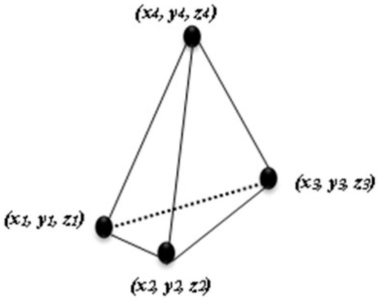
Figure 1.
Linear tetrahedral element used in a finite element calculation.
Equation (33) can be used to transform the element geometry from the global coordinates (x, y, and z) to the local coordinates as follows:
In Equation (33), the Jacobin matrix J has the following form:
To determine how the element’s unknown variables vary, shape functions are utilized. In finite element space, interpolation functions are usually used to approximate these unknowns as follows:
, , and are the elements’ unknowns, and N is the corresponding shape function.
The strain displacement matrix B is defined as
The general equilibrium equation is defined as follows:
and V are the boundary load vector and the volume of the element, respectively.
Combining Equations (39) and (40) and dividing by will give the following equation:
The average pore pressure is defined as
Inserting the pressure term in Equation (42) into Equation (41) will give
Adding the capillary pressure term to Equation (43) will give
The water flow equation inside the fracture system is discretized as follows:
Two-dimensional fluid flow inside discrete fracture is written as
where refers to the porous media domain, and the subscripts f and m refer to fracture and matrix domains.
2.4. Evaluation of Non-Linear Coefficients and Computational Procedure
In this work, the model’s unknowns have been calculated at each time step using an iterative methodology. With this method, nonlinear coefficients like capillary pressure, relative permeability, and saturations can be evaluated. The primary unknowns affect these coefficients. The most current fluid pressure computations are used to update the coefficients at each iteration level. Using the updated calculations of capillary pressures, the new values of water saturation at matrix and fracture nodes are estimated from capillary pressure and saturation relationships. Therefore, in order to arrive at a stable solution of fluid pressures and displacement, a convergence criterion is applied to Equations (44) and (45) as follows:
At each iteration number i, the convergence level of the nodal unknown R at the node number k should be less than or equal to a convergence limit ( = 0.01).
3. Results and Discussion
The verification of the presented in-house model is important to ensure that the developed 3D coupled poro-elastic concept is implemented correctly into the in-house model. Therefore, in this section, the ability of the developed model (FRACSIM) to capture the complex flow behavior of naturally fractured reservoirs under a poro-elastic environment was validated against (1) an exact analytical solution of a 2D poro-elasticity problem (Kirsch’s Problem), (2) a 3D lab-scale drainage test of fractured micro-glass bead, and (3) the history matching of real field dynamic data of a fractured basement reservoir. The discerption and analysis of each validation case will be presented next.
3.1. Validation Using Kirsch’s Problem in Poroelasticity
The Kirsch model was originally developed to estimate the tangential and radial stresses around a hole in a homogenous infinite plate under unidirectional tension and assuming a plane-strain case (Kirsch 1898) [31]. For the case of a vertical borehole in a poro-elastic environment, Detournay and Cheng 1988 [32] presented an analytical solution of the pore pressure, the stress, and the displacement induced by drilling, producing, or pressurizing the borehole. In their study, they used the Laplace space transformation to derive the analytical solution, which then was transformed to the time domain using a numerical inversion technique. Herein, we present a verification of the poro-elastic in-house model (FRACSIM) against the analytical solution presented by Detournay and Cheng for a circular-shaped reservoir (see Figure 2).
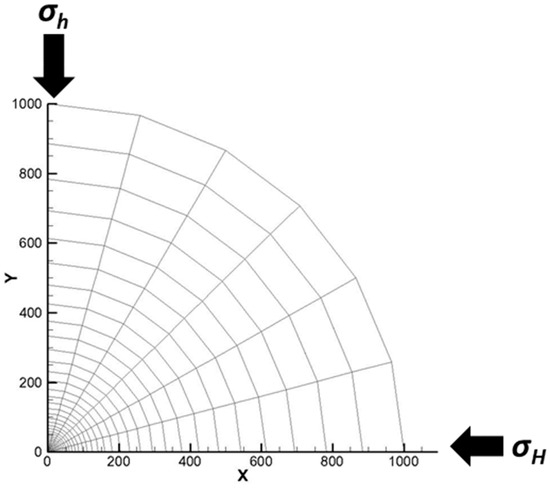
Figure 2.
Two-dimensional circular reservoir used for validation of the poro-elastic in-house model (FRACSIM) with maximum horizontal stress σH and minimum horizontal stress σh.
The pore pressure, radial stress, tangential stress, radial displacement, and tangential displacement analytical solutions of a two-dimensional model of a circular-shaped reservoir with a maximum horizontal stress σH, a minimum horizontal stress σh, an initial pore pressure Pi, a wellbore pressure Pw, a wellbore radius rw, and a drainage radius re are as follows [32]:
Pore pressure:
Radial stress:
Tangential stress:
Radial displacement:
Tangential displacement:
In Equations (48)–(52), G is Young’s modulus, v is Poisson’s ratio, η is the poro-elastic coefficient () with a physical range of variation of [0–0.5], θ is the angle relative to the direction of the maximum horizontal stress, and r is the radial distance from the borehole to the point of calculation for stresses and displacements. Moreover, the Laplace space transform of the functions g (r, t) and h (r, t) is as follows:
where K0 and K1 are the first-order modified Bessel functions of the first and second kind.
The results of the developed poro-elastic in-house simulator were compared to the analytical solution presented in Equations (48)–(53) for a 2D circular reservoir with a wellbore radius of 0.1 m and a drainage radius of 1000 m. The reservoir rock and fluid properties used in this comparison are presented in Table 1.

Table 1.
Parameters used in the verification of poro-elasticity solutions.
Figure 3 presents a comparison of the tangential stress of the analytical solution and the in-house simulator for different time steps (after one day, one month, and one year of production). It can be seen from this figure that the poro-elastic in-house model is in good agreement with the analytical solution. Furthermore, Figure 4A–C present the tangential displacement of the analytical solution and the in-house model after one day, one month, and one year of production; it is clear from this figure that the in-house code results are in close agreement with the analytical solution. It should be noted that the same level of agreement between the analytical solution and the in-house model was achieved for the radial stress and displacement for this validation exercise. Such results highlight the capability of the developed in-house model in capturing the stress redistribution and displacement due to production or pressurizing the borehole under the assumption that the rock behaves as a poro-elastic material with compressible constituents.
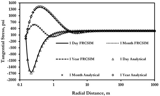
Figure 3.
Comparison of tangential stress (σθθ) of the analytical solution and the in-house simulator (FRACSIM) under σH = 5800 psi and σh = 5500 psi, Pr = 5500 psi, Pw = 1000 psi, kx = 0.01 md, and ky = 0.01 md.
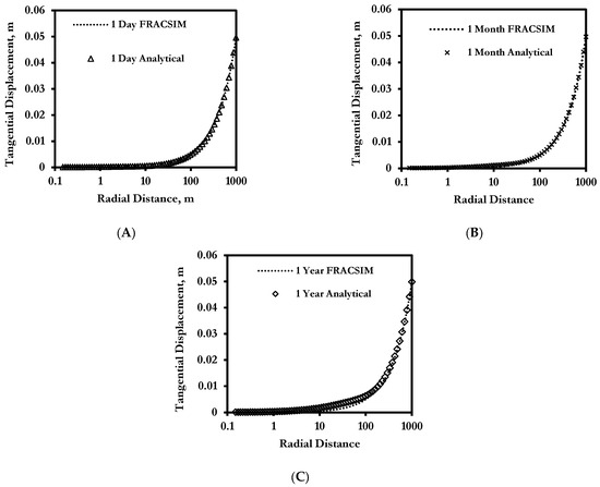
Figure 4.
Comparison of tangential displacement (uθ) of the analytical solution and the in-house simulator (FRACSIM) under σH = 5800 psi and σh = 5500 psi, Pr = 5500 psi, Pw = 1000 psi, kx = 0.01 md, and ky = 0.01 md (A) after one day of production, (B) after one month, and (C) after one year.
3.2. History Matching of Two-Phase Flow Real Data—Laboratory Scale
The visualization experiments of the two-phase flow in fractured glass bead micro-models are a good tool to observe the flow behavior of fractured media and understand the interaction between matrix and fracture system as well as to investigate the effect of fracture properties on fluid flow. In this section, the in-house poro-elastic model was used to history match a drainage test result of a 200 mm × 100 mm × 2 mm multiple fractured glass bead model reported by Fahad et al., 2012 [33]. The drainage test was conducted on a homogeneous glass bead matrix with a mesh size range of 105 to 145 µm, while the fracture was made up of thin glass strips placed at the center of the model with different fracture orientations and densities. This drainage test studied the flow around two crossed fractures placed at the center of the glass bead matrix. Figure 5 presents a schematic of the experimental setup of the glass bead model used for the multiple crossed fracture drainage test. The matrix and fracture permeabilities are 3.4 and 104 Darcy, respectively. The experiment started with saturating the glass bead matrix with water, which has a viscosity of 1.002 cp and a density of 0.998 gm/cm3. Then, a Soltrol-130 iso-paraffin oil, with a viscosity of 1.4 cp and a density of 0.75 gm/cm3, was injected at the inlet of the glass bead matrix to displace the water at a constant injection rate of 2 cc/min, effluent volume produced from the displacement process are collected at the outlet of the glass bead model. Moreover, the displacement front was recorded using a digital camera with the help of a light source that was installed underneath the glass bead model to illumine the fractured glass bead matrix.

Figure 5.
Schematic of the experimental setup of the glass bead model used for the multiple crossed fracture drainage test.
The developed in-house model was used to simulate the fractured glass bead drainage test. Figure 6A, top image, presents the generated in-house mesh to simulate the drainage experiment of two-phase flow on crossed-fractures at the center of a glass bead matrix. In this image, the tetrahedral elements of the mesh represent the matrix, while the fine triangle elements are used for meshing the two-crossed fractures. In addition, Figure 6A’s middle and bottom images represent the drainage test visualization at 0.4 pore volume injected (0.4 PVI) and the simulated drainage test using the in-house poro-elastic model at the same pore volume injected, respectively. It can be noted from Figure 6A (middle and bottom images) that the in-house simulated drainage test image is in close agreement with the experimental drainage test image at the same pore volume inject (PVI = 0.4). Furthermore, Figure 6B presents a comparison of the measured produced water volume of the drainage experiment and that from the in-house model; it can be seen from this figure that the in-house model produces an excellent match to the measured water volume from the fractured glass bead experiment. Such results clearly highlight the capability of the developed model to capture the flow behavior of fractured media at the laboratory scale with a good level of accuracy. The validation of the in-house model with real field data will be presented in the next section.

Figure 6.
((A)—Top) presents the generated in-house mesh to simulate the drainage experiment of two-phase flow on a crossed-fractures at the center of a glass bead matrix; ((A)—Middle) presents the drainage test visualization at 0.4 pore volume injected (0.4 PVI); (light blue is water, and dark red is Soltrol-130 oil); ((A)—Bottom) presents the simulated drainage test using the in-house poro-elastic model at 0.4 pore volume injected (0.4 PVI). (B) History matching the drainage test produced water volume using the in-house poro-elastic model.
3.3. History Matching of Real Dynamic Data—Field Scale
In this section, the developed in-house simulator is used to history match a well test data of a fractured granitic oil-bearing basement reservoir located in Southeast Asia using a hybrid discretization technique that couples the single continuum and the discrete fracture method in a poro-elastic environment. The hybrid approach consists of three main steps: 1—stochastic generation of 3D subsurface fracture network map based on field static data, 2—calculation of grid-based 3D permeability tensors accounting for short fractures, and 3—coupling of single continuum (grid-based permeability tensor) and explicit discrete long fractures. A brief description of the hybrid approach is given in the next paragraph.
In this study, the discrete fracture network map was generated via the statistical analysis of field data (static data) procedures developed by Doonechaly and Rahman (2012) [34]. This technique integrates different field data to determine a distribution range of fracture properties (fracture orientation, fracture density, and fractal dimension); the integrated field data include core analysis, conventional well logs, seismic attributes, and wellbore images. The determined fracture density and fractal dimension distributions are used as an input to an object-based stochastic sequential Gaussian 3D simulator to generate different random realizations of fracture attributes. In this simulation, the fractures are treated as circular disk objects, as shown in Figure 7. Each fracture is defined based on its orientation (i.e., the dip and azimuth angles of the fracture), center point (i.e., fracture location), radius, and aperture. Moreover, the random realization of fractures continues until the total fracture intensity and fractal dimension of the studied area are met. At this point, the resulting model is the 3D subsurface fracture map of the studied reservoir. Afterward, the generated 3D subsurface map is divided into a number of grid blocks (N grid blocks) in order to calculate the grid-based permeability tensors, as shown in Figure 8A. For this purpose, a threshold fracture length (LFmin) is defined. Accordingly, fractures with a length less than the threshold fracture length that cut a certain block are used to calculate the permeability tensors of that block (i.e., fractures that have a length less than (LFmin) are considered as part of the matrix in the form of permeability tensor; in other words, the short fractures are considered local spatial heterogeneities within the matrix block), as shown in Figure 8B. Once the grid-based 3D permeability tensors are calculated, the matrix domain is coupled with the explicitly discretized long fractures (i.e., fractures with fracture length > LFmin). The matrix domain is discretized using four-node tetrahedral elements, while the triangular elements are used for the discretization of explicit long fractures, as shown in Figure 8C. The used grid blocks were built using an in-house developed mesh generator. It should be noted that the grid-based permeability tensor calculations, which include diagonal and off-diagonal terms, are performed using three-dimensional Darcy’s law and continuity flow equations under pressure and flux periodic boundary conditions developed by Durlofsky (1991) [35]. Once the hybrid permeability tensor and discrete fracture mesh is ready, then it is used in the FRACSIM in-house poro-elastic model to simulate fluid flow around the fractured well and history match the dynamic production data (well test data).
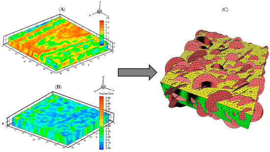
Figure 7.
(A) Three-dimensional fracture density distribution; the fracture density varies between 2.5 m−1 and 6.5 m−1. Red color indicates high fracture density. (B) Three-dimensional fractal dimension distribution; the fracture density varies between 2.5 m−1 and 6.5 m−1. (C) Stochastic realization of discrete fracture map using object-based simulator; hence, fractures are represented as circular disk objects with their unique center point, dip, azimuth, and radius.
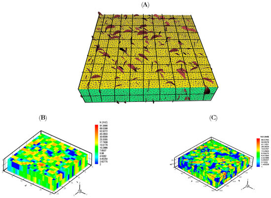
Figure 8.
Demonstration of the hybrid approach: (A) division of the reservoir into a number of grid blocks, (B) conversion of short-to-medium fractures into 3D-grid-based permeability single continuum, and (C) coupling of the grid-based permeability tensors with discrete fracture network via an explicit discretization the long fractures.
A complete algorithm of the well-test history matching process is summarized as follows:
- Generate the subsurface fracture realization using field data based on Doonechaly and Rahman (2012) approach [34].
- Utilizing periodic boundary conditions Durlofsky (1991) [35], calculate the block-based permeability tensor of the single continuum taking into account the short fractures.
- Couple the block-based permeability tensor with the discrete fracture network of long fractures using the in-house mesh generator (hybrid approach).
- Start FRACSIM in-house model to simulate pressure build-up and draw-down cycles.
- Compare the FRACSIM results with that of the measured well test data to estimate the error.
- If the error from step 5 is less than the predefined error threshold, then stop and report the optimum fracture realization with the pressure change and pressure derivative results. Otherwise, go back to step 1 to modify the fracture attribute and generate a new fracture realization. The simulated well-test results are compared with that from the build-up and draw-down test data for each realization until the error is minimized.
Accordingly, the FRACSIM numerical model with the hybrid approach is used to simulate single-phase fluid flow via the subsurface fracture realization, which was generated using field data of a fractured granitic oil-bearing formation located in Southeast Asia. According to geological interpretation, the formation is highly fractured with an extremely low matrix porosity and permeability. The network of fractures formed the majority of storage spaces in the studied formation. A Drill Stem Test (DST) was conducted in this formation with controlled flow periods before shutting to better understand the reservoir extent and evaluate well deliverability. The reservoir and fluid input data of the simulation study are presented in Table 2. Different subsurface fracture realizations were generated using the available field data. A total of 3000 fractures were created, and the minimum fracture length threshold was set to 40 m. The grid-based permeability tensors were generated accounting for fractures with a length < 40 m. Long fractures with lengths > 40 m were discretized explicitly and coupled with the single continuum. The different fracture realizations were fed to the in-house FRACSIM model to simulate the main build-up and draw-down period of the DST test. Moreover, a commercial reservoir simulator (Eclipse100) was used to simulate the build-up test and draw-down periods. However, only the grid-based permeability tensor was passed to Eclipse100 since this simulator lacks the ability to explicitly discretize fracture network. Figure 9 presents the optimum coupled permeability tensor and explicit fracture network of the simulated area.
Table 2.
Reservoir inputs data for a typical fractured basement reservoir.

Figure 9.
The optimum coupled permeability tensor and explicit fracture network of the simulated area.
Figure 10 presents the simulated shut-in pressure using FRACSIM and Eclipse100 compared to the measured shut-in pressure. It can be seen from this figure that the in-house simulator closely matches the measured shut-in pressure data. On the other hand, the Eclipse100 failed to provide a good match and underestimated the measured shut-in pressure. Similar to the in-house simulator, the simulated area in the Eclipse-100 model was divided into different grid blocks, and then the intersected fractures with each block have been accounted for in the form of permeability tensors for each grid block using the periodic boundary condition. However, the explicit discrete fracture approach represents fractures as a 2D triangle surface sandwiched between the 3D tetrahedral domain, giving it the flexibility to mesh any kind of fracture orientation and shape. Such fracture representation is not available in the ECLIPSE simulator, as the fractures were presented with the stack of grid blocks, which is the main reason that the Eclipse-100 model could not match the shut-in pressure as the effect of long fractures on pressure change is neglected. Furthermore, Figure 11 presents the simulated draw-down cycle of the DST using FRACSIM and Eclipse100 in comparison to the measured draw-down pressure. It can be noted from this that the FRACSIM produced a good match to the measured draw-down curve, while the Eclipse100 failed to match the measured draw-down pressure.
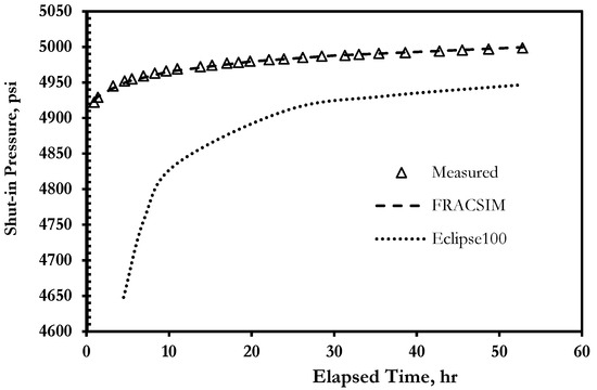
Figure 10.
The simulated shut-in pressure of FRACSIM in-house model and Eclipse100 compared to the measured shut-in pressure.
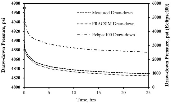
Figure 11.
The simulated draw-down profile of FRACSIM in-house model and Eclipse100 compared to the measured draw-down pressure.
Figure 12A presents the pressure change and pressure derivative of the finite-difference-based reservoir simulator ECLIPSE-100 in comparison to the pressure change and pressure derivative. It can be noted from this figure that, again, the Eclipse100 model could not match the measured pressure change and pressure derivative data as a result of ignoring the effect of long fractures. Figure 12B presents the pressure change and pressure derivative results of the FRACSIM results compared to the measured data. It is clear from this figure that the in-house model results have a good match with the measured results. Furthermore, the FRACSIM in-house model and the measured data pressure derivative curves show similar flow regimes that include the spherical flow due to partial well penetration at early time (characterized by a negative slope in the derivative curve), followed by a short radial flow at middle time (characterized by flatness in the derivative curve with a zero slope) and a late linear flow due to the effect of fractures (characterized by a positive half-slop of the derivative curve). Such encouraging results highlight the good capability of the in-house poro-elastic simulator in simulating fractured reservoirs. Finally, the in-house single well model was run for one year under a natural depletion scenario in order to visualize the change in fluid velocity and reservoir pressure in the fracture network. Figure 13A–D present the velocity profile and the pressure profile of the single well model after one month and one year of production under a constant bottom hole pressure of 2300 psi. It can be noted from this figure that the permeability of the connected discrete fractures has a significant effect on fluid velocity and reservoir pressure diffusion, almost all connected fractures exhibit a high change in velocity, especially the fractures near the wellbore at the early production time (one month), as production continues to one year the velocity change is dominant in all fractures in the studied area. The same trend is present with the pressure distribution: after one year of production, the pressure change reaches the boundary of the studied area.
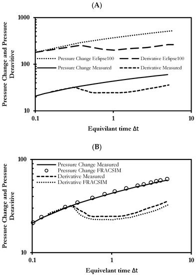
Figure 12.
(A) The pressure change and pressure derivative of the finite-difference-based reservoir simulator ECLIPSE-100 and (B) the pressure change and pressure derivative of the FRACSIM in-house model compared to measured data.
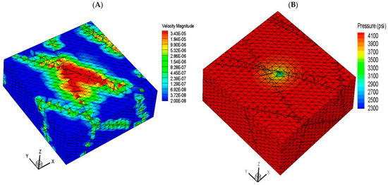
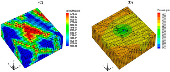
Figure 13.
(A) The velocity profile and (B) the pressure profile of the single well model after one month of production; (C) the velocity profile and (D) the pressure profile of the single well model after one year of production. The well is located at the center of the block.
3.4. Sensitivity Study of Full Field Development Plan
In this section, the developed in-house simulator was utilized to investigate the performance of the reservoir (presented in Section 3.3) under two driving mechanisms: natural depletion and water flooding. The reservoir dimension of 4000 m × 5000 m × 250 m was used in the FRACSIM simulator with the fracture realization that was verified in the previous section. The first step was to investigate the reservoir performance under volumetric natural depletion since the reservoir does not have any aquifer support. The reservoir rock and fluid properties are similar to those presented in Table 2 (Section 3.3), and the relative permeability curves are shown in Figure 14A,B. Sixteen vertical producers were placed across the reservoir (see Figure 15). These producers were run under constant bottom hole pressure of 1000 psi, with a simulation period of 15 years. Figure 16 presents the oil production rate of the highest and lowest producers among the sixteen wells after 15 years of production. From this figure, it can be seen that the well production shows a typical production behavior of fractured reservoirs; that is, the wells start with a high production rate for a short period of time then production goes in a rapid decline. This is primarily driven by the fact that fluids initially flow via fractures, which led to a significant drop in wellbore pressure with a spike in fluid production. Then, the matrix begins to feed the fracture network with fluid. During this flow period, oil production at the wellbore drops to a steady low rate with a gradual decrease in wellbore pressure. The simulation results show that Well-P16 was the highest producer among the sixteen wells with a production rate of 13,146 bbl/day at the beginning of production; then, the production rate declined to 70 bbl/day after 6 years of production. Well-P2 was the lowest producer among all with an initial production of 4400 bbl/day; then, the production decreased to 20 bbl /day after 6 years of production. It should be noted that the flow rate profiles of all other wells were bounded between the highest and lowest producer rate profiles and followed the same trend as that seen in well-P6 and Well-P2 but with different ranges of oil rates. Moreover, the water production was negligible because the simulation was run with only connate water. The cumulative oil production ranges from 1.13 × 10⁶ bbl at well-P2 to 2.98 × 10⁶ bbl at well-P16. The total oil production for the studied reservoir is 3.27 × 10⁷ bbl after a simulation of 15 years.

Figure 14.
The reservoir relative permeability cures, (A) matrix relative permeability, and (B) fracture relative permeability.
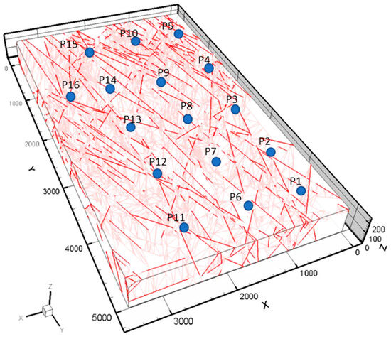
Figure 15.
The discreet fracture map with the location of the sixteen producers represented by a blue circle.
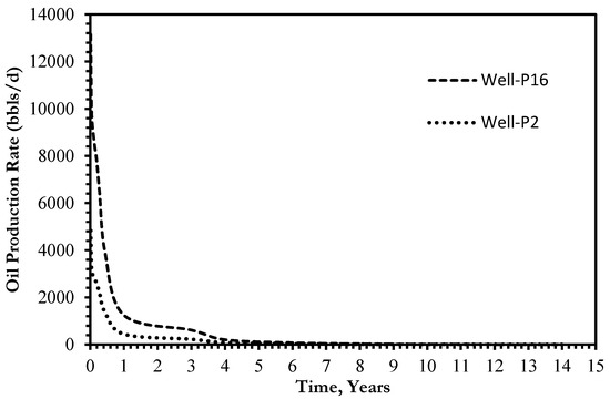
Figure 16.
The oil production rate of the highest and lowest producers among the simulated sixteen wells.
In order to investigate the reservoir performance under water flooding, wells (P3, P7, P9, and P13) were converted into injection wells; these wells were chosen as they are located at the center of the studied area, as shown in Figure 17. The amount of water injected in each well was 6000 bbl/d. The reservoir thickness is 250 m; water was injected into the bottom region (the bottom 100 m of the reservoir thickness), while the oil was produced from the reservoir top section (the top 90 m of reservoir thickness). Thus, there is around a 60 m zone separating the producing and injection sections.
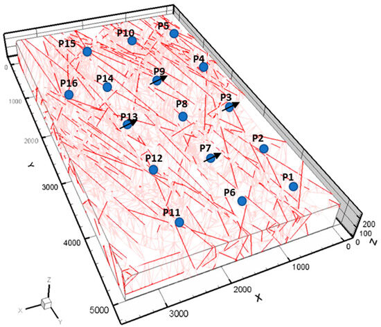
Figure 17.
The discreet fracture map with the location of the twelve producers represented by a blue circle and the four injectors (P3, P7, P9, and P13) represented by a blue circle with slanted arrow.
Figure 18, Figure 19 and Figure 20 present the oil production rate, the water cut, and the water production rates of the production wells, respectively. It can be seen from these three figures that Well-P8 has the highest oil and water production rate. This is due to the fact that Well-P8 location is bounded by four injectors, which, in turn, creates a high sweep efficiency area around Well-P8. Well-P5 has the lowest water production rate because the location of this well is far from the injection area. Furthermore, the water saturation map after one year is shown in Figure 21A, while the water saturation and pressure after five years of injection are shown in Figure 21B and Figure 22 respectively. Figure 23 presents a cumulative production chart for each producer under the natural depletion and the water flooding mechanisms. Furthermore, Table 3 presents the percentage change in each producer’s cumulative total oil production following the water flooding procedure in comparison to the cumulative total oil production due to natural depletion. It can be concluded from Figure 23 and Table 3 that all producers (except Well-P8) show a certain degree of improvement in the cumulative oil production due to water injection. For example, Wells P2, P4, P5, P6, P10, P12, and P14 show a promising percentage of improvement, reaching as high as 200% in the case of P2 and P4. The improvement in cumulative production is mainly attributed to the relative location of the well and the intensity of the fracture network intersecting that well. Wells that intersect high-intensity fractures will suffer from high water break though, such as Well-P15, which has the highest water cut among all producers. Furthermore, Well-P8 showed a reduction in total cumulative production compared to the natural depletion scenario due to the fact that it has the highest water production rate among all producers because it was bounded by four injectors. In summary, the presented results indicate that a comprehensive understanding of the geological characterization and fracture network structure via the integration of different resources including static and dynamic field data, will certainly help in achieving successful waterflooding in naturally fractured reservoirs.

Figure 18.
The oil production rate of the simulated twelve producers under water flooding.
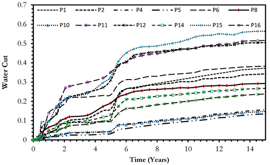
Figure 19.
The water cut of the simulated twelve producers under water flooding.
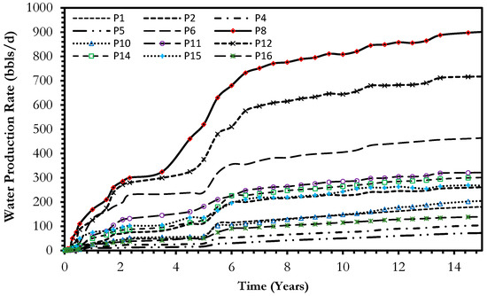
Figure 20.
The water production rate of the simulated twelve producers under water flooding.
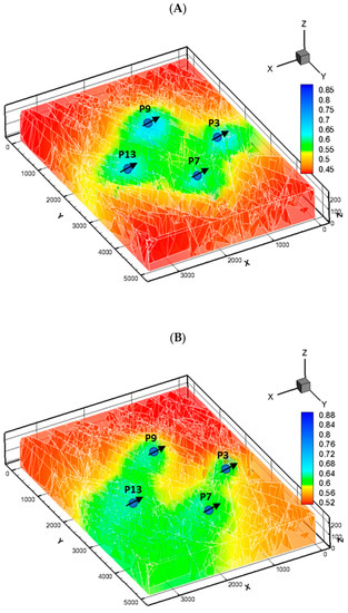
Figure 21.
The water saturation map of around the injection wells (A) after one year of water injection and (B) after five years of water injection.
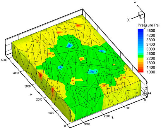
Figure 22.
The reservoir pressure map around the injection wells after five years of water injection.
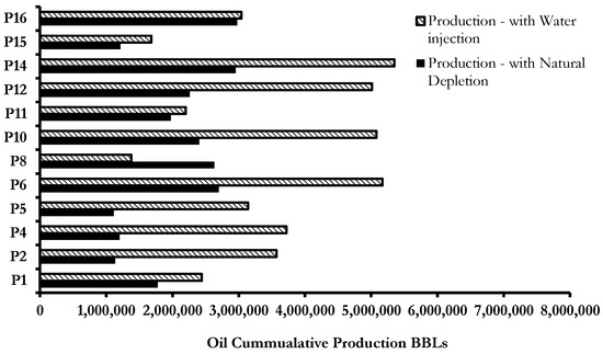
Figure 23.
Total cumulative oil production bar chart for each producer under natural depletion and water flooding mechanisms.
Table 3.
Comparison between cumulative oil production of each well before and after water injection.
3.5. Limitation and Future Work Recommendation
This presented study has a few limitations that should be considered. Firstly, it only simulates two-phase flow and does not account for other phases. Secondly, the long run time is observed for large mesh cases, particularly those with high-intensity fractures. In future research, efforts will be directed toward improving computational efficiency by employing parallel computing methods and incorporating three-phase flow equations into the model. Additionally, ongoing development aims to incorporate parameters such as thermal stresses in fractured reservoirs and the combined effects of thermal and chemical variations in fractured geothermal reservoirs.
4. Conclusions
This study presents a robust mathematical two-phase fluid flow model (FRACSIM) for the simulation of flow behavior of naturally fractured reservoirs in a 3D space. The mathematical model is based on the finite element technique and implemented using the FORTEAN language within a poro-elastic framework. Fractures are represented by triangle elements, while tetrahedral elements represent the matrix. To optimize computational time, short to medium-length fractures adopt the permeability tensor approach, while large fractures are discretized explicitly. The governing equations for poro-elasticity are discretized in both space and time using a standard Galerkin-based finite element approach. The stability of the saturation equation solution is ensured via the application of the Galerkin discretization method. The 3D fracture model has been verified against Eclipse 100, a commercial software, via a well test case study of a fractured basement reservoir to ensure its effectiveness. Additionally, the FRACSIM successfully simulated a laboratory glass bead drainage test for two intersected fractures and accurately captured the flow pattern and cumulative production results. Furthermore, a sensitivity study of water injection using an inverted five-spot technique was tested on FRACSIM to assess the productivity of drilled wells in complex fractured reservoirs. The results indicate that FRACSIM software can accurately predict flow behavior and subsequently be utilized to evaluate production performance in naturally fractured reservoirs.
Author Contributions
Conceptualization, R.A.A. and S.A.; Methodology, R.A.A.; Software, R.A.A.; Validation, S.A.; Formal analysis, S.A. and A.A.; Investigation, R.A.A. and S.A.; Resources, A.A.; Writing—original draft, R.A.A.; Writing—review & editing, S.A.; Visualization, A.A. All authors have read and agreed to the published version of the manuscript.
Funding
This research received no external funding.
Data Availability Statement
The datasets used and/or analyzed during the current study are available from the corresponding author upon reasonable request.
Conflicts of Interest
The authors declare no conflict of interest.
References
- Barenblatt, G.; Zheltov, I.; Kochina, I. Basic concepts in the theory of seepage of homogeneous liquids in fissured rocks [strata]. J. Appl. Math. Mech. 1960, 24, 1286–1303. [Google Scholar] [CrossRef]
- Warren, J.; Root, P. The Behavior of Naturally Fractured Reservoirs. Soc. Pet. Eng. J. 1963, 3, 245–255. [Google Scholar] [CrossRef]
- Kazemi, H. Pressure Transient Analysis of Naturally Fractured Reservoirs with Uniform Fracture Distribution. Soc. Pet. Eng. J. 1969, 9, 451–462. [Google Scholar] [CrossRef]
- Snow, D.T. Anisotropie Permeability of Fractured Media. Water Resour. Res. 1969, 5, 1273–1289. [Google Scholar] [CrossRef]
- Thomas, L.K.; Dixon, T.N.; Pierson, R.G. Fractured Reservoir Simulation. Soc. Pet. Eng. J. 1983, 23, 42–54. [Google Scholar] [CrossRef]
- Noorishad, J.; Mehran, M. An Upstream Finite Element Method for Solution of Transient Transport Equation in Fractured Porous Media. Water Resour. Res. 1982, 18, 588–596. [Google Scholar] [CrossRef]
- Baca, R.G.; Arnett, R.C.; Langford, D.W. Modelling fluid flow in fractured-porous rock masses by finite-element techniques. Int. J. Numer. Methods Fluids 1984, 4, 337–348. [Google Scholar] [CrossRef]
- Pruess, K. A practical method for modeling fluid and heat flow in fractured porous media. Soc. Pet. Eng. J. 1985, 25, 14–26. [Google Scholar] [CrossRef]
- Wu, Y.-S.; Pruess, K. A multiple-porosity method for simulation of naturally fractured petroleum reservoirs. SPE Reserv. Eng. 1988, 3, 327–336. [Google Scholar] [CrossRef]
- Sudicky, E.A.; McLaren, R.A. The Laplace transform Galerkin technique for large-scale simulation of mass transport in discretely fractured porous formations. Water Resour. Res. 1992, 28, 499–514. [Google Scholar] [CrossRef]
- Kim, J.G.; Deo, M.D. Finite Element, Discrete-Fracture Model for Multiphase Flow in Porous Media. AIChE J. 2000, 46, 1120–1130. [Google Scholar] [CrossRef]
- Karimi-Fard, M.; Firoozabadi, A. Numerical Simulation of Water Injection in Fractured Media Using The Discrete-Fracture Model and The Galerkin Method. SPEREE 2003, 6, 117–126. [Google Scholar] [CrossRef]
- Niessner, J.; Helmig, R.; Jakobs, H.; Roberts, J. Interface condition and linearization schemes in the newton iterations for two-phase flow in heterogeneous porous media. Adv. Water Resour. 2005, 28, 671–687. [Google Scholar] [CrossRef]
- Hoteit, H.; Firoozabadi, A. Numerical Modeling of two Phase Flow in Heterogeneous Permeable media with Different capillarity Pressures. Adv. Water Resour. J. 2007, 31, 56–73. [Google Scholar] [CrossRef]
- Wang, Q.; Chen, X.; Jha, A.N.; Rogers, H. Natural gas from shale formation–The evolution, evidences and challenges of shale gas revolution in United States. Renew. Sustain. Energy Rev. 2014, 30, 1–28. [Google Scholar] [CrossRef]
- Wang, Q.; Li, R. Research status of shale gas: A review. Renew. Sustain. Energy Rev. 2017, 74, 715–720. [Google Scholar] [CrossRef]
- Wang, Q.; Li, S.; Li, R.; Ma, M. Forecasting U.S. shale gas monthly production using a hybrid ARIMA and metabolic nonlinear grey model. Energy 2018, 160, 378–387. [Google Scholar] [CrossRef]
- Wang, Q.; Li, S. Shale gas industry sustainability assessment based on WSR methodology and fuzzy matter-element extension model: The case study of China. J. Clean. Prod. 2019, 226, 336–348. [Google Scholar] [CrossRef]
- Berre, I.; Doster, F.; Keilegavlen, E. Flow in fractured porous media: A review of conceptual models and discretization approaches. Transp. Porous Media 2019, 130, 215–236. [Google Scholar] [CrossRef]
- Wong, D.L.Y.; Doster, F.; Geiger, S.; Francot, E.; Gouth, F. Fluid flow characterization framework for naturally fractured reservoirs using small-scale fully explicit models. Transp. Porous Media 2020, 134, 399–434. [Google Scholar] [CrossRef]
- Kazemi, H.; Merrill, L., Jr.; Porterfield, K.; Zeman, P. Numerical simulation of water–oil flow in naturally fractured reservoirs. Soc. Petrol. Eng. J. 1976, 16, 317–326. [Google Scholar] [CrossRef]
- Quandalle, P.; Sabathier, J.C. Typical features of a multipurpose reservoir simulator. SPE Reserv. Eng. 1989, 4, 475–480. [Google Scholar] [CrossRef]
- Ramirez, B.; Kazemi, H.; Al-Kobaisi, M.; Ozkan, E.; Atan, S. A critical review for proper use of water/oil/gas transfer functions in dual-porosity naturally fractured reservoirs: Part I. SPE Reserv. Eval. Eng. 2009, 12, 200–210. [Google Scholar] [CrossRef]
- Bourbiaux, B. Fractured reservoir simulation: A challenging and rewarding issue. Oil Gas Sci. Technol.–Rev. De L’institut Français Du Pétrole 2010, 65, 227–238. [Google Scholar] [CrossRef]
- Lough, M.; Lee, S.; Kamath, J. An efficient boundary integral formulation for flow through fractured porous media. J. Comput. Phys. 1998, 143, 462–483. [Google Scholar] [CrossRef]
- Park, Y.C.; Sung, W.M. Development of a FEM Reservoir Model Equipped with an Effective Permeability Tensor and its Application to Naturally Fractured Reservoirs. 2000. Available online: https://www.tandfonline.com/doi/abs/10.1080/00908310290086545 (accessed on 9 June 2023).
- Gupta, A.; Penuela, G.; Avila, R. An Integrated Approach to the Determination of Permeability Tensors for Naturally Fractured Reservoirs. J. Can. Pet. Technol. 2001, 40. [Google Scholar] [CrossRef]
- Teimoori, A.; Chen, Z.; Rahman, S.S.; Tran, T. Effective Permeability Calculation Using Boundary Element Method in Naturally Fractured Reservoirs. Pet. Sci. Technol. 2004, 23, 693–709. [Google Scholar] [CrossRef]
- Hussain, S.T.; Rahman, S.S.; Azim, R.A.; Haryono, D.; Regenauer-Lieb, K. Multiphase fluid flow through fractured porous media supported by innovative laboratory and numerical methods for estimating relative permeability. Energy Fuels Am. Chem. Soc. J. 2021, 35, 17372–17388. [Google Scholar] [CrossRef]
- Abdelazim, R. Integration of static and dynamic reservoir data to optimize the generation of subsurface fracture map. J. Pet. Explor. Prod. Technol. 2016, 6, 691–703. [Google Scholar] [CrossRef]
- Kirsch, G. Theory of Elasticity and Application in Strength of Materials. Z. Des Ver. Dtsch. Ingenieure 1898, 42, 797–807. [Google Scholar]
- Detournay, E.; Cheng, A.-D. Poroelastic response of a borehole in a non-hydrostatic stress field. Int. J. Rock Mech. Min. Sci. Geomech. Abstr. 1988, 25, 171–182. [Google Scholar] [CrossRef]
- Fahad, M. Simulation of Fluid Flow and Estimation of Production from Naturally Fractured Reservoirs. Ph.D. Thesis, UNSW Sydney, Kensington, Australia, 2013. [Google Scholar]
- Doonechaly, N.G.; Rahman, S. 3D hybrid tectono-stochastic modeling of naturally fractured reservoir: Application of finite element method and stochastic simulation technique. Tectonophysics 2012, 541, 43–56. [Google Scholar] [CrossRef]
- Durlofsky, L.J. Numerical calculation of equivalent grid block permeability tensors for heterogeneous porous media. Water Resour. Res. 1991, 27, 699–708. [Google Scholar] [CrossRef]
Disclaimer/Publisher’s Note: The statements, opinions and data contained in all publications are solely those of the individual author(s) and contributor(s) and not of MDPI and/or the editor(s). MDPI and/or the editor(s) disclaim responsibility for any injury to people or property resulting from any ideas, methods, instructions or products referred to in the content. |
© 2023 by the authors. Licensee MDPI, Basel, Switzerland. This article is an open access article distributed under the terms and conditions of the Creative Commons Attribution (CC BY) license (https://creativecommons.org/licenses/by/4.0/).