Analysis of Fluid-Solid Coupling Radial Heat Transfer Characteristics in a Normal Hexagonal Bundle Regenerator under Oscillating Flow

Abstract

The main purpose of this paper is to analyze the heat transfer mechanism of a new type of regenerator with a low temperature difference and low current resistance under oscillatory flow at room temperature. Taking the single tube of the regenerator as the research object, the exact analytical solution of the radial heat transfer characteristics of the regenerator is obtained by studying its analytical model. The factors affecting the heat transfer characteristics are analyzed, and then the regenerator is optimized to improve the performance and efficiency of the regenerator system. In this study, we systematically analyzed the radial heat transfer characteristics of a regenerator under isochoric process conditions. A closed-system physical model of the incompressible isochoric process under oscillating flow was established. Then, the radial analytical solutions of pressure fluctuation, fluid velocity, fluid-solid temperature, and heat were derived in the complex number field. Furthermore, the fluid velocity, fluid-solid coupling wall temperature, heat, and equivalent heat transfer coefficient were assessed. Furthermore, the influences of frequency, inner diameter R1 of the regenerator, and different working medium and materials on the above parameters were discussed. It was found that the analysis and evaluation of fluid velocity, fluid-structure coupling wall temperature, heat, and equivalent heat transfer coefficient are helpful in understanding the dynamic characteristics of radial heat transfer in a regenerator system. Through the study of radial heat transfer under oscillating flow, it was found that the working medium, frequency, inner diameter of the regenerator, and material quality of the regenerator are helpful for the design optimization of the regenerator. Furthermore, our investigations established that the variation law of wall fluid-solid coupling temperature amplitude could be divided into three parts: the unidirectional flow part; the low-frequency part, where the temperature amplitude falls rapidly with increasing frequency; and the high-frequency part, where the temperature amplitude increases with the frequency. In addition, the variation of radial heat transfer of the fluid-solid coupling surface is similar to the changes in the temperature amplitude. We also discovered that the equivalent heat transfer coefficient of the fluid-solid surface is related to thermal conductivity of the material. Specifically, larger thermal conductivity values result in greater equivalent heat transfer coefficients. Based on the research into the radial heat transfer characteristics, the new regenerator has great application potential in the Stirling air conditioning system at room temperature.

1. Introduction

The ideal Stirling cycle is composed of isothermal and isochoric processes, which has the cycle efficiency as high as Carnot efficiency, as well as broad application prospects [1,2,3]. Mechanically driving a Stirling machine produces either cold or heat; in these cases, it is called either a Stirling heat pump or a Stirling refrigerator [4]. Haywood [5,6,7,8] studied Stirling technology at near-ambient temperatures between 233 and 303 K; as a result, the Stirling engine had bidirectional function not only for heating, but also for cooling. Hachem [9,10] studied the Stirling machine at near-ambient temperatures under normal pressure by driving a crank slider mechanism to rotate through the motor clockwise and counterclockwise, thereby realizing the bidirectional cooling and heating function. In the heating mode, the maximum output temperature of the hot end was about 393 K, and the maximum COP reached 3.5. The minimum temperature output in the cooling mode was 241 K with a COP of around 0.65. However, certain technical problems remain to be resolved, including performance analysis of the regenerator under oscillating flow. To appreciate the performance more accurately, it is essential to dig into the nature of flow features in depth.

Most existing studies on regenerators focus on the wire mesh, which possesses high heat storage capacity and great flow resistance [11]. With the small temperature difference, for the purpose of low-flow resistance, the current type of regenerator is unsuitable. Therefore, a novelty regenerator that satisfies stable heat transfer performance under low-temperature differences while minimizing resistance is preferred. Based on 3D printing technology, we propose a normal hexagonal bundle regenerator that reduces the resistance compared with other regenerators. We verified the effectiveness of the regenerator using a simulation and an experiment [12]. A key characteristic of the bundle regenerator is radial heat transfer under oscillating flow. However, previous studies only paid attention to the axial heat transfer characteristic. Walter theoretically analyzed the effect of developing flow on heat transfer in a laminar oscillating tube flow using numerical solutions of conservation equations of mass, momentum, and energy, which were studied under the assumption of constant wall temperature and incompressible viscous fluid. Zhang conducted numerical studies on the enhancement of axial conduction in oscillating pipeline flows to obtain velocity and temperature distributions, Lagrange displacements, and tidal displacements with different Wormersley numbers [13]. Zhao studied the heat conduction problem in the initial and fully developed flow. Through numerical and experimental research methods, values for the reciprocating flow and forced convection were determined and relevant methods for calculating friction losses were devised [14,15,16,17]. Jia et al. investigated the flow mechanism of oscillating flow and developed research methods for its characteristics, including similar parameters, laminar oscillating flow, and turbulent oscillating flow [18]. Bremerton analyzed the enhancement effects of laminar flow oscillations on axial heat and mass transfer in pipelines with axial temperature gradients and concentration gradients. When the tube wall conducted electricity, the thickness was sufficient, and the flow oscillated in a quasi-steady state. In addition, the axial diffusivity was further increased by about ten times due to an increase in radial diffusivity in solids with large heat conductivity scopes [19]. Xiao et al. studied the constant flow equation of the friction coefficient in the regenerator under oscillating conditions by combining experiments and simulations. Although the flow rate of the regenerator was higher at greater mass flow rates, the pressure drop fell with the increasing regenerator length [20]. In a regenerator, the fluid oscillates were affected by factors like pressure, temperature, density, etc., while there was a labyrinth flow path in the regenerator. These factors led to inherent difficulty in the experimental measurements and the theoretical analysis of heat exchange [21].

Zhao et al. [22] provided a theoretical solution for the unsteady heat conduction of fluid in oscillating tube flow, but did not provide an analytical solution for the solid part. Wang et al. [23] focused on the analytical solution of heat conduction in a needle-array regenerator and explored the heat transfer law in a solid cylinder. In another study, Wang et al. [24] determined the characteristics of heat transfer of a new type regenerator-grid regenerator, replaced the grid structure with a simplified circular tube model, and established an approximate analytical solution. They also analyzed the influence of operating frequency; thermal diffusion coefficient; and other parameters, such as the equivalent heat transfer coefficient (EHTC), under oscillating flow. Neither of these papers [23,24] considered the law of fluid heat transfer, and few studies have focused on radial heat transfer and the fluid-solid coupling wall. It is widely recognized that temperature distribution in alternating flows is the foundation for the study of heat transfer characteristics. Unlike velocity distribution, which has received much attention, there are few research projects on temperature distribution. In some experiments, the temperature distribution in the alternating channel presents a “temperature loop” effect, like that of the velocity distribution without concrete analytical expression. The main task of theoretical analysis is to solve partial differential equations regarding fluid velocity and pressure under certain conditions and to obtain solutions in the form of analytical functions such as velocity, temperature, and heat at each point. The aim is to solve the temperature, velocity, and heat distribution and to accurately satisfy the thermal conduction differential equation and the conditions of the definite solution at all internal points. In the past, researchers paid more attention to the study of the single media of a fluid or solid, while heat transfer of the fluid-solid coupling surface was largely ignored [25,26,27]. Therefore, it is necessary to further study the oscillating flow within the low-temperature differences with the low-flow resistance of a normal hexagonal bundle regenerator. The radial velocity distribution, fluid-solid coupling temperature, and heat conduction law under oscillation should also be investigated.

In this paper, we conduct an analytical study on the regenerator under isochoric process conditions. A simplified system model and a single-tube physical model of the regenerator are established to generate an analytical solution of radial heat transfer for oscillating flow. The analytical solution is determined by considering the velocity field, temperature field, heat field, fluid-solid coupling surface temperature, and EHTC. The influences of other parameters, such as frequency and inner diameter, on the above heat transfer are also investigated. A logical flow diagram is presented in Figure 1: Firstly, the velocity distribution function at the inlet of the fluid is obtained based on the mass conservation equation, and the pressure distribution of the fully developed flow of the regenerator is obtained by solving the momentum equation of the fully developed flow and the velocity distribution of the single tube of the regenerator. Secondly, based on the regenerator flow-solid energy equation and boundary conditions, the temperature distribution of the regenerator single tube flow-solid is obtained, and the heat absorption/discharge of the regenerator is obtained according to the temperature distribution. Finally, according to the initial conditions, the heat transfer and heat transfer coefficient of the system are solved, and the general characteristics of radial heat transfer in circular tube oscillating flow are summarized.

2. Theoretical Model

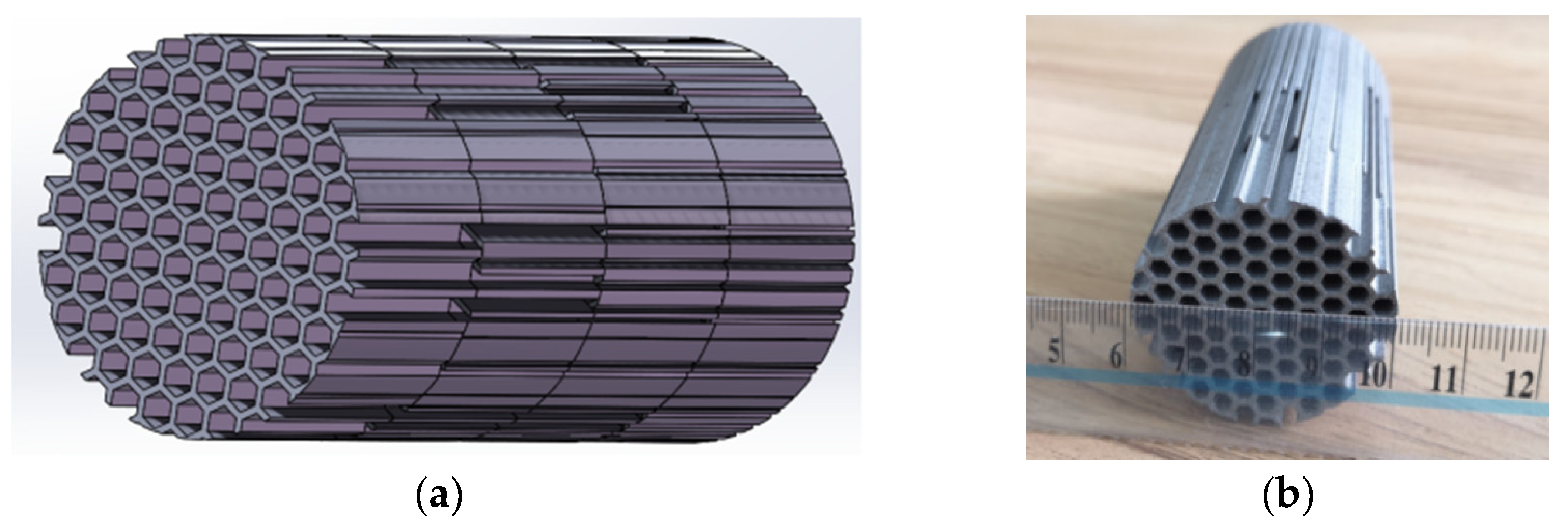
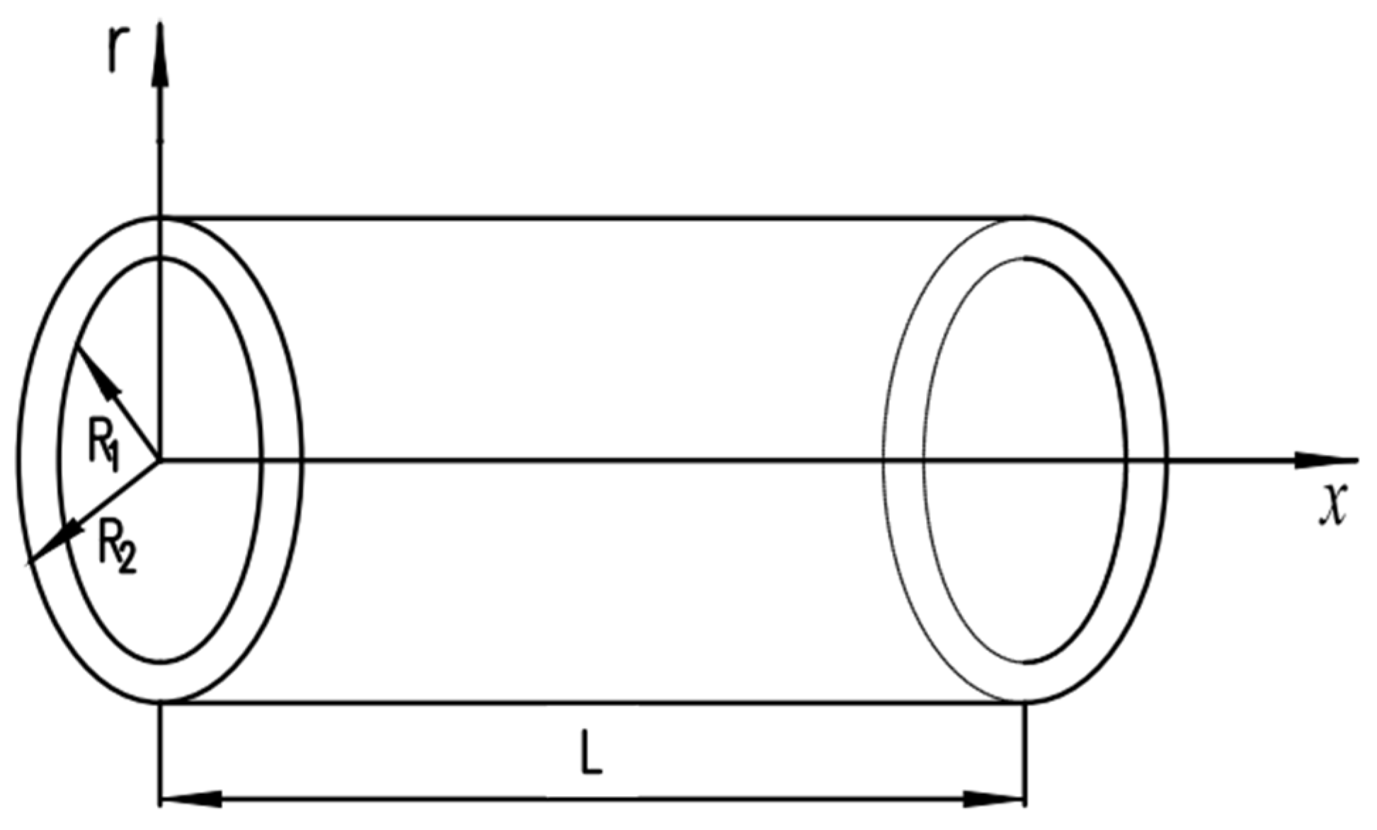
2.1. System Model and Regenerator Single-Tube Model

The complete process of the ideal Stirling cycle includes two working conditions: the isochoric process and the isothermal process, as Figure 2 illustrates.

In the figure, 1 → 2 and 3 → 4 represent the isothermal process conditions. The gas volume in the working chamber is compressed or expanded so that heat passes through the heat exchanger to achieve heating or cooling. Here, the heat exchanger works without a regenerator, which is characteristic of isothermal heat transfer.

In contrast, 2 → 3 and 4 → 1 signify isochoric process conditions. The volume of the working chamber remains unchanged during operation, and the gas travels back and forth within the regenerator, which absorbs or releases heat. Under these conditions, the regenerator works without the heat exchanger. Since the volume remains constant, the gas is regarded as incompressible.

In this paper, the axial heat conduction is ignored, so the research model is simplified as “radial heat transfer of an incompressible gas in a regenerator under oscillation”.

The system model is composed of phases 2 → 3 and 4 → 1 of the ideal Stirling cycle. Working with the regenerator, the system is composed of a piston, a regenerator, a chamber, etc., as Figure 3 shows.

The temperature distribution of the system is displayed in Figure 4. T_h, T_l, and T_r are the temperature of the hot chamber, the cold chamber, and the regenerator at the initial moment, and of T_h ± ΔT (Temperature of the hot chamber)_, T_l ± ΔT (Temperature of the cold chamber) and T_r + ΔT (Temperature of the regenerator)respectively, when working, so ΔT is the temperature change caused by oscillating flow, distributed linearly along the axial direction.

To develop a regenerator suitable for small temperature differences and low flow resistance, we designed a normal hexagonal bundle regenerator (see Figure 5a). The physical object was fabricated using additive manufacturing technology (see Figure 5b). We applied for a national invention patent for this regenerator and obtained authorization (authorization number: CN112944740B).

When the heat transfer area is equal to the volume-specific surface area, any single regular hexagonal tube in Figure 5 can be considered equivalent to a round tube, since the error of the analytical solution between a hexagonal tube and a circular tube is less than 2.3% 25. The equivalent single-tube physical model of the regenerator is shown in Figure 6, where R₁ is the limiting radius of the fluid and R₂ denotes the outer circle, while L is the length of the regenerator. Due to the symmetry of the hexagonal tube bundle honeycomb structure, the outer surface of the circular tube is set as the adiabatic surface.

2.2. Governing Equation

Assuming that the working medium in the system is an incompressible and fully developed fluid, the corresponding governing equation can be obtained according to the complex function theory [28].

The momentum conservation equation is:

$$\frac{\partial u}{\partial t}=-\frac{1}{\rho }\frac{\partial p}{\partial x}+\frac{\mu }{\rho }(\frac{{\partial }^{2}u}{\partial r^2}+\frac{1}{r}\frac{\partial u}{\partial r})$$

(1)

The boundary conditions satisfying Equation (1) are:

$$\left\{\begin{array}{c}r=R_1,u=0\\ r=0, \frac{\partial u}{\partial r}=0\end{array}\right.$$

Ignoring the viscous dissipation, the energy equation of the fluid is:

$$\frac{\partial T_f}{\partial t}+u(r,t)\frac{\partial T_f}{\partial x}={\alpha }_f(\frac{{\partial }^2{T}_f}{\partial r^2}+\frac{1}{r}\frac{\partial T_f}{\partial r}+\frac{{\partial }^2{T}_f}{\partial x^2})(0<r<R_1)$$

(2)

The energy equation of the solid is:

$$\frac{\partial T_w}{\partial t}={\alpha }_w(\frac{{\partial }^2{T}_w}{\partial r^2}+\frac{1}{r}\frac{\partial T_w}{\partial r}+\frac{{\partial }^2{T}_w}{\partial x^2})(R_1\le r\le R_2)$$

(3)

The boundary conditions satisfying Equations (2) and (3) are:

$$\left\{\begin{array}{c}r=0,\frac{\partial T_f}{\partial r}=0; (\mathrm{Center}-\mathrm{symmetric} \mathrm{temperature} \mathrm{distribution})\\ r=R_2,\frac{\partial T_w}{\partial r}=0; (\mathrm{The} \mathrm{outer} \mathrm{wall} \mathrm{of} \mathrm{the} \mathrm{tube} \mathrm{is} \mathrm{adiabatic})\\ r=R_1,T_f(R_1)=T_w(R_1), (\mathrm{Fluid} \mathrm{and} \mathrm{solid} \mathrm{temperatures} \mathrm{are} \mathrm{continuous} \mathrm{in} \mathrm{the} \mathrm{radial} \mathrm{surface} \mathrm{of} \mathrm{the} \mathrm{inner} \mathrm{wall})\\ \begin{array}{l}{\lambda }_f\frac{\partial T_f(R_1)}{\partial r}={\lambda }_w\frac{\partial T_w(R_1)}{\partial r} (\mathrm{Fluid} \mathrm{and} \mathrm{solid} \mathrm{heat} \mathrm{flow} \mathrm{are} \mathrm{continuous} \mathrm{in} \mathrm{the} \mathrm{radial} \mathrm{surface} \mathrm{of} \mathrm{the} \mathrm{inner} \mathrm{wall}) \\ \end{array}\end{array}\right.$$

3. Analysis of the Governing Equation

3.1. Pressure Fluctuation

Complex functions are equivalent to sine/cosine functions, which contain amplitude and phase information, and it is more convenient to deal with them mathematically. The midpoint coordinate of the simple harmonic motion of the piston is set as x₀, the piston amplitude is A_h, and the angular frequency is ω. Thus, the piston displacement x_h is:

$$x_h(t)=x_0-A_h{e}^{i\omega t}$$

(4)

Regarding the incompressible fluid, according to the law of conservation of mass, the average velocity of any section in a single round tube of the regenerator is constant. Therefore, the average velocity ${\overline{u}}_{in}$ of the fluid at a reference section in a single tube is:

$${\overline{u}}_{in}(t)=-i\omega A_{in}{e}^{i\omega t}$$

(5)

where A_in is the fluid amplitude. By solving A_in and substituting it into Equation (5), we obtain:

$${\overline{u}}_{in}(t)=-i\omega \frac{A_h}{N}{\left(\frac{R_h}{R_1}\right)}^2{e}^{i\omega t}$$

(6)

Here, N signifies the number of round tubes in the regenerator and R_h represents the piston radius.

By substituting Equation (6) into Equation (1), the pressure distribution of the fully developed flow inside the circular tube of a single regenerator is:

$$p(x,t)=p_m+\frac{1}{N}\rho {\omega }^2{A}_h{\left(\frac{R_h}{R_1}\right)}^2\left(\frac{L}{2}-x\right)e^{i\omega t}$$

(7)

where p_m—the average pressure, ρ—gas density, the pressure fluctuation p is related to the piston amplitude A_h, ω represents the angular frequency, and R_h is the piston radius.

The variable p_x is set as:

$$p_x=\frac{1}{N}\rho {\omega }^2{A}_h{\left(\frac{R_h}{R_1}\right)}^2$$

(8)

By taking the derivative of Equation (7) and substituting Equation (8) into it, we obtain:

$$\frac{\partial p}{\partial x}=-p_x{e}^{i\omega t}$$

(9)

3.2. Radial Flow Velocity of Fluid in the Pipe

Assuming the fluid velocity u has a complex solution:

$$u(r,t)=U(r)e^{i\omega t}$$

(10)

Solving U(r), and substituting Equation (7) into Equation (1), the radial oscillation velocity in the tube is obtained:

$$U(r)=i\frac{1}{N}\omega A_h{\left(\frac{R_h}{R_1}\right)}^2\left(\frac{J_0(r\sqrt{-i}{\beta }_{\nu })}{J_0(R_1\sqrt{-i}{\beta }_{\nu })}-1\right)$$

(11)

Here, ${\beta }_{\nu }$ represents the frequency parameter of the velocity, and is expressed as ${\beta }_{\nu }=\sqrt{\frac{\omega \rho }{\mu }}$. The difference between this equation and the previous velocity distribution function [29] is the expression of the pressure gradient p_x in Equation (11).

From Equations (10) and (11), the real solution of radial velocity can be expressed as (see Appendix A for the derivation process):

$$u_{real}(r,t)=\frac{1}{N}\omega A_h{\left(\frac{R_h}{R_1}\right)}^2\mathrm{Re}[i\left(\frac{J_0(r\sqrt{-i}{\beta }_{\nu })}{J_0(R_1\sqrt{-i}{\beta }_{\nu })}-1\right)e^{i\omega t}]$$

(12)

3.3. Fluid-Solid Coupling Radial Temperature

For our problem, we attempted a locally effective solution when the time mean axial temperature gradient in the regenerator tube had a constant γ value (γ = (T_h − T_l)/L). We also assumed that there was a complex functional temperature distribution in the fluid and tube wall with the following structure:

$$T_f(x,r,t)=\gamma \left(x+\frac{T_l}{\gamma }+R_1{g}_f(r)e^{i\omega t}\right)$$

(13)

$$T_w(x,r,t)=\gamma \left(x+\frac{T_l}{\gamma }+R_1{g}_w(r)e^{i\omega t}\right)$$

(14)

Note that for the regenerator, when x = 0, the initial temperature is T_l at the starting point of the regenerator, as Figure 4 indicates [12,30].

After deriving Equations (13) and (14), they can be substituted into Equations (2) and (3), respectively, to generate:

$$\frac{d^2{g}_f}{d{r}^2}+\frac{1}{r}\frac{d{g}_f}{dr}-i\frac{\omega }{{\alpha }_f}{g}_f=\frac{U(r)}{{\alpha }_f{R}_1} (0<r<R_1)$$

(15)

$$\frac{d^2{g}_w}{d{r}^2}+\frac{1}{r}\frac{d{g}_w}{dr}-i\frac{\omega }{{\alpha }_w}{g}_w=0 (R_1<r<R_2)$$

(16)

Equation (15) is an inhomogeneous Bessel equation whose solution is composed of a homogeneous general solution as well as an inhomogeneous solution:

$$g_f(r)=C_1{J}_0(r\sqrt{-i}{\beta }_f)+C_2{Y}_0(r\sqrt{-i}{\beta }_f)+g_s(r)$$

(17)

In Equation (17), ${\beta }_f$ is the frequency parameter of the temperature, and is determined by: ${\beta }_f=\sqrt{\frac{\omega }{{\alpha }_f}}$. The particular solution $g_s(r)$ satisfies:

$$g_s(r)={\delta }_1{J}_0(r\sqrt{-i}{\beta }_{\nu })+{\delta }_2$$

(18)

By substituting Equation (18) into Equation (15), we obtain:

$$-i{\delta }_1{J}_0(r\sqrt{-i}{\beta }_{\nu })({\beta }_{\nu }{}^2+{\beta }_f^2)-{\delta }_{2}i{\beta }_f^2=\frac{U(r)}{{\alpha }_f{R}_1}$$

(19)

Next, by substituting Equation (11) into Equation (19) and comparing the coefficients of both sides of the equation, we acquire:

$$g_s(r)=\frac{p_x}{{\omega }^2\rho R_1}(1-\frac{\omega }{{\alpha }_f({\beta }_{\nu }{}^2+{\beta }_f^2)}\frac{J_0(r\sqrt{-i}{\beta }_{\nu })}{J_0(R_1\sqrt{-i}{\beta }_{\nu })})$$

(20)

Similarly, Equation (16) is a homogeneous Bessel equation, and its solution is:

$$g_w(r)=C_3{J}_0(r\sqrt{-i}{\beta }_w)+C_4{Y}_0(r\sqrt{-i}{\beta }_w)$$

(21)

where ${\beta }_w$ represents the frequency parameter of the solid temperature: ${\beta }_w=\sqrt{\frac{\omega }{{\alpha }_w}}$.

The coefficients of C₁~C₄ in Equations (17) and (21) are calculated according to the boundary conditions. This was previously referred to as the center-symmetric temperature distribution, and the outside of the tube is adiabatic. Equations (17) and (21) are substituted into the boundary conditions to obtain four equations, and four variables C₁~C₄ are obtained by solving them.

$$\left\{\begin{array}{l}{C}_1=\frac{{(\frac{p_x}{{\omega }^2\rho R_1})}^2\frac{\omega {\beta }_{\nu }}{{\alpha }_f({\beta }_{\nu }{}^2+{\beta }_f^2)}\left(\frac{\omega }{{\alpha }_f({\beta }_{\nu }{}^2+{\beta }_f^2)}-1\right)\frac{J_1(R_1\sqrt{-i}{\beta }_v)}{J_0(R_1\sqrt{-i}{\beta }_{\nu })}}{{\beta }_f{J}_1(R_1\sqrt{-i}{\beta }_f)J_0(R_1\sqrt{-i}{\beta }_f)}\\ C_2=0\\ C_3=\frac{{\lambda }_f\frac{p_x}{{\omega }^2\rho R_1}\left(\frac{\omega \sqrt{-i}{\beta }_{\nu }}{{\alpha }_f({\beta }_{\nu }{}^2+{\beta }_f^2)}{J}_0(R_1\sqrt{-i}{\beta }_f)\frac{J_1(R_1\sqrt{-i}{\beta }_v)}{J_0(R_1\sqrt{-i}{\beta }_{\nu })}+\sqrt{-i}{\beta }_f\left(1-\frac{\omega }{{\alpha }_f({\beta }_{\nu }{}^2+{\beta }_f^2)}\right)J_1(R_1\sqrt{-i}{\beta }_f)\right)}{\left[\begin{array}{l}{J}_0(R_1\sqrt{-i}{\beta }_f){\lambda }_w{\beta }_w\left(\frac{J_1(R_2\sqrt{-i}{\beta }_w)}{Y_1(R_2\sqrt{-i}{\beta }_w)}{Y}_1(R_1\sqrt{-i}{\beta }_w)-J_1(R_1\sqrt{-i}{\beta }_w)\right)\\ +{\lambda }_f{\beta }_f{J}_1(R_1\sqrt{-i}{\beta }_f)\cdot \left(J_0(R_1\sqrt{-i}{\beta }_w)-\frac{J_1(R_2\sqrt{-i}{\beta }_w)}{Y_1(R_2\sqrt{-i}{\beta }_w)}{Y}_0(R_1\sqrt{-i}{\beta }_w)\right)\end{array}\right]}\\ C_4=-C_3\frac{J_1(R_2\sqrt{-i}{\beta }_w)}{Y_1(R_2\sqrt{-i}{\beta }_w)}\end{array}\right.$$

By substituting C₁~C₄ and the particular solution g_s(r) into Equations (17) and (21), the expressions of g_f (r) and g_w(r) can be obtained according to the boundary conditions (see Appendix B for the derivation process):

$$g_f(r)=\frac{{(\frac{p_x}{{\omega }^2\rho R_1})}^2\frac{\omega {\beta }_{\nu }}{{\alpha }_f({\beta }_{\nu }{}^2+{\beta }_f^2)}\left(\frac{\omega }{{\alpha }_f({\beta }_{\nu }{}^2+{\beta }_f^2)}-1\right)\frac{J_1(R_1\sqrt{-i}{\beta }_v)}{J_0(R_1\sqrt{-i}{\beta }_{\nu })}}{{\beta }_f{J}_1(R_1\sqrt{-i}{\beta }_f)J_0(R_1\sqrt{-i}{\beta }_f)}{J}_0(r\sqrt{-i}{\beta }_f)+\frac{p_x}{{\omega }^2\rho R_1}\left(1-\frac{\omega }{{\alpha }_f({\beta }_{\nu }{}^2+{\beta }_f^2)}\frac{J_0(r\sqrt{-i}{\beta }_{\nu })}{J_0(R_1\sqrt{-i}{\beta }_{\nu })}\right)$$

(22)

$$g_w(r)=\frac{{\lambda }_f\frac{p_x}{{\omega }^2\rho R_1}\left(\begin{array}{l}\frac{\omega \sqrt{-i}{\beta }_{\nu }}{{\alpha }_f({\beta }_{\nu }{}^2+{\beta }_f^2)}{J}_0(R_1\sqrt{-i}{\beta }_f)\frac{J_1(R_1\sqrt{-i}{\beta }_v)}{J_0(R_1\sqrt{-i}{\beta }_{\nu })}\\ +\sqrt{-i}{\beta }_f\left(1-\frac{\omega }{{\alpha }_f({\beta }_{\nu }{}^2+{\beta }_f^2)}\right)J_1(R_1\sqrt{-i}{\beta }_f)\end{array}\right)\left(J_0(r\sqrt{-i}{\beta }_w)-\frac{J_1(R_2\sqrt{-i}{\beta }_w)}{Y_1(R_2\sqrt{-i}{\beta }_w)}{Y}_0(r\sqrt{-i}{\beta }_w)\right)}{\left[\begin{array}{l}{J}_0(R_1\sqrt{-i}{\beta }_f){\lambda }_w{\beta }_w\left(\frac{J_1(R_2\sqrt{-i}{\beta }_w)}{Y_1(R_2\sqrt{-i}{\beta }_w)}{Y}_1(R_1\sqrt{-i}{\beta }_w)-J_1(R_1\sqrt{-i}{\beta }_w)\right)\\ +{\lambda }_f{\beta }_f{J}_1(R_1\sqrt{-i}{\beta }_f)\cdot \left(J_0(R_1\sqrt{-i}{\beta }_w)-\frac{J_1(R_2\sqrt{-i}{\beta }_w)}{Y_1(R_2\sqrt{-i}{\beta }_w)}{Y}_0(R_1\sqrt{-i}{\beta }_w)\right)\end{array}\right]}$$

(23)

Therefore, the real analytical solution of the radial temperature is:

$$T_{f\_real}(x,r,t)=\gamma x+T_l+\gamma R_1\mathrm{Re}[(C_1{J}_0(r\sqrt{-i}{\beta }_f)+g_s(r))e^{i\omega t}]$$

(24)

$$T_{w\_real}(x,r,t)=\gamma x+T_l+\gamma R_1\mathrm{Re}[C_3(J_0(r\sqrt{-i}{\beta }_w)-\frac{J_1(R_2\sqrt{-i}{\beta }_w)}{Y_1(R_2\sqrt{-i}{\beta }_w)}{Y}_0(r\sqrt{-i}{\beta }_w))e^{i\omega t}]$$

(25)

4. Analysis of Radial Heat Transfer Characteristics

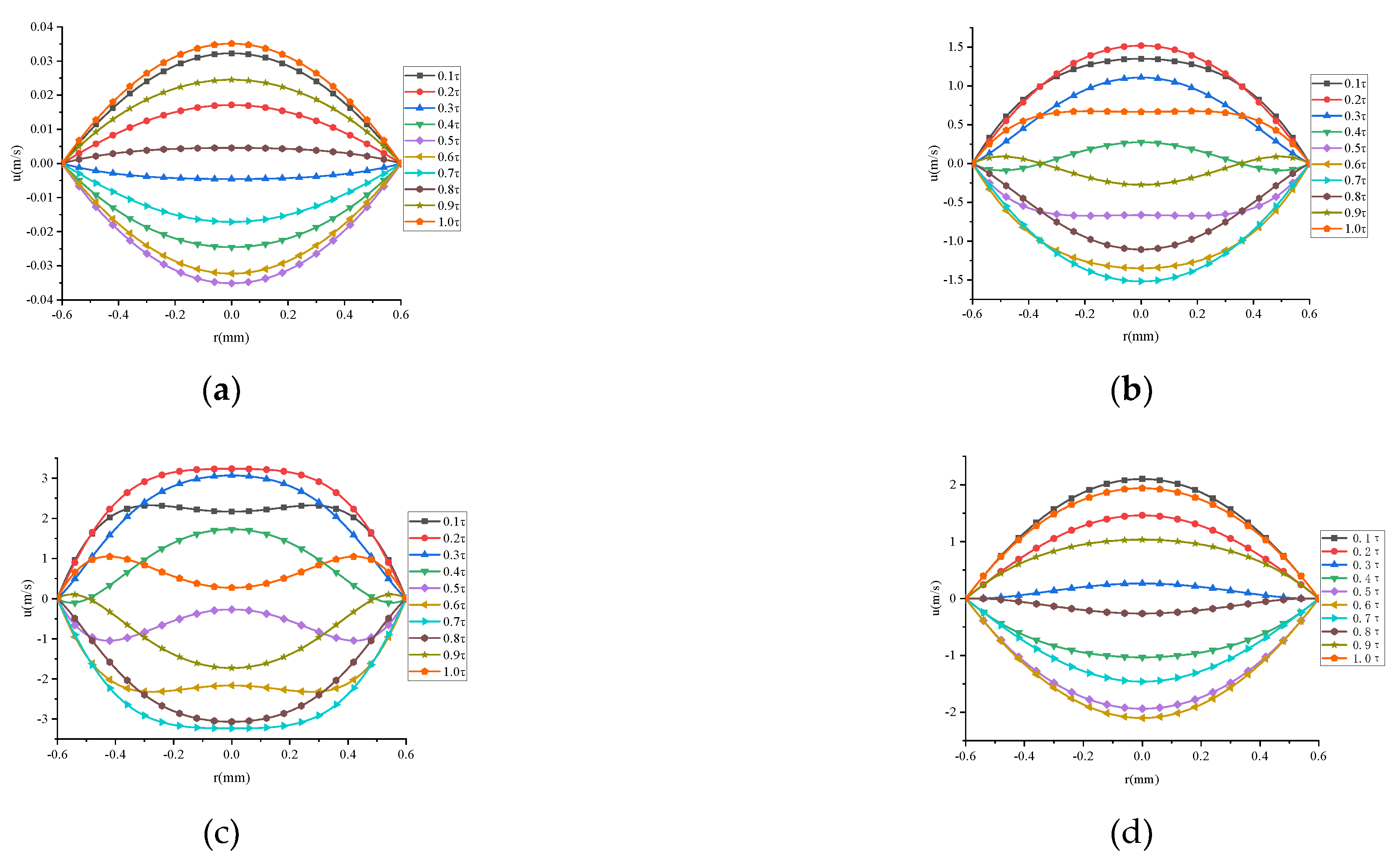
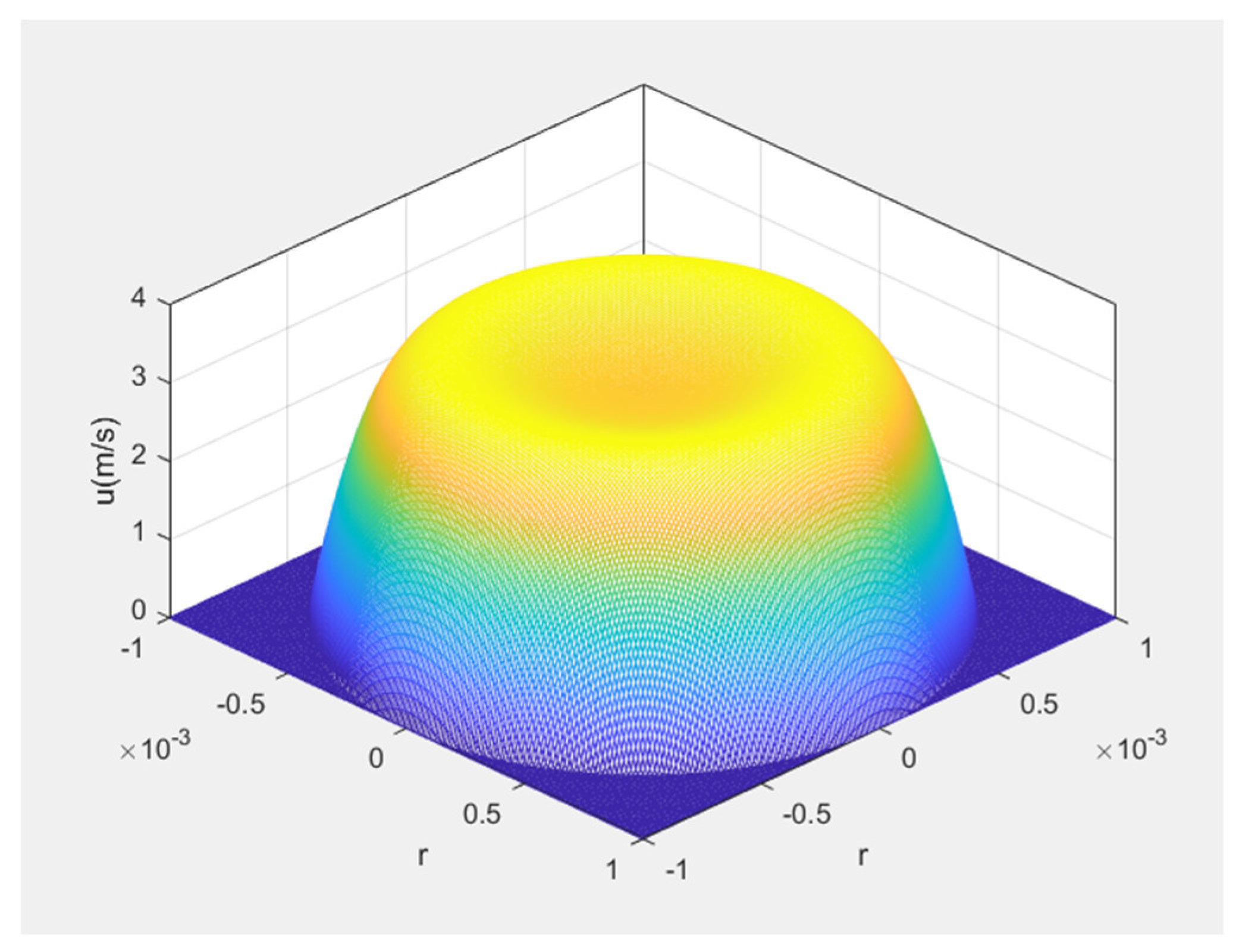
4.1. Radial Heat Transfer Characteristics of the Velocity Field

Aluminum alloy and carbon fiber are preliminarily selected as the regenerator materials, with air and helium as the fluids. The thermal and physical properties are outlined in

Table 1. Thermophysical properties of the regenerator tube wall (at 273 K).

Material	λw (W/m.K)	ρ (kg/m3)	Cp (W/m.K)	${\mathit{\alpha }}_{\mathit{w}}$ (m2/s)
AA (92Al-8Mg)	102	2610	904	4.32 × 10−5
CF	20	2000	700	1.43 × 10−5

and

Table 2. Thermophysical properties of the fluids (at 273 K, p = 1.01325 × 10⁵ Pa).

Fluid	λf (W/m.K)	ρ (kg/m3)	Cp (J/kg.K)	af (m2/s)	μ (Pa·s)	Cv (J/kg·K)
Air	24.07 × 10−3	1.293	1005	18.8 × 10−6	18.1 × 10−6	717
He	0.44	0.1785	5238	4.7 × 10−4	19.7 × 10−6	3213

[31]:

Additionally, we selected a piston radius of R_h = 20 mm, a piston amplitude of A_h = 6.5 mm, and an initial system pressure of p_m = 3 MPa.

Table 3. Initial parameters of the regenerator.

Parameter	R1 (mm)	R2 (mm)	L (mm)
Value	0.6	1	70

presents the initial design parameters of the regenerator [32].

When the oscillation frequency f is 6 Hz, 60 Hz, or 120 Hz, the radial velocity distribution curves of the fluid in a tube at various times within an oscillation cycle can be calculated according to Equation (12). The abscissa is the radius of the fluid tube, while the ordinate is the average radial velocity, as shown in Figure 7a–c. With a low frequency, the velocity is in a quasi-steady state and the velocity is similar to the Poiseuille distribution shown in Figure 7a. As the oscillation frequency increases, the velocity gradient becomes more concentrated in the area near the wall surface, exhibiting the so-called velocity loop effect, as Figure 7b shows. In addition, as Figure 7c reveals, this phenomenon is more obvious at higher oscillation frequencies. Since the viscosity coefficient of helium is much smaller, the velocity loop is only faintly visible when the frequency increases to 120 Hz, as Figure 7d shows.

In order to clearly display the velocity loop, a three-dimensional view is used. The three-dimensional graph shows the magnitude of the velocity u(longitudinal) in (r,θ). At some axial position x, u(r) is a function of r. According to Figure 8, the speed loop is low in the middle and high in the periphery. The initial conditions of the figure are consistent with those of Figure 7c.

It should be noted that at the position of r = 0, Equation (7) demonstrates that the maximum pressure fluctuation in the pipe is a quadratic function of the operating frequency. However, as Figure 9 reveals, relative to the average pressure of 3 MPa, the pressure fluctuation in the pipe does not exceed 0.017% of the average pressure, which is a small quantity of high order.

4.2. Heat Transfer Characteristics of the Fluid-Solid Coupling Surface

At the fluid-solid coupling surface, when r = R₁, the temperature of the fluid is equal to that of the solid. According to Equation (24), the temperature distribution of the fluid of its coupling surface is:

$$T_{f\_real}(x,R_1,t)=\gamma x+T_l+\gamma R_1\mathrm{Re}[(C_1{J}_0(R_1\sqrt{-i}{\beta }_f)+g_s(R_1))e^{i\omega t}]$$

(26)

Thus, the temperature amplitude ΔT is:

$$\Delta T=\gamma R_1\mathrm{Re}((C_1{J}_0(R_1\sqrt{-i}{\beta }_f)+g_s(R_1))$$

(27)

According to Equations (24) and (25), the temperature distribution at various times in the next oscillation cycle with different frequencies is shown in Figure 10a–c. When T_h = 330 K and T_l = 300 K, temperature loop of the fluid is visible.

Figure 10a–c reveal that although the thermal conductivity of the tube wall is much larger than the air, the temperature distribution of the air is obvious. With the increases in the frequency, the temperature amplitude rises as well. However, the tube wall is 2–3 orders of magnitude smaller than the air temperature amplitude, which is a straight line and cannot be observed. Therefore, it is necessary to enlarge the tube wall separately, as seen in Figure 10d, which shows the temperature distribution within a certain period. The temperature decreases regularly along the radius direction, indicating that the heat is transferred along the tube wall.

Figure 11 presents a three-dimensional view of the temperature distribution, which is similar to the velocity ring, since it is low in the middle and high at both ends, corresponding to Figure 10c.

The temperature distribution curves of the aluminum alloy and the carbon fiber within one cycle are displayed in Figure 12. The solid lines reflect the aluminum alloy while the dashed lines denote the carbon fiber. The figure reveals the temperature change along with the increase in wall thickness within one cycle. When the thermal diffusion coefficient is large, the heat conducts more quickly and the homogeneity of the temperature distribution is better; therefore, the change rate of the curve is relatively small.

According to Equation (27), at the fluid-solid coupling wall, the temperature amplitude changes with the frequency when different combinations of materials and working medium are present. Figure 13a,b illustrate how the wall temperature amplitude varies when the material remains unchanged and the working medium is changed. Since the thermal diffusivity of helium is much greater, the radial temperature is rapidly transmitted to the surface. Therefore, the temperature amplitude of helium under oscillation is much higher than that of air.

Additionally, as the frequency increases, the gap also grows. Figure 13c,d present the variation in the wall temperature when the working medium remains unchanged and the material is altered. Because the thermal conductivity of the aluminum alloy is much greater, it conducts heat more quickly, and the wall temperature amplitude of aluminum is much smaller than that of the carbon fiber.

Figure 13 shows the change in the temperature amplitude, which can be divided by frequency into three parts at the fluid-solid coupling wall: the unidirectional flow part, the low-frequency part, and the high-frequency part. When the frequency equals zero (f = 0), the wall temperature is a constant unidirectional flow part. Furthermore, the low-frequency part exists at 0 < f < f₀. When f > 0, the wall temperature begins to oscillate and the wall temperature’s amplitude is lower than it is during unidirectional flow. This is because, as the flow transforms from a unidirectional into an oscillating flow, the shear force in the fluid decreases with positive and negative changes in the flow direction. Accordingly, the temperature gradient and amplitude decrease at the same time. When f > f₀, further increasing the oscillation frequency leads to the appearance of a velocity loop, and the fluid shear force near the wall increases considerably. For helium, the shear force exceeds the value recorded during unidirectional flow. Due to the temperature loop, the gradient of the temperature rises with the increase in temperature amplitude. Moreover, f₀ appears at the lowest point of these curves.

The above analysis suggests that the minimum operating frequency of the system should avoid the low-frequency part. Additionally, Figure 13 demonstrates that the three parts of temperature amplitude against the frequency are greatly affected by the thermal diffusion coefficient of the gas. The low-frequency interval of helium is very narrow, and the wall temperature vibration value rises with the increase in frequency, as Figure 13b,d indicate.

Furthermore, we also assessed the relationship between temperature and frequency with different R₁ values and AA combinations. When R₁ varies between 0.5 mm and 2 mm, the full picture can be seen. Figure 14 indicates that at f = 80 Hz, the AA/air curve temperature amplitude crosses from the low-frequency into the high-frequency part.

4.3. Fluid-Solid Coupling Radial Heat Transfer Characteristics of the Heat Field

According to Equation (24), the radial temperature gradient of the fluid in the pipe is:

$$\frac{\partial T_{f\_real}}{\partial r}=\gamma R_1\mathrm{Re}[(\frac{p_x}{{\omega }^2\rho R_1}\frac{\omega \sqrt{-i}{\beta }_{\nu }}{{\alpha }_f({\beta }_{\nu }{}^2+{\beta }_f^2)}\frac{J_1(r\sqrt{-i}{\beta }_v)}{J_0(R_1\sqrt{-i}{\beta }_{\nu })}-C_1\sqrt{-i}{\beta }_f{J}_1(r\sqrt{-i}{\beta }_f))e^{i\omega t}]$$

(28)

Additionally, as in Equation (25), the radial temperature gradient of the pipe wall is:

$$\frac{\partial T_{w\_real}}{\partial r}=\gamma R_1\mathrm{Re}[(C_3\sqrt{-i}{\beta }_w(\frac{J_1(R_2\sqrt{-i}{\beta }_w)}{Y_1(R_2\sqrt{-i}{\beta }_w)}{Y}_1(r\sqrt{-i}{\beta }_w)-J_1(r\sqrt{-i}{\beta }_w)))e^{i\omega t}]$$

(29)

At r = R₁, either Equation (26) or Equation (27) can be used to obtain the radial temperature gradient as it varies with time within a period, as Figure 15 indicates.

In one cycle at r = R₁, the heat absorbed and the heat released are equal:

$${\left.Q(r)\right|}_{r=R_1}=\left\{\begin{array}{l}{\lambda }_{w}S\mathrm{Re}[{\displaystyle {\int }_{t_1}^{t_2}{\left.\frac{\partial T_w(r,t)}{\partial r}\right|}_{r=R_1}dt]}\\ {\lambda }_{f}S\mathrm{Re}[{\displaystyle {\int }_{t_1}^{t_2}{\left.\frac{\partial T_f(\mathrm{r},\mathrm{t})}{\partial r}\right|}_{r=R_1}dt}]\end{array}\right.$$

(30)

where S denotes the surface area of a single tube at the fluid-structure coupling of the regenerator. Also, S = 2πR₁L, satisfying t₁ = 0 and t₂ = π/ω.

At the wall surface, r = R₁, so the solid heat of a single tube in the regenerator is:

$$Q_{rw}(R_1)={\lambda }_{w}S\gamma R_1\mathrm{Re}[\frac{2C_3{\beta }_w}{\sqrt{-i}\omega }(J_1(R_1\sqrt{-i}{\beta }_w)-\frac{J_1(R_2\sqrt{-i}{\beta }_w)}{Y_1(R_2\sqrt{-i}{\beta }_w)}{Y}_1(R_1\sqrt{-i}{\beta }_w))]$$

(31)

The fluid heat for a single tube in the regenerator is:

$$Q_{rf}(R_1)={\lambda }_{f}S\gamma R_1\mathrm{Re}[\frac{2i\sqrt{-i}}{\omega }(\frac{p_x}{{\omega }^2\rho R_1}\frac{\omega {\beta }_{\nu }}{{\alpha }_f({\beta }_{\nu }{}^2+{\beta }_f^2)}\frac{J_1(R_1\sqrt{-i}{\beta }_v)}{J_0(R_1\sqrt{-i}{\beta }_{\nu })}-C_1{\beta }_f{J}_1(R_1\sqrt{-i}{\beta }_f))]$$

(32)

Furthermore, the radial distribution of heat flow at any point r in the wall of a single tube in the regenerator can be obtained, where R₁ < r < R₂.

$$Q_{rw}(r)={\lambda }_w\gamma s{R}_1\mathrm{Re}\left[\frac{2C_3{\beta }_w}{\sqrt{-i}\omega }\left(J_1(r\sqrt{-i}{\beta }_w)-\frac{J_1(R_2\sqrt{-i}{\beta }_w)}{Y_1(R_2\sqrt{-i}{\beta }_w)}{Y}_1(r\sqrt{-i}{\beta }_w)\right)\right]$$

(33)

In the same way, the radial distribution of heat flow at any point of a single tube in the regenerator can be obtained, where 0 < r < R₁.

$$Q_{rf}(r)={\lambda }_f\gamma s{R}_1\mathrm{Re}[\frac{2i\sqrt{-i}}{\omega }(\frac{p_x}{{\omega }^2\rho R_1}\frac{\omega {\beta }_{\nu }}{{\alpha }_f({\beta }_{\nu }{}^2+{\beta }_f^2)}\frac{J_1(r\sqrt{-i}{\beta }_v)}{J_0(R_1\sqrt{-i}{\beta }_{\nu })}-C_1{\beta }_f{J}_1(r\sqrt{-i}{\beta }_f))]$$

(34)

where s = 2πrL.

According to Equations (31)–(34), the heat distribution diagram can be plotted, and is shown in Figure 16. The figure presents a heat diagram for a single tube in the regenerator within a single cycle under different combinations of working medium and materials. The radial heat conduction is symmetrically distributed with r = 0 as the center. Since there is no heat exchange at the adiabatic boundary between r = 0 and r = R₂, Q(r) = Q(R₂) = 0. At the gas-solid coupling surface, when r = R₁, the heat reaches a maximum value, indicating that heat conduction mainly occurs at the wall surface. Figure 16a,c suggest that the heat Q(r) is lower at higher frequencies. When the frequency f ≥ 80 Hz in the fluid part (r < 0.4 mm), Q(r) < 0. This suggests that the heat transferred by the working medium in the interval described in Figure 15 is negative at this time. This is caused by the temperature loop effect and can be explained by Figure 11c.

For helium, the frequency has little effect on heat at the fluid-solid coupling surface, as Figure 16b,d indicate.

Figure 17 reveals how the heat varies at the fluid-solid coupling surface with different working medium. The figure shows that the influence of working medium causes significant differences. At a constant frequency, helium transmits more heat than air, and this advantage becomes more obvious at higher frequencies, as Figure 17a shows. Also, the difference in heat variation between air and helium is consistent with the analysis of temperature amplitude in Figure 13a. The AA/air heat curves differ greatly in the low-frequency part. However, as Figure 17b shows, when the frequency exceeds 30 Hz, the changes in heat are consistent. Moreover, R₁ has a considerable influence on the AA/He heat curve. Figure 17b reveals that, as R₁ increases, the heat of the fluid-solid coupling wall rises within a certain period.

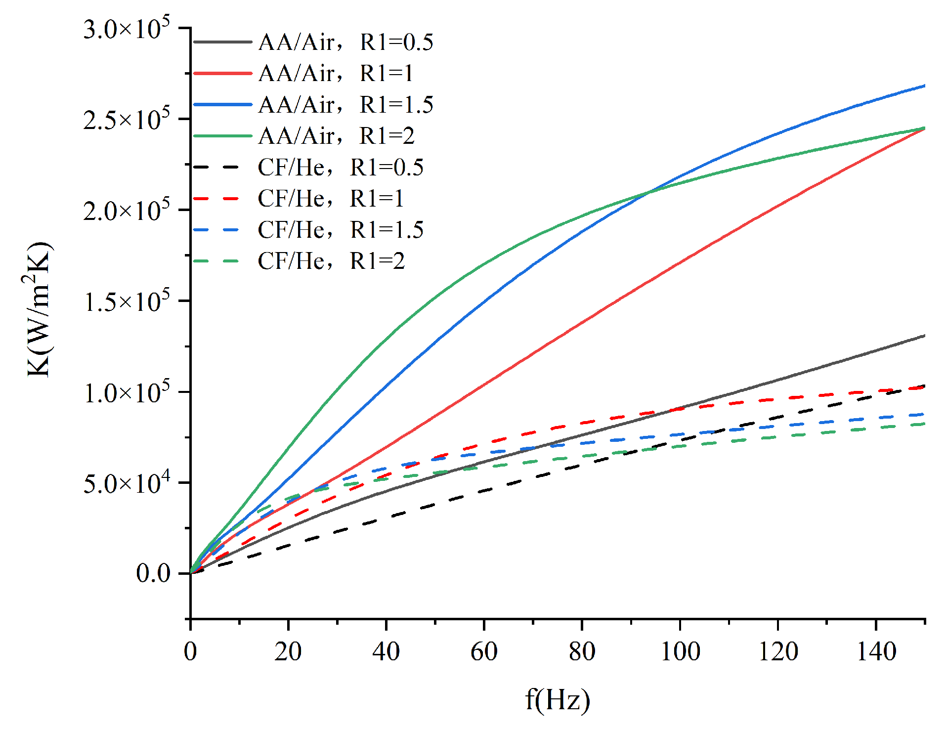
4.4. The EHTC under Oscillation

According to Equation (30), when r = R₁, the heat of the fluid is the same as that of the solid on the surface. Equation (31) expresses the fluid heat Q_rw(R₁) when r = R₁, where the heat transfer area S is related to diameter R₁ and length L; τ denotes the heat transfer time; and ΔT is the temperature amplitude, as shown in Equation (27). Thus, the EHTC K is:

$$K=\frac{Q_{rw}(R_1)}{\tau S\Delta T}=\frac{{\lambda }_w\mathrm{Re}[\frac{C_3{\beta }_w}{\sqrt{-i}\pi }(J_1(R_1\sqrt{-i}{\beta }_w)-\frac{J_1(R_2\sqrt{-i}{\beta }_w)}{Y_1(R_2\sqrt{-i}{\beta }_w)}{Y}_1(R_1\sqrt{-i}{\beta }_w))]}{\mathrm{Re}(C_1{J}_0(R_1\sqrt{-i}{\beta }_f)+g_s(R_1))}$$

(35)

Figure 18, which presents the K-f curves under different combinations of working medium and materials, indicates that the EHTC increases along with the rising frequency. Moreover, it is mainly dependent on the material, while it is less affected by the working medium.

According to Equation (36), the thermal conductivity λ_w of the material has a tremendous influence on the EHTC, because λ_AA > λ_CF; therefore, the EHTC of the aluminum alloy is greater than that of the carbon fiber. Using the same material, various combinations of working medium, such as AA/Air and AA/He, have different EHTC values. Additionally, the temperature amplitude ΔT in Equation (36) appears on the denominator, so its variations are the opposite of Equation (27). The frequency and the thermal diffusion coefficient of the fluid both influence the EHTC of the gas, as Figure 19 suggests.

5. Conclusions

The ideal Stirling cycle can be divided into two conditions, namely, the isochoric process and the isothermal process. The key to designing and optimizing the regenerator is to analyze the fluid-solid coupling radial heat transfer characteristics under isochoric process conditions.

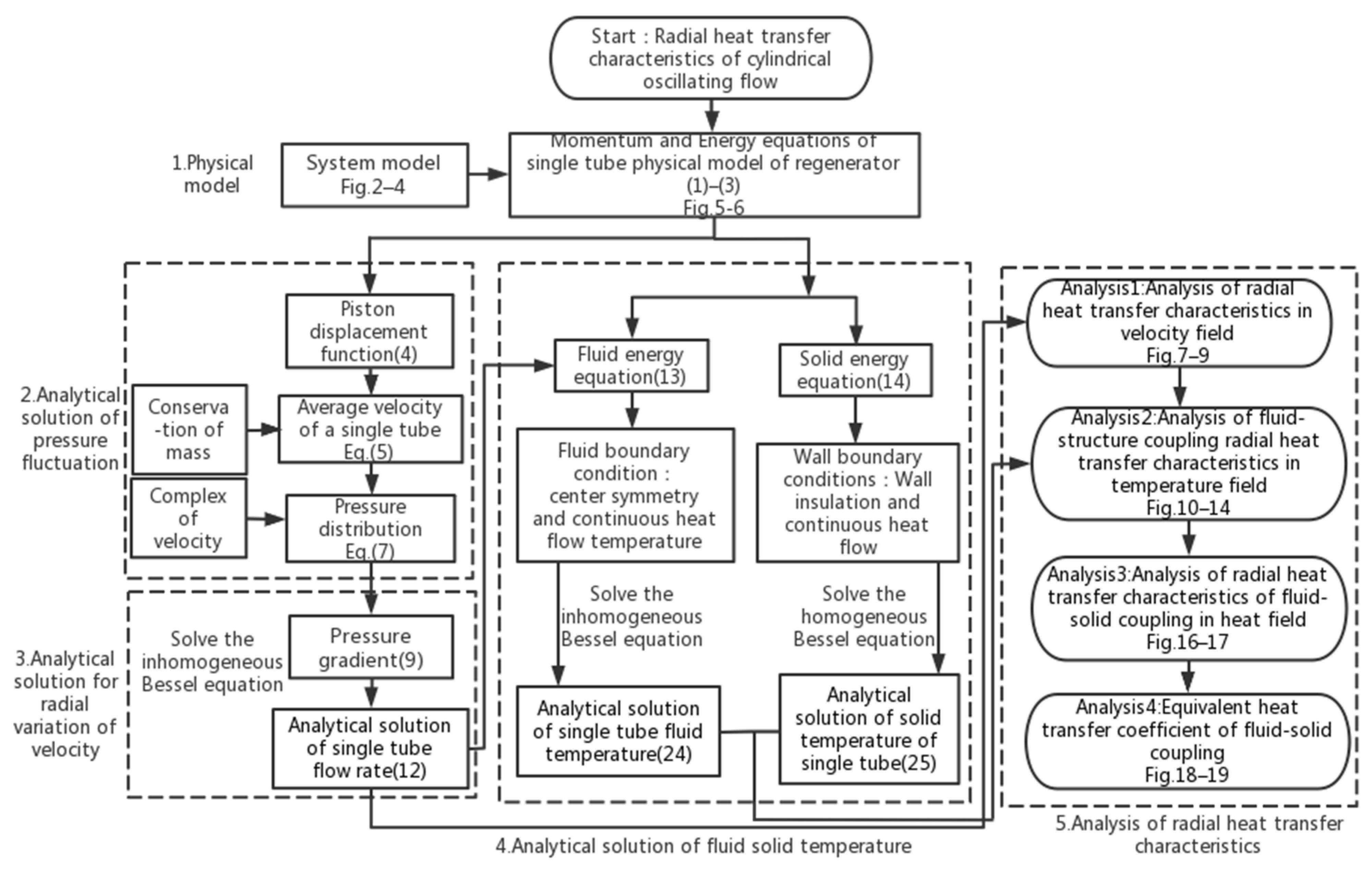
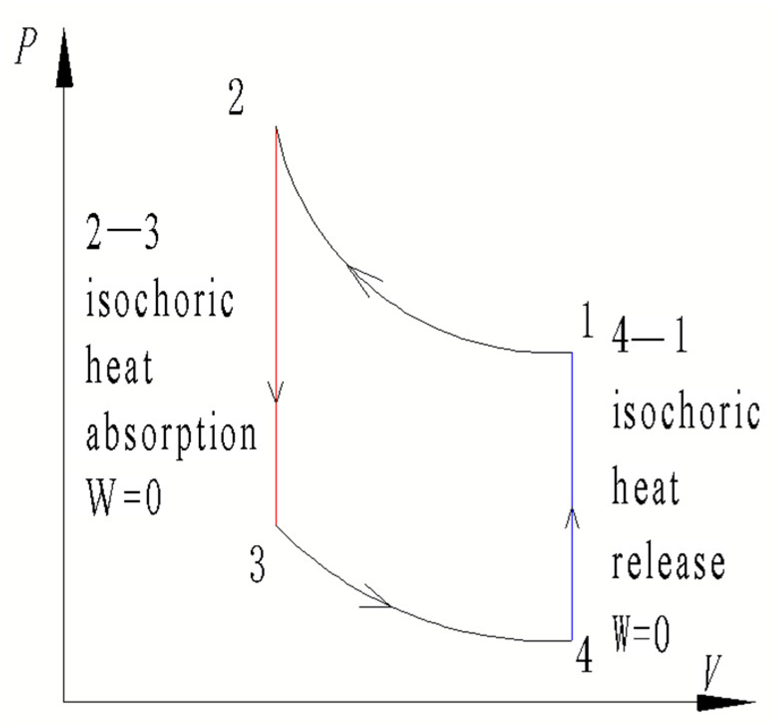
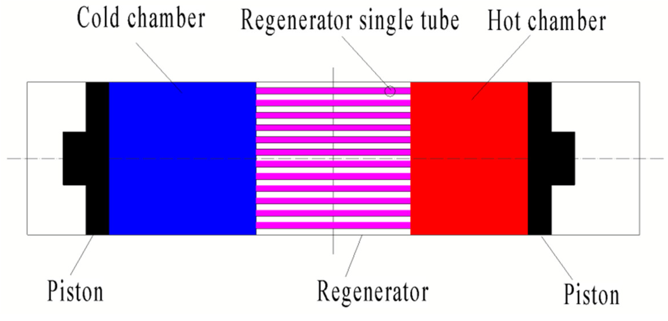
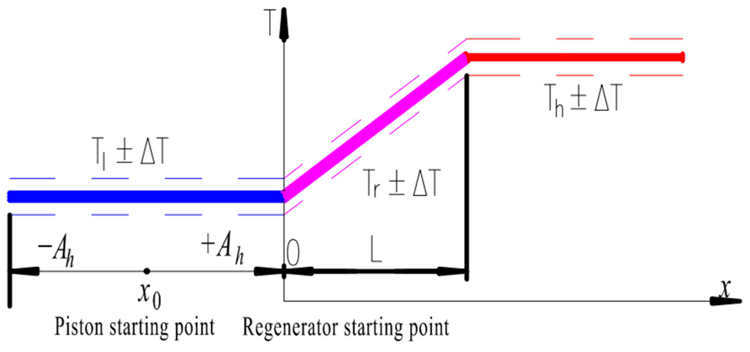
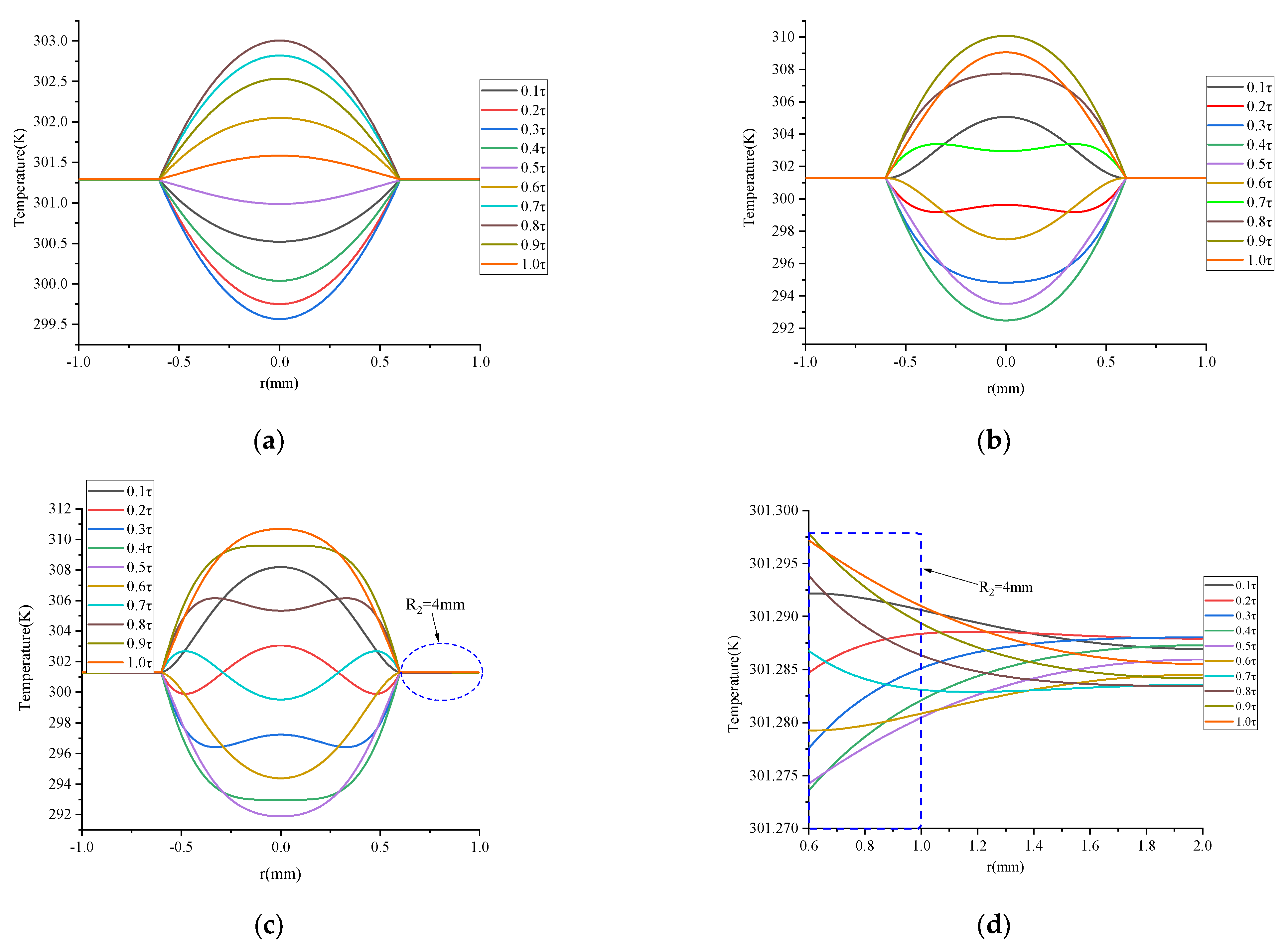
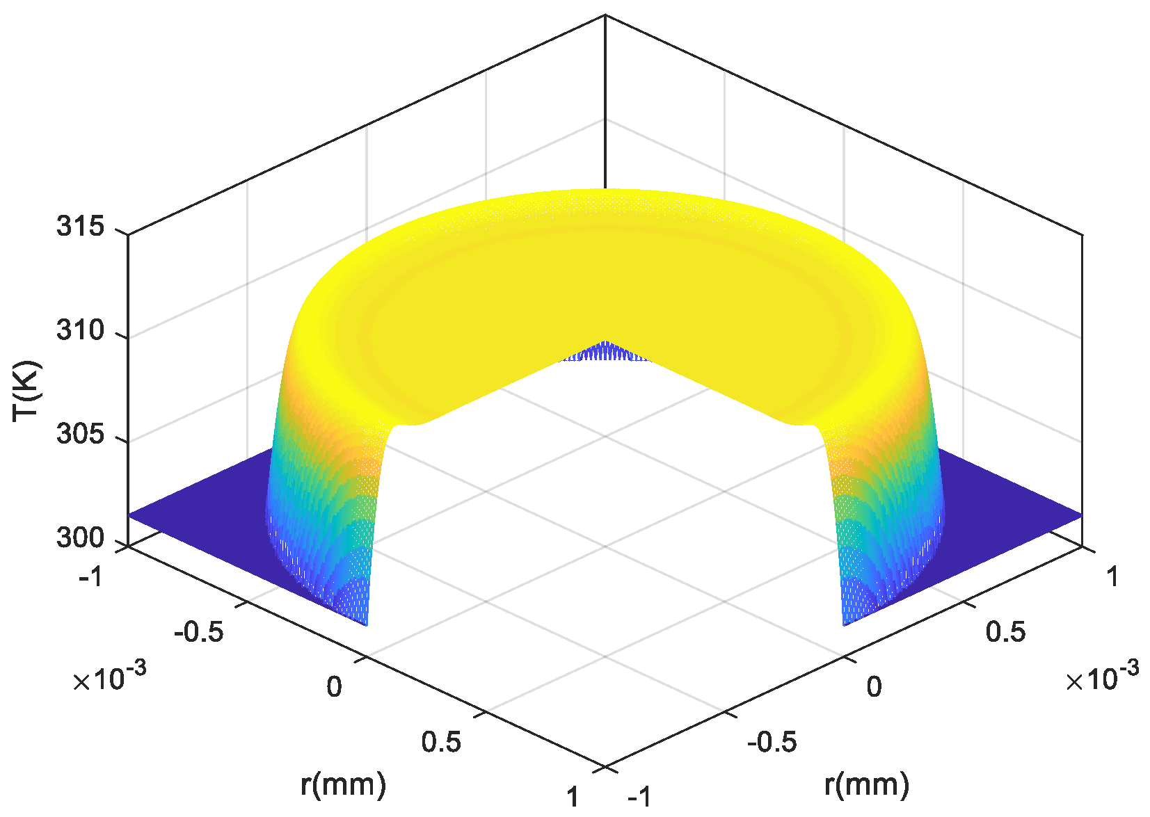
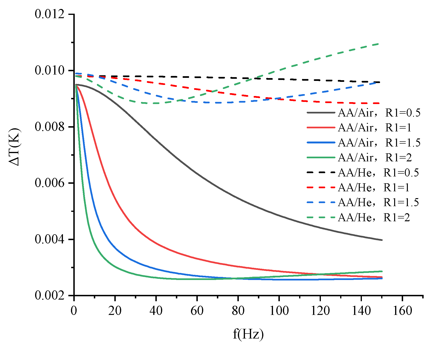
• By taking a normal hexagonal bundle regenerator as the object, we established a physical model of a closed system with an incompressible isochoric process under oscillating flow. The pressure fluctuation in the system was analyzed by associating piston motion with pressure fluctuation. In the complex domain, the fluid momentum equation and the energy equations were solved simultaneously. Also, the fluid velocity and the temperature distribution of the fluid-solid coupling wall were assessed. Finally, an analytical expression of radial heat transfer and the EHTC within a specified period were established. The analytical solutions of velocity, temperature, heat, and equivalent heat transfer coefficient were obtained, which revealed the following: Temperature amplitudes at different frequencies can be divided into three parts: the unidirectional flow part, with a constant wall temperature; the low-frequency part, where changes in temperature amplitude decrease dramatically under oscillation, which should be avoided when selecting the operating frequency; and the high-frequency part, in which the temperature amplitude gradually rises as the frequency increases.
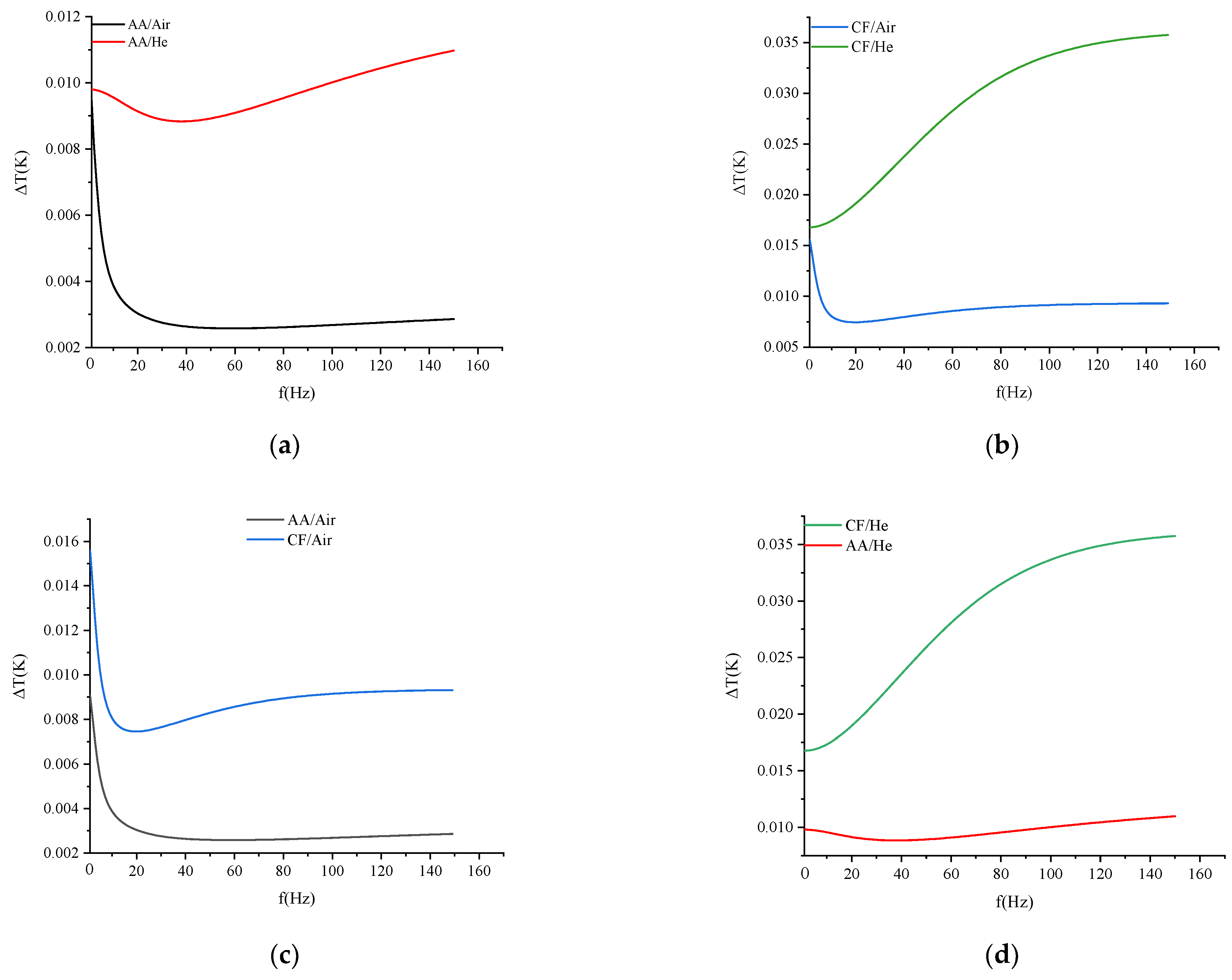
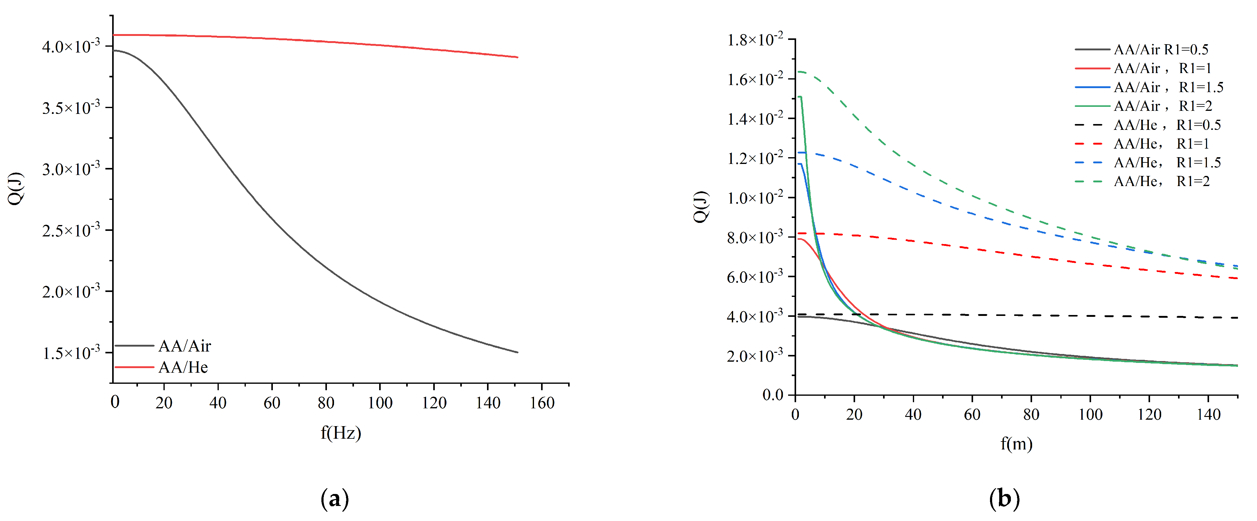
• Under the effect of frequency, the radial heat transfer of air and helium differs greatly in fluid-solid coupling. When air is the working medium, heat transfer drops sharply with increasing frequency in the low-frequency part. Subsequently, the decrease slows down until a certain point, where the amount of heat transferred remains roughly constant.
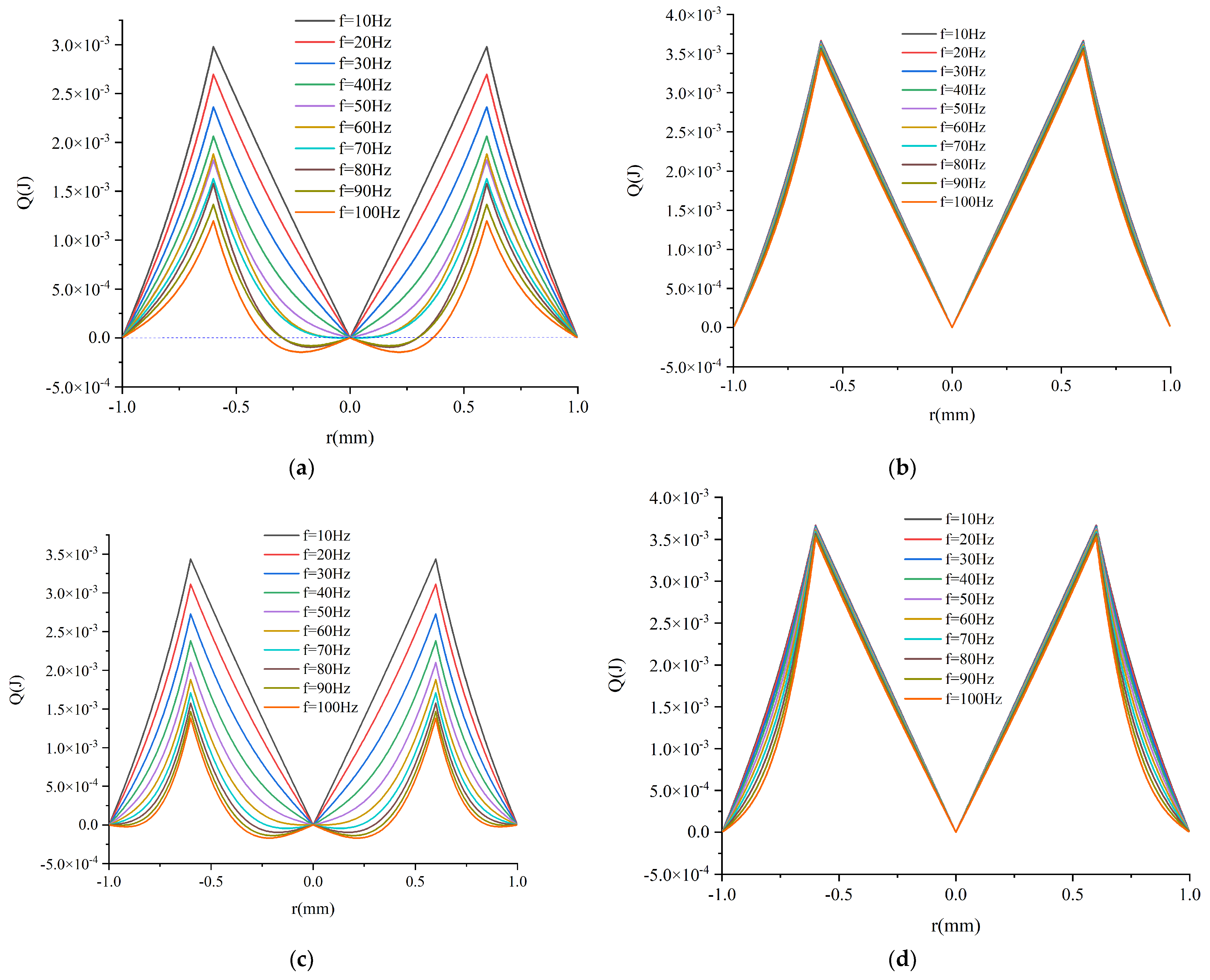
• When air is the working medium, its frequency is f ≥ 80 Hz, and the effect of the temperature loop means that heat transfer only occurs when r ≤ 0.4 mm. In this state, the fluid moves to the right.
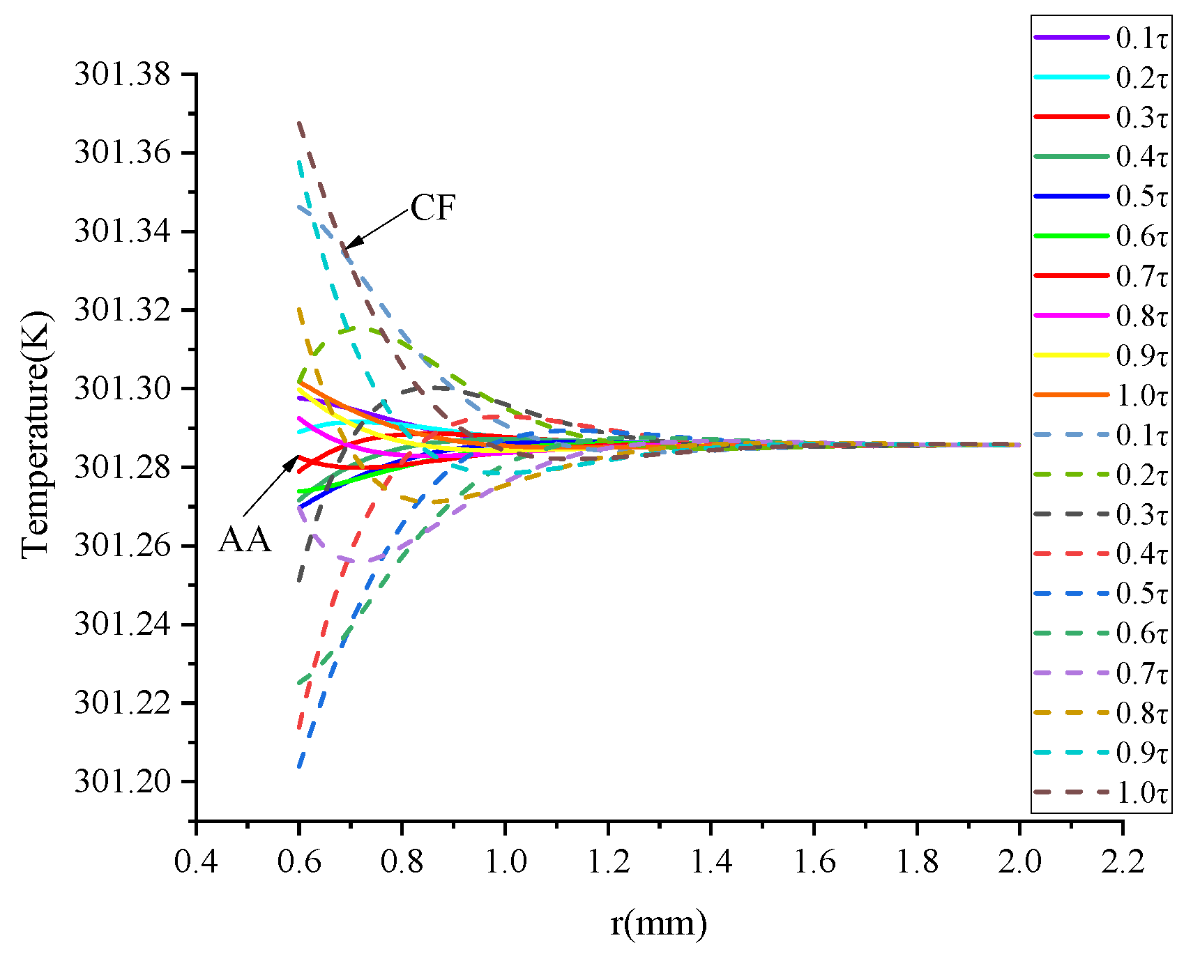
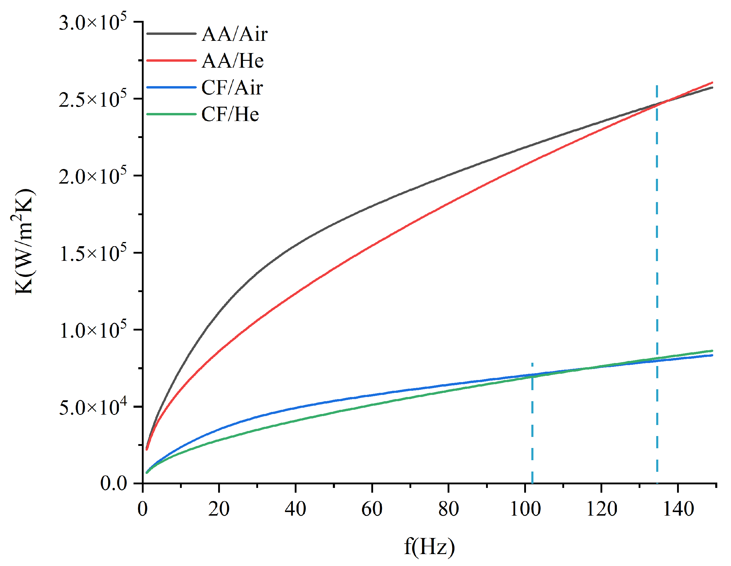
• The R₁ value that corresponds to the maximum heat value of the fluid-solid coupling surface is different from the R₁ that corresponds to the maximum EHTC. Thus, the value of R₁ can be considered as a compromise between fluid-solid heat coupling and the EHTC.

6. Patent

The following Chinese invention patent was produced: “Air Conditioning Temperature Zone Layered Honeycomb Structure with Variable Porosity Regenerator”, with the authorization number “ZL202110300042.7”.

References

1. Wang, Y.; Zhang, J.; Liu, B.; Dong, H.; Liu, X. Progress in Applications of Reverse Stirling Cycle Technology in Air Conditioning System of Pure Electric Vehicles. J. Xi’an Technol. Univ. 2021, 6, 609–620. [Google Scholar]
2. He, Y.-L.; Zhang, D.-W.; Yang, W.-W.; Gao, F. Numerical analysis on performance and contaminated failures of the miniature split Stirling cryocooler. Cryogenics 2014, 59, 12–22. [Google Scholar] [CrossRef]
3. Hachem, H.; Gheith, R.; Aloui, F.; Nasrallah, S.B.; Dincer, I. Exergy Assessment of Heat Transfer inside a Beta Type Stirling Engine. Int. J. Exergy 2016, 20, 186–202. [Google Scholar]
4. Hachem, H.; Gueith, R.; Aloui, F.; Dincer, I.; Ben Nasrallah, S. Energetic and Exergetic Performance Evaluations of an Experimental Beta Type Stirling Machine. In Progress in Clean Energy, Volume 2: Novel Systems and Applications; Springer: Berlin/Heidelberg, Germany, 2015; pp. 735–753. [Google Scholar]
5. Haywood, D.; Raine, J. Development of a Stirling-cycle Refrigerator. In IPENZ Conference 98; Informit: Wellington, New Zealand, 1998; pp. 40–44. [Google Scholar]
6. Haywood, D.; Raine, J.K.; Gschwendtner, M.A. Investigation of Seal Performance in a 4-α Double-Acting Stirling-Cycle Heat-Pump/Refrigerator. In Proceedings of the 10th International Stirling Engine Conference and Exhibition, Osnabrück, Germany, 20–25 May 2009; p. 132154. [Google Scholar]
7. Haywood, D.; Raine, J.K.; Gschwendtner, M.A. Stirling-cycle Heat-pumps and Refrigerators—A realistic alternative? In Proceedings of the Heating & Conditioning Engineers 2002 Conference, Christchurch, New Zealand; 2002; p. 4942-1. [Google Scholar]
8. Haywood, D. Investigation of Stirling-Type Heat-Pump and Refrigerator Systems Using Air as the Refrigerant. Ph.D. Thesis, University of Canterbury, Canterbury, UK, 2004. [Google Scholar]
9. Hachem, H.; Gheith, R.; Ben Nasrallah, S.; Aloui, F. Impact of Operating Parameters on Beta Type Regenerative Stirling Machine Performances. In Proceedings of the ASME-JSME-KSME 2015 Joint Fluids Engineering Conference, Seoul, Republic of Korea, 26–31 July 2015; p. 22088. [Google Scholar]
10. Hheith, H.; Gheith, R.; Nasrallah, S.B. Energetic and Exergetic Performance Evaluations of an Experimental Beta Type Stirling Machine; Springer International Publishing: Cham, Switzerland, 2015. [Google Scholar]
11. Nielsen, A.S.; York, B.T.; MacDonald, B.D. Stirling engine regenerators: How to attain over 95% regenerator effectiveness with sub-regenerators and thermal mass ratios. Appl. Energy 2019, 253, 113557. [Google Scholar] [CrossRef]
12. Wang, Y.; Zhang, J.; Zhang, T.; Lu, Z.; Dong, H. Analysis and Experiment of Heat Transfer Performance of Straight-Channel Grid Regenerator. Int. J. Heat Technol. 2022, 40, 781–791. [Google Scholar] [CrossRef]
13. Zhang, J.; Kurzweg, U. Numerical simulation of time-dependent heat transfer in oscillating pipe flow. J. Thermophys. Heat Transf. 1991, 5, 401–406. [Google Scholar] [CrossRef]
14. Zhao, T.; Cheng, P. A numerical solution of laminar forced convection in a heated pipe subjected to a reciprocating flow. Int. J. Heat Mass Transf. 1995, 38, 3011–3022. [Google Scholar] [CrossRef]
15. Zhao, T.; Cheng, P. The friction coefficient of a fully developed laminar reciprocating flow in a circular pipe. Int. J. Heat Fluid Flow 1996, 17, 167–172. [Google Scholar] [CrossRef]
16. Zhao, T.; Cheng, P. Oscillatory Heat Transfer in a Pipe Subjected to a Laminar Reciprocating Flow. J. Heat Transf. 1996, 118, 592–597. [Google Scholar] [CrossRef]
17. Zhao, T.; Cheng, P. Experimental studies on the onset of turbulence and frictional losses in an oscillatory turbulent pipe flow. Int. J. Heat Fluid Flow 1996, 17, 356–362. [Google Scholar] [CrossRef]
18. Jia, S.; Dong, J.Z.; Li, M.Z. A review on the flow characteristics of oscillating flow in Stirling engine. China Sci. Technol. Exp. 2011, 36, 387–389. [Google Scholar]
19. Brereton, G.J.; Jalil, S.M. Diffusive heat and mass transfer in oscillatory pipe flow. Phys. Fluids 2017, 29, 073601. [Google Scholar] [CrossRef]
20. Xiao, G.; Peng, H.; Fan, H.; Sultan, U.; Ni, M. Characteristics of steady and oscillating flows through regenerator. Int. J. Heat Mass Transf. 2017, 108, 309–321. [Google Scholar] [CrossRef]
21. Chen, Y.; Luo, E.; Dai, W. Heat transfer characteristics of oscillating flow regenerator filled with circular tubes or parallel plates. Cryogenics 2007, 47, 40–48. [Google Scholar] [CrossRef]
22. Zhao, L.; Zhu, G.; Cao, Y.; Zhu, D. Some problems of heat transfer enhancement by laminar viscous oscillating flow in capillary bundles. J. Beijing Univ. Aeronaut. Astronaut. 1991, 2, 57–66. [Google Scholar]
23. Wang, H.; Zhang, B.; Liu, M.; Rao, Z. Analytical solution of heat transfer performance of pin-array stack regenerator in stirling cycle. Int. J. Therm. Sci. 2021, 167, 107015. [Google Scholar] [CrossRef]
24. Wang, Y.; Zhang, J.; Lu, Z.; Liu, J.; Liu, B.; Dong, H. Analytical Solution of Heat Transfer Performance of Grid Regenerator in Inverse Stirling Cycle. Energies 2022, 15, 7024. [Google Scholar] [CrossRef]
25. Liu, X.; Jiang, Y.; Xia, J.; Chang, X. Analytical solutions of coupled heat and mass transfer processes in liquid desiccant air dehumidifier/regenerator. Energy Convers. Manag. 2007, 48, 2221–2232. [Google Scholar] [CrossRef]
26. Huang, J.; Shao, W.; Zhao, M.; Han, J.; Zhao, X.; Du, X.; Lv, X. Simplified Analytical Solution for Circular Tunnel under Obliquely Incident SV Wave. Soil Dyn. Earthq. Eng. 2021, 140, 106429. [Google Scholar] [CrossRef]
27. Liu, X.; Li, S.; Liu, L.; He, C.; Sun, Z.; Özdemir, F.; Aziz, M.; Kuo, P.-C. Research Progress on Convective Heat Transfer Characteristics of Supercritical Fluids in Curved Tube. Energies 2022, 15, 8358. [Google Scholar] [CrossRef]
28. Yang, Q.S.; Pu, B.R. Advanced Heat Transfer; Shanghai Jiaotong University Press: Shanghai, China, 2001; pp. 119–121. [Google Scholar]
29. Li, M.; Dong, J. Theoretical solution on heat transfer in oscillatory pipe flow and analysis of enhanced heat transfer. J. Aerosp. Power 2012, 27, 1967–1973. [Google Scholar]
30. Ma, D. Theory and nonlinearity of thermoacoustics. ACTA Acust. 1999, 4, 337–350. [Google Scholar]
31. Yang, S.; Tao, W. Heat Transfer; Higher Education Press: Beijing, China, 2006; p. 555. [Google Scholar]
32. Deng, W.; Li, Z.; Hu, J.; Xu, J.; Zhao, H. Design of the Stirling cryocooler with built-in pneumatic springs in displacer. Cryogenics 2021, 5, 8–11+27. [Google Scholar]
Figure 1. Logical flow chart.
Energies 16 06411 g001
Figure 2. P-V diagram in the ideal Stirling cycle.
Energies 16 06411 g002
Figure 3. Schematic diagram of the isochoric process.
Energies 16 06411 g003
Figure 4. Axial temperature distribution in the system.
Energies 16 06411 g004
Figure 5. Normal hexagonal bundle regenerator: (a) 3D model. (b) Physical object produced using 3D printing technology.
Energies 16 06411 g005
Figure 6. Equivalent single-tube physical model of the regenerator.
Energies 16 06411 g006
Figure 7. Effect of frequency and gas viscosity on velocity distribution (−0.6 mm ≤ r ≤ 0.6 mm) (a) f = 6 Hz, Air (b) f = 60 Hz, Air (c) f = 120 Hz, Air (d) f = 120 Hz, He.
Energies 16 06411 g007
Figure 8. Three−dimensional diagram of the velocity loop (f = 120, Air).
Energies 16 06411 g008
Figure 9. When x = 0, the pressure p in the tube is distributed with the frequency f.
Energies 16 06411 g009
Figure 10. Fluid-solid coupling temperature distribution of the regenerator (a) f = 6 Hz, Air/AA. (b) f = 60 Hz, Air/AA (c) f = 120 Hz, Air/AA (d) f = 120 Hz, Air/AA (R2 = 0.6 mm−2 mm).
Energies 16 06411 g010
Figure 11. Three−dimensional diagram of temperature distribution (f = 120 Hz, Air/AA).
Energies 16 06411 g011
Figure 12. Temperature distribution of the fluid-structure coupling wall in one period (f = 120 Hz).
Energies 16 06411 g012
Figure 13. ΔT-f curves for the fluid-solid coupling wall (ϕ = 0.64) (a) AA/Air vs. AA/He, (b) CF/Air vs. CF/He, (c) AA/Air vs. CF/Air, (d) AA/Air vs. CF/Air.
Energies 16 06411 g013
Figure 14. ΔT-f curves for the fluid-solid coupling wall at different R1 values (ϕ = 0.64).
Energies 16 06411 g014
Figure 15. Temperature gradient graph (f = 60 Hz).
Energies 16 06411 g015
Figure 16. Q-r curves under the influence of working medium and material: (a) AA/Air, (b) AA/He, (c) CF/Air, (d) CF/He.
Energies 16 06411 g016
Figure 17. Q-f curves at the fluid-solid coupling surface (ϕ = 0.64, R1= 0.5). (a) Q-f curves under different working conditions; (b) Q-f curves with different R1 values.
Energies 16 06411 g017
Figure 18. K-f curves under different working medium and material combinations (ϕ = 0.64).
Energies 16 06411 g018
Figure 19. K-f curves at different R1 values (ϕ = 0.64).
Energies 16 06411 g019