Water-Cut Measurement Techniques in Oil Production and Processing—A Review

Abstract

Water cut is a vital monitoring and surveillance parameter with great significance in oil production operations and processing. Water-cut measurements are also challenging due to the significant variations and the harsh measurement environment. The objective of this article is to review the current water-cut measurement techniques and suggest future areas that are expanding to overcome existing measurement challenges. Commercially available online methods such as capacitance-based sensors, tomography techniques, gamma densitometry, ultrasonic meters and infrared meters, and the traditional laboratory offline methods, are discussed, along with their principle of operation, detection range, and sensing resolution. Also, the discussed techniques are summarized, highlighting their main advantages and limitations. Furthermore, future trends and research areas, such as Artificial Intelligence (AI), soft computing, Metamaterials, and Nuclear Magnetic Resonance (NMR), which are integrated with water-cut measurements, are briefly mentioned. The current research hotspots are directed toward integrating full-range measurements with multi-parameter detection, high sensitivity, and reliability.

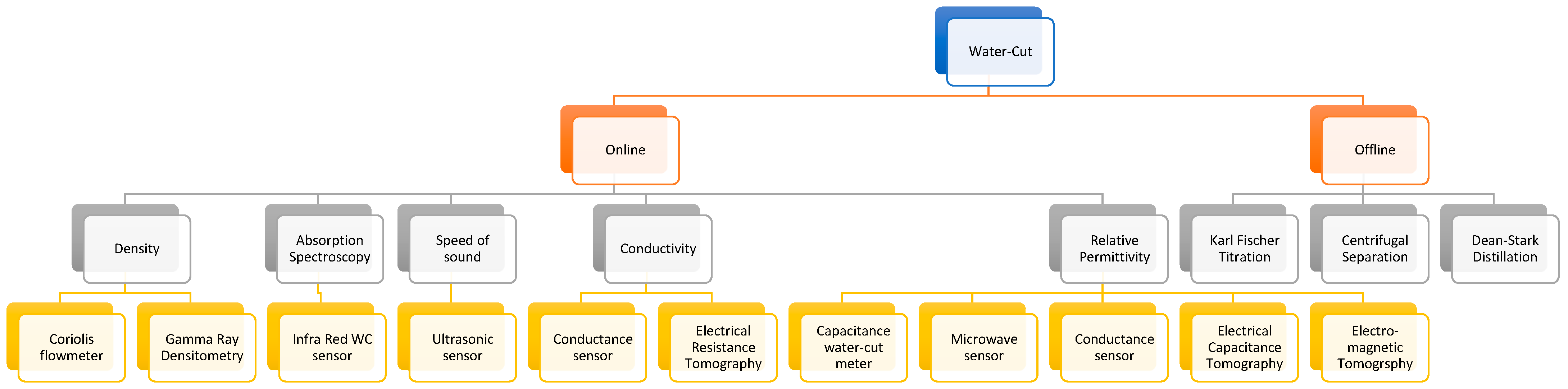
1. Introduction

The oil–water two-phase flow is commonly encountered in the exploration, development, and production of oil. In order to optimize the oil recovery, the accurate monitoring of the composition of the oil–water two-phase flow, particularly water cut, is critical [1]. The reliable determination of the fraction of water in the production stream, known as water-cut, is a critical production surveillance parameter. The main purpose of water-cut measurements is to determine the quality of the crude oil in the pipeline or flow lines, since minimal inaccuracies can lead to substantial revenue implications [2]. Water-cut measurements are vital for assuring the quality of the produced oil, marketing, custody transfer of crude oil, corrosion control, oil reservoirs’ material balance calculations, and minimizing bitumen loss to tailings in case of oil sands. A high water content can contaminate the produced oil and cause fouling and corrosion problems. Also, the separation of water is an energy-intensive process; thus, it is of paramount importance that the water content is correctly calculated and minimized, and that the economics of the produced crude oil are optimized. The high precision and stable online real-time water-cut detection is a key issue in surface production operations, the mining, processing, and transportation of crude oil, and its storage and marketing [1,2].

There are two primary methods for water-cut determination, including (1) online and (2) offline methods [3]. In offline production operations, the water cut is measured by taking a sample from the pipeline/flow line in the field and testing it in the laboratory for content analysis. Traditionally, methods like distillation, commonly known as Dean–Stark, Centrifuge, and Karl–Fischer titration, are used in the offline determination approach, where the measuring process may take up to a few days. Hence, they are highly time- and energy-consuming, limiting the number of samples available for analysis and, more importantly, delaying decisions that are to be made during operation, leading to a loss of production [3,4].

With the advent of technology, many different methods for water-cut measurements have appeared. Online methods, such as sensors based on infrared water-cut meters, Coriolis flow meters, and ultrasonic meters, can measure the water content accurately in real-time within a short period and reduce labor costs [4]. However, there are major disadvantages associated with online measurement techniques, such as sensitivity to temperature, salinity, corrosion, sulphur content, complex hydrocarbons, and limited water measurement range, that limit the real-life applicability of these methods.

In recent times, soft computing has gained attention as a potential tool for addressing engineering problems. This is attributed to the aptitude of soft computing in managing complex, dynamic, and non-linear issues, and its computational simplicity compared to analytical methods. It involves a range of techniques with the ability to manage imprecision and uncertainty, resulting in achievable solutions that are robust and economical [5].

In the context of multi-phase flow metering, soft computing approaches are employed to derive valuable information from traditional sensor outputs such as ultrasonic sensors, capacitance-based sensors, conductance sensors and Coriolis flowmeters. This information is then integrated with soft computing algorithms to make predictions or estimates of flow rates and phase fractions of multiphase flow, and identify different flow patterns [5].

Water and crude oil differ in terms of their physical properties such as density, permittivity, conductivity, and absorption spectroscopy. Many techniques developed based on the above-mentioned properties can be used to determine the water cut in multi-phase flows. Each technique comes with a different design approach, measurement range, accuracy, configuration, maintenance, and cost [6]. Figure 1 summarizes the most common water-cut measurement techniques. This review provides a basis for comparing various currently employed water-cut measurement techniques and their advantages and disadvantages.

Figure 1. Various water-cut measurement techniques.

2. Online Methods

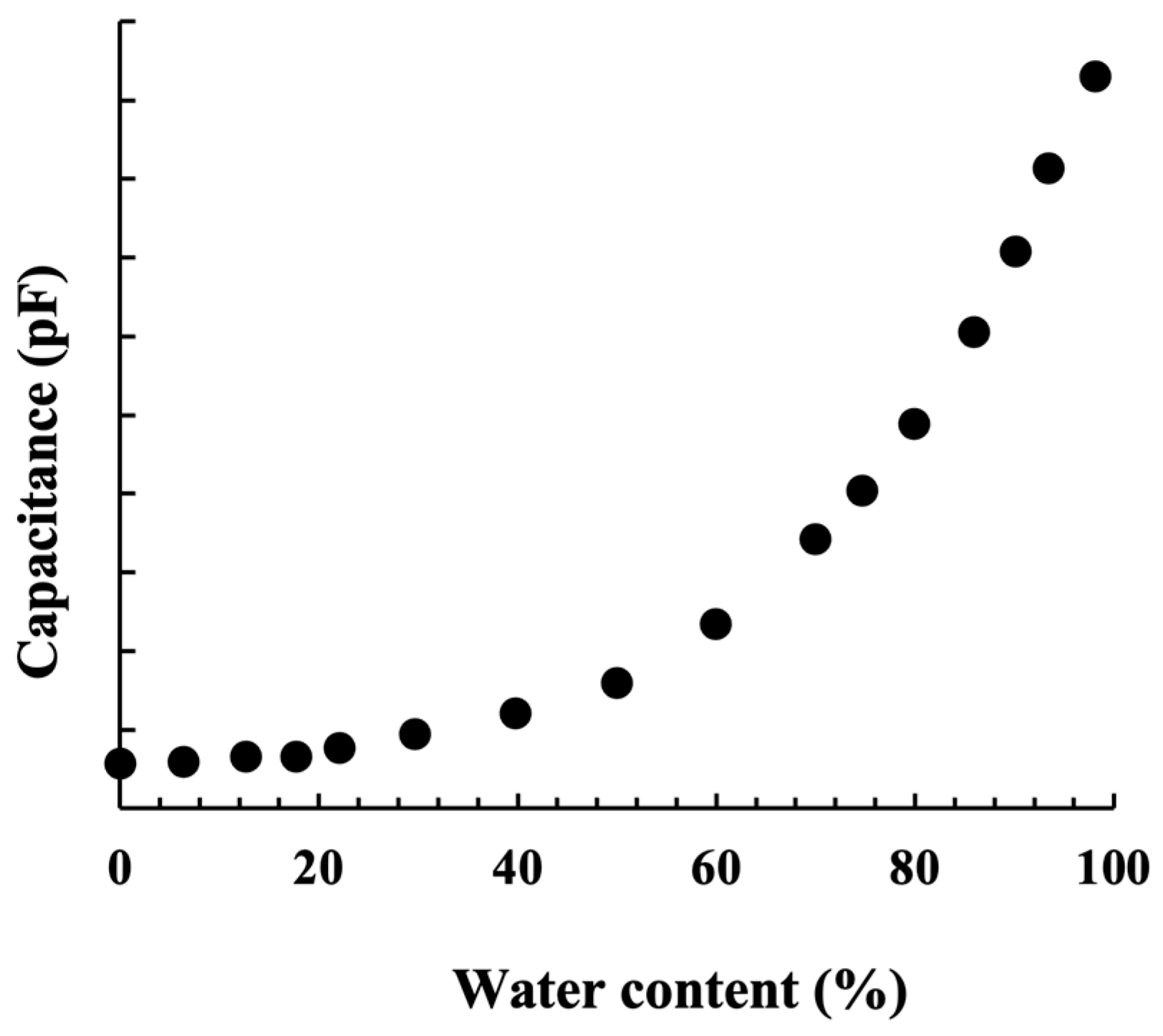
2.1. Capacitance-Based Water-Cut Meters

Capacitance-based water-cut meters rely on the dielectric properties of the water-in-oil emulsions and have been in use for more than 50 years [7]. They offer several advantages, such as a simple design and structure, being insensitive to water conductivity, a fast response speed, high sensitivity, and a low cost [6]. These sensors work best when the water cut is low and the continuous phase in the emulsion is oil (i.e., water droplets are dispersed in the oil phase). The relationship between water cut and the emulsion dielectric properties turns non-linear above ~10 vol.% of water [8]. As the water concentration of a water-in-oil emulsion increases (~35–60 vol.%), an inversion occurs, where the oil droplets are dispersed in water rather than the water dispersing in oil. At this point, as the emulsion becomes water-continuous, the conductivity of the capacitor increases, which limits the capacitance-based sensing analysis range to 50 vol.% water with light oil, and 80 vol.% with heavy oils [8].

While this method offers several advantages, some of the main drawbacks are as follows: (1) variations in the process parameters, such as density, temperature, and salinity, affect the capacitance value and, hence, the measured water cut; (2) entrained gas affects the net dielectric value of the fluid and decreases the measured value of the water cut [6]; (3) the capacitor sensor is subjected to contamination and wax deposition [9]; and hence requires regular maintenance; (4) in-line calibration is needed for reliable performance [6].

It is more commonly thought that the capacitive instruments can only function when a linear relation between water-cut and capacitance exists. However, it can extend through the non-linear region as well with the help of strapping tables [6]. Figure 2 shows the relationship between the data points of capacitance change with water cut [10].

Figure 2. Correlation of capacitance to water cut. Reproduced with permission from ref. [10].

Operating Principle: This technique relies on the large difference between the dielectric properties of oil and water. It takes advantage of the fact that the relative permittivity, ${\mathsf{\epsilon }}_{\mathrm{r}}$, of oil (${\mathsf{\epsilon }}_{\mathrm{r}}$: 2–3) is much smaller than that of water (${\mathsf{\epsilon }}_{\mathrm{r}}$: 80) [8]. The capacitance probe is composed of a stainless-steel cylindrical center rod coated with an insulated layer and a circular pipe as the main housing shield around it. The non-conductive, non-corrosive fluid flows in the annular space, giving rise to a dielectric medium. The dimensions of the probe are constant, and the capacitance value varies only with the change in the emulsion composition, which affects the dielectric constant. The relative permittivity of a sample under the test, ${\mathsf{\epsilon }}_{\mathrm{r}}$, is the ratio of the permittivity of that substance to the permittivity of the vacuum (i.e., ${\mathsf{\epsilon }}_{\mathrm{r}}=\mathsf{\epsilon }/{\mathsf{\epsilon }}_0$).

Usually, the measurement is made by applying a radio frequency (RF) signal between the probe and the pipe (outer electrode), which results in a minute current flow [7,11]. As shown in Equation (1), the change in the dielectric constant is directly proportional to the capacitance value due to the water cut, and hence can be converted to a water-cut output signal. The more water there is in the fluid medium, the higher the capacitance. The probe’s sensitivity can be improved by extending the probe length, $\mathrm{L}$, or decreasing the gap width.

Calculation of the capacitance of the sensor depends on the shape of the sensor. For a long cylindrical probe with a constant area, the capacitance is: [7]

$$\mathrm{C}=\frac{2\mathsf{\pi }\mathsf{\epsilon }\mathrm{L}}{\ln \left(\raisebox{1ex}{$\mathrm{b}$}\!\left/ \!\raisebox{-1ex}{$\mathrm{a}$}\right.\right)}$$

(1)

where a is the inner electrode radius, b is the outer electrode radius, $\mathsf{\epsilon }$(${\mathsf{\epsilon }}_{\mathrm{r}}{\mathsf{\epsilon }}_0$) is the permittivity of the dielectric medium gap, and $\mathrm{L}$ is the capacitor length.

The water-cut, as a function of dielectric constants of oil–water emulsion and individual constituents, is given by [7]:

$$\mathrm{W}\mathrm{C}=\frac{\left(\frac{{\mathsf{\epsilon }}_{\mathrm{r}\mathrm{o}}{\mathsf{\epsilon }}_{\mathrm{r}\mathrm{w}}}{{\mathsf{\epsilon }}_{\mathrm{r}\mathrm{w}}}\right)-{\mathsf{\epsilon }}_{\mathrm{r}\mathrm{w}}}{{\mathsf{\epsilon }}_{\mathrm{r}\mathrm{o}}-{\mathsf{\epsilon }}_{\mathrm{r}\mathrm{w}}}$$

(2)

where ${\mathsf{\epsilon }}_{\mathrm{r}}$ is the relative permittivity of a substance, and the subscripts $\mathrm{o}$, $\mathrm{w}$, $\mathrm{o}\mathrm{w}$ denote oil, water, and water-in-oil emulsion, respectively. A few other variations of the traditional capacitance meter have recently become more popular and are discussed below. Based on electrode configuration, capacitors can be broadly classified into invasive (direct contact between the electrode and fluid) and non-invasive (no contact between the metal electrode and liquid) [12].

Some of the most popular capacitance sensors for WC measurement are reviewed in the following section. Both no contact and in-contact sensing approaches are included.

2.1.1. Coaxial Capacitance Sensor (In-Contact)

The coaxial capacitance sensor is composed of a center electrode and an outer electrode, which is the metallic shell, as shown in Figure 3a. The center electrode is coated with an insulation layer, forming a capacitance with the outer electrode. The fluid flows between them and forms a capacitance with the outer electrode. When the oil–water emulsion flows past these electrodes, the capacitance value changes due to the different dielectric constants of oil and water, so the difference in the capacitance value indicates the change in the water cut. When the water cut value is high, the oil bubble size distribution and quantity in oil-in-water emulsions will influence the measured value of capacitance of the coaxial capacitance sensor [13].

Figure 3. (a) Structure of coaxial capacitance sensor. Reproduced with permission from ref. [13] and Copyright 2019 MDPI. (b) Schematic diagram of a wire-mesh sensor comprising a grid of electrodes [14]. Copyright 2013 Elsevier Ltd.

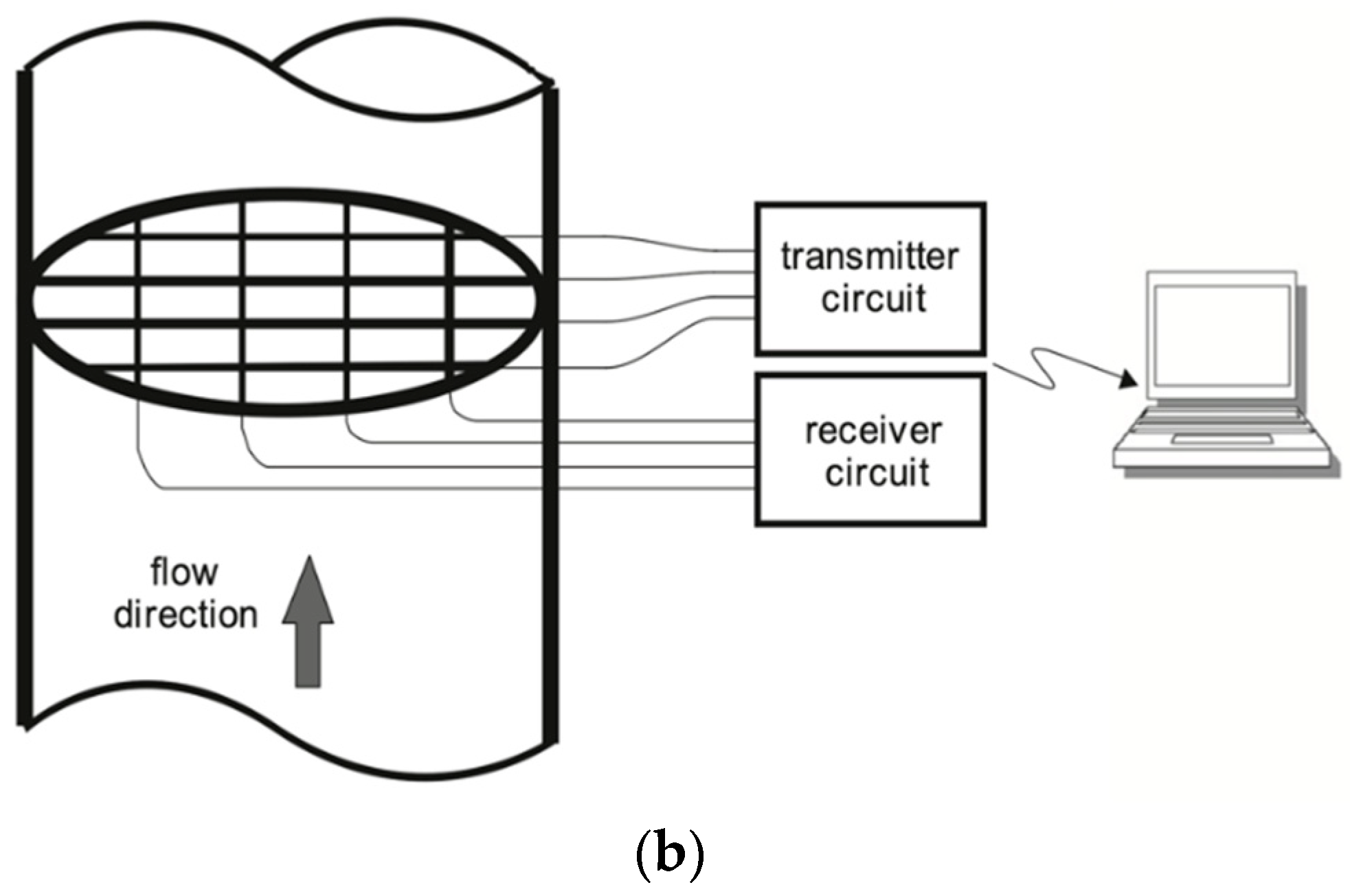
2.1.2. Capacitance Wire Mesh Sensor (In-Contact)

Capacitance wire-mesh sensors are intrusive, flow-imaging techniques that employ a high temporal resolution and spatial distribution to study multi-phase flow [14]. They consist of wire electrodes stretched over in two planes, which are 90° to each other, forming a network of electrodes, as shown in Figure 3b. The wires have a slight axial separation, typically of 2 mm. The system’s electronics can measure the electrical properties of the fluid in the confined spaces very quickly, thus generating images of phase distribution. The wire mesh sensor can measure the permittivity of the fluid at the crossing points. An AC voltage is applied to the transmitter wires, and the current flows to the receiver wires, which are arranged in parallel.

In this way, the sensor divides the regions into several sub-groups or sub-regions that independently determine the phase. These wire mesh sensors have been tested for air–water or water–oil flows. Recently, they have been tested for non-conducting fluids such as oil or organic liquids [14,15,16].

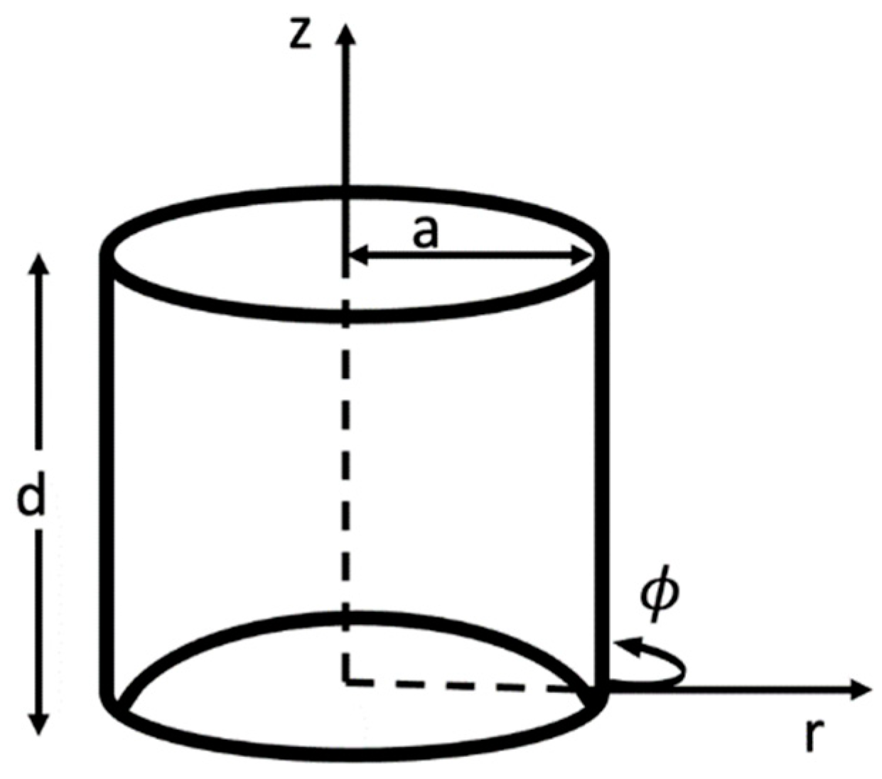
2.1.3. Principle of the Cylindrical Capacitance Sensor (Non-Contact)

The cylindrical capacitance sensor is made up of a metal shell (outer electrode), an outer insulating layer, a metal electrode, and an inner insulating layer [13]. The electrode and the insulating layer are very thin, at approximately 1 millimeter, as shown in Figure 4a. The metal shell is grounded, and the excitation voltage is given to the metal electrode, which insulates the metal shell. A cross-sectional view of the capacitance sensor is shown in Figure 4b [17]. The fluid flows throughout the length of the capacitor. In order to obtain a wider response strength for the fluid flowing through, it is necessary to have a wider runner so that the thickness of each layer is as small as possible. It is worth mentioning that the thinner the internal insulation layer, the more extensive the response range of the cylindrical capacitance sensor. These sensors work best when the oil–water emulsion is in a stratified state.

Figure 4. (a). Diagram of the cylindrical capacitance sensor. Reproduced with permission from ref. [13] and copyright 2019 MDPI. (b) Cross-sectional view of the cylindrical capacitance sensor. Reproduced with permission from ref. [17] and copyright 2002 IOP Publishing.

The metal casing and the inside insulating layer form a capacitance C₀, which can be determined by [17]

$${\mathrm{C}}_0=\frac{2\mathsf{\pi }{\mathsf{\epsilon }}_1{\mathsf{\epsilon }}_0\mathrm{L}}{\ln \left({\mathrm{R}}_3/{\mathrm{R}}_2\right)}$$

(3)

where ${\mathrm{R}}_0$ is the emulsion flow radius, ${\mathrm{R}}_1$ is the inside insulation layer radius, ${\mathrm{R}}_2$ is the electrode layer radius, ${\mathrm{R}}_3$ is the outside insulation layer radius, ${\mathsf{\epsilon }}_0$ is the relative permittivity of the electrode layer, ${\mathsf{\epsilon }}_1$ is the relative permittivity of the outside insulation layer and $\mathrm{L}$ is length of the sensor, as shown in Figure 4b. The water present at the base of the sensor can be considered a grounded electrode since water is a good conductor of electricity at a low frequency. The surface of the water can be divided into two sections, including S₁, the surface of the water in contact with the sensor wall and S₂, the interface of the oil–water emulsion. The electrode layer, the inside insulation layer and the water surface in contact with the insulating layer, S₁, form another capacitance, namely, ${\mathrm{C}}_1$. The S₁ layer is variable as it increases with the increase in the angle $\mathsf{\alpha }$ and the water hold-up, H. The value of capacitance ${\mathrm{C}}_1$ is calculated as [17]

$${\mathrm{C}}_1=\frac{\mathsf{\alpha }{\mathsf{\epsilon }}_1{\mathsf{\epsilon }}_0\mathrm{L}}{\ln \left(\raisebox{1ex}{${\mathrm{R}}_1$}\!\left/ \!\raisebox{-1ex}{${\mathrm{R}}_0$}\right.\right)}$$

(4)

Lastly, the electrode layer, the inside insulating layer and the water–oil surface in contact with the insulating layer, S₂, form another capacitance ${\mathrm{C}}_2$. The measured value of capacitance ${\mathrm{C}}_2$ is small, contributes very little, and can be neglected for simplicity [17]. The total capacitance can be obtained when the individual capacitances are connected in parallel and is given by [17]:

$$\mathrm{C}=\frac{2\mathsf{\pi }{\mathsf{\epsilon }}_1{\mathsf{\epsilon }}_0\mathrm{L}}{\ln \left({\mathrm{R}}_3/{\mathrm{R}}_2\right)}+\frac{\mathsf{\alpha }{\mathsf{\epsilon }}_1{\mathsf{\epsilon }}_0\mathrm{L}}{\ln \left({\mathrm{R}}_1/{\mathrm{R}}_0\right)}$$

(5)

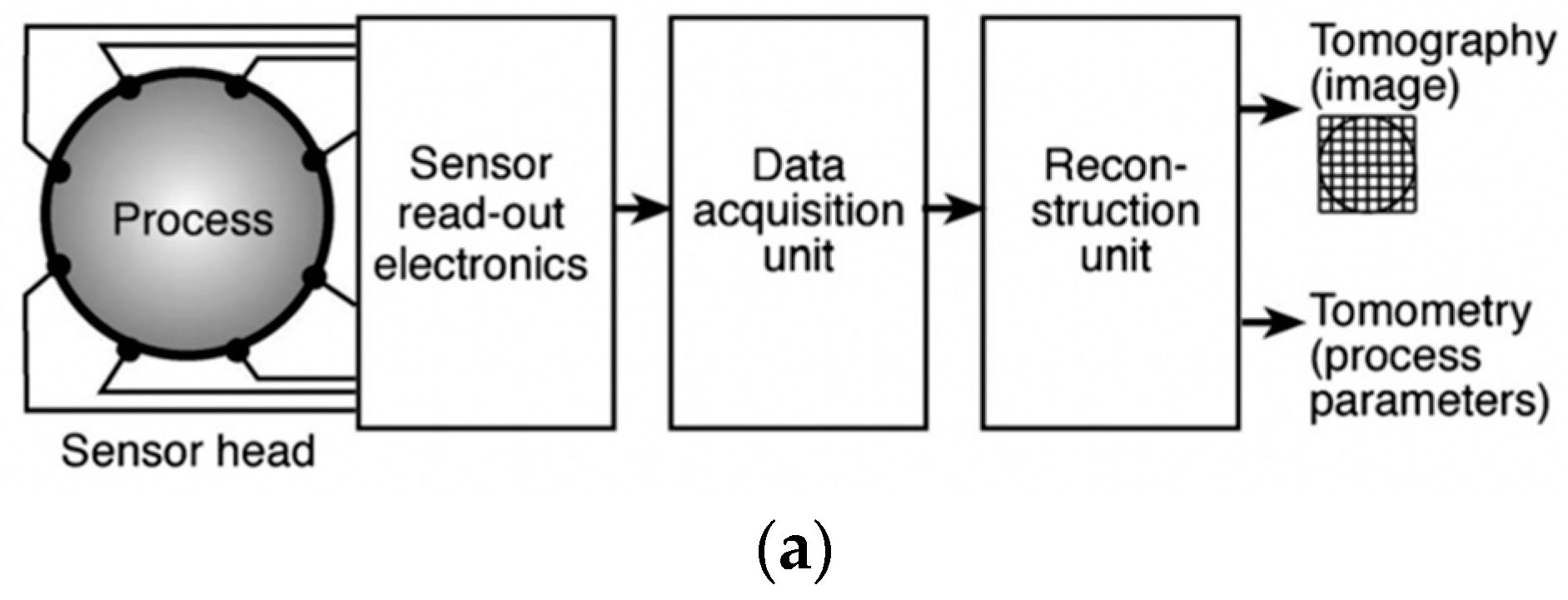
2.2. Tomography-Based Water-Cut Meters

The word “tomography” stems from the Greek ‘tomos’, meaning ‘slice’ and ‘graph’ meaning ‘image’. Tomography-based water-cut meters are non-intrusive techniques designed to generate a 2-D image of the cross-section of the vessel/object being measured in the industrial processes [18]. These methods provide useful information that can be used for the monitoring, visualization and verification of a mathematical model [19]. They have two major advantages over other measurement techniques. First, the measurements are non-invasive (i.e., they do not interfere with the measured object) and, second, the property of interest is measured many times within the same plane. The option to choose a given tomographic technique depends on the physical property of the fluid being measured and the temporal and spatial resolution [18]. The results obtained from a tomography method can be either an image (tomography), or process parameters, or properties that describe the distribution of the component in the process (tomometry), as shown in Figure 5a [20]. There are many types of tomography technique, such as Electrical Capacitance Tomography (ECT), Electrical Resistance Tomography (ERT), Electromagnetic Tomography (EMT), Gamma Ray Tomography and X-ray Tomography.

Figure 5. (a) General schematic diagram of a tomography system. The output of the tomography method is either an image (tomography) or a set of process parameters (tomometry) [20]. Copyright 2013 IOP Publishing Ltd. (b) Electrical Tomographic System [21]. Copyright 2001 SPIE and IS & T.

A typical electrical tomography system consists of sensors, electronics, switching electronics, signal conditioning, analogue/digital conversion, communications and a computer hosting control and data processing, including inversion, analysis and display algorithms, as shown in Figure 5b. A ring of electrodes is arranged in the region to be investigated. For capacitance and inductance tomography systems, the electrodes are usually non-invasive and non-intrusive. The non-invasive electrodes are not in direct contact with the flowing medium, and the non-intrusive electrodes do not obstruct the flow channel by extending into the process vessel. However, the electrodes are usually non-intrusive and invasive in electrical resistance tomography systems [21].

Some of the basic features and underlying principles of the tomography techniques are discussed below.

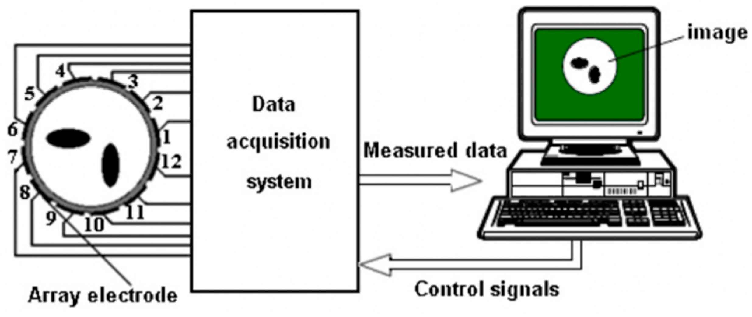
2.2.1. Electrical Capacitance Tomography (ECT)

Electrical Capacitance Tomography (ECT) is a non-intrusive, fast data-acquiring, non-radiating and non-hazardous technique [19]. The electrodes are usually present outside the vessel and are mounted on the periphery of the flow pipe. They measure the change in the value of capacitance due to the change in the permittivity of the components present in the fluid, as shown in Figure 6. ECT is composed of the forward and inverse problem. The forward problem is to find the capacitance value, while the inverse problem is the image reconstruction [22]. This is usually achieved using the Linear Back Projection (LBP) method [23].

Figure 6. An ECT system with a 12-electrode sensor [22]. Copyright 2009 IOP Publishing Ltd.

ECT is a “soft-field technique”, as the path of the transmitting signal is affected by the presence of dielectric and conductive materials, which can distort the electric flux lines to a great extent inside and outside the measurement region. ECT comprises 8, 12 or 16 measurement electrodes that are evenly placed around the pipe. The obtained measurements are used to determine the cross-sectional distribution of permittivity using image reconstruction algorithms. One of the electrodes is excited to determine the number of independent capacitance measurements, and the others are maintained at zero potential. A total of $\mathrm{N}(\mathrm{N}-1)/2$ measurements can be made. For example, for a 12-electrode ECT system, the number of independent measurements is 66 [23]. The electrodes should have a large surface area for the measurements to provide sufficient signal, and an AC signal is mostly applied [21].

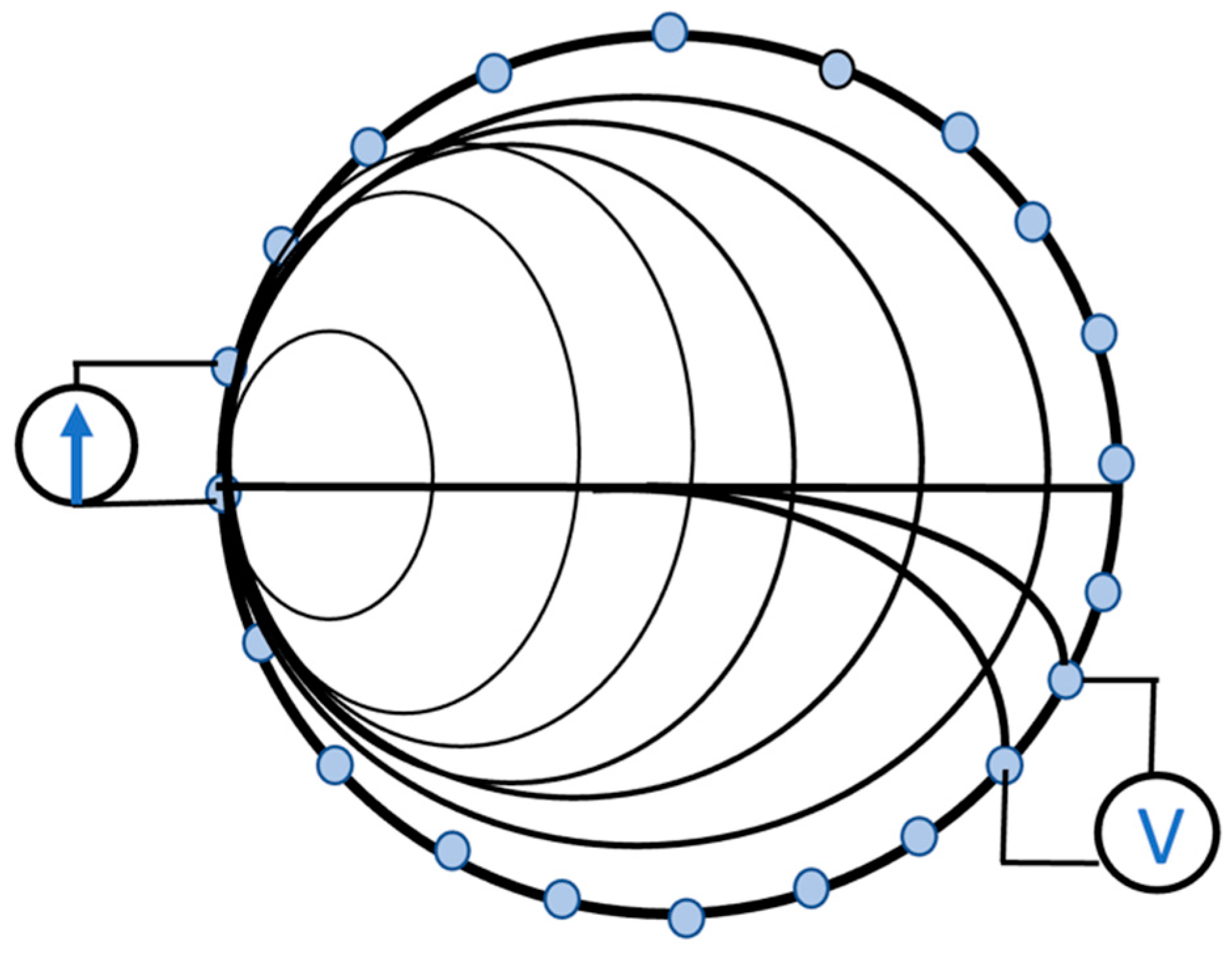
2.2.2. Electrical Resistance Tomography (ERT)

The primary aim of Electrical Resistance Tomography (ERT) is to image the fluids flowing through when the continuous phase is conductive, and the dispersed phase is less conductive or non-conductive. The electrodes are small and directly in contact with the fluid, or sometimes a conductive ring is also used [19]. In this technique, a pair of electrodes is usually excited. A combination of excitation currents is applied to determine the voltages between the electrodes. The obtained voltages are then used to construct the conductivity distribution, which, in turn, determines the distribution of the components present in the fluid. This method is highly sensitive near the wall of the vessel but poor in the centre of the measurement region [21]. Another method is to inject the current between the opposite electrodes. A typical ERT sensor is shown in Figure 7 [19].

Figure 7. An ERT sensor with a voltage measurement circuit around the periphery of a conductive ring. Reproduced with permission from ref. [19] and Copyright 2005 Elsevier Ltd.

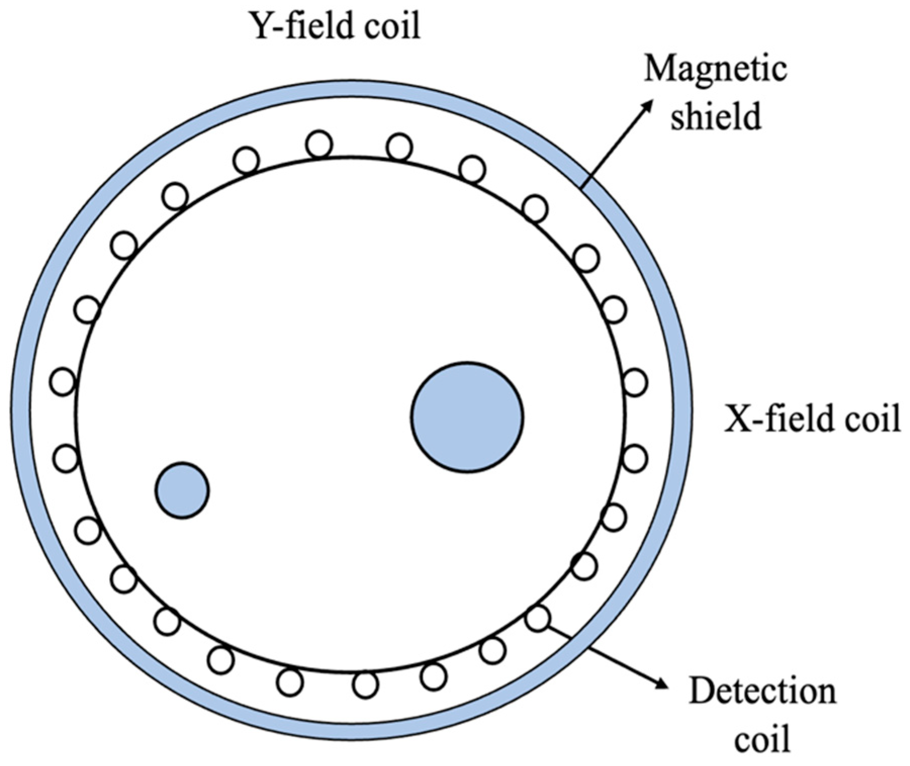
2.2.3. Electromagnetic Tomography (EMT)

The basic principle of electromagnetic tomography (EMT) is to determine the fraction of each component in a multi-phase flow using the permittivity of the fluid medium. This consists of a set of coils that produce a magnetic field in the measurement region within the pipe and a set of coils that detect the changes in the field due to changes in the permeability inside the pipe or vessel, as shown in Figure 8 [19]. Since water has a higher permittivity ($\mathsf{\epsilon }=80$) than oil, the sensor is more sensitive to water. A high excitation frequency is required to increase the signal strength from the sensor [24]. EMT is flexible in design, and there is no contact with the measurement region or sensing area. However, the image resolution of the EMT is poor and more work needs to be carried out in this field [19].

Figure 8. An EMT sensor with excitation and detection coils, along with a magnetic shield. Reproduced with permission from ref. [19] and Copyright 2005 Elsevier Ltd.

2.3. Gamma Densitometry

Gamma attenuation is a non-intrusive technique that is useful for measurements of components that have a sufficient difference in their density [25]. It works on the principle that the gamma beams from the radioactive source are attenuated depending on the absorption of radiation with matter. The degree of attenuation depends on the energy of the gamma beam and the density of the matter being absorbed [24,26].

The application of gamma-ray is limited to offshore and topside processes due to concerns over the use of a radioactive source. The main drawbacks of this method are flow regime dependence when measuring volume fractions of components and discontinuities in measurements [27].

The main components of the gamma-ray densitometer are a radioactive source providing a constant intensity, a detector, and a signal processing system [26]. The gamma source and the detector unit are located diametrically opposite each other with a collimator section to produce a narrow beam, as shown in Figure 9. The two main interactions employed are photoelectric and Compton scattering interactions.

Figure 9. Gamma densitometer with a gamma source and detector unit located diametrically opposite to each other with a collimator structure to ensure a narrow beam production. Reproduced with permission from ref. [28] and Copyright 2007 Elsevier Ltd.

In photoelectric phenomena, the photon ejected by the gamma-ray beam is completely absorbed, and its energy is used to ionize the absorbing atom and provide kinetic energy to the ejected electron. The photoelectric probability cross-section depends on the absorbing material’s atomic number (Z) and the incident photon’s energy €.

In Compton scattering, the photons collide with a loosely bound electron, thus giving off a part of the photon’s energy and becoming deflected through an angle $\mathsf{\theta }$. The Compton probability is directly proportional to the atomic number (Z) of the absorbing material [28]. The attenuation of mono-energetic gamma beams is given by the Beer–Lambert Law for a homogeneous material and is expressed as [26]

$$\mathrm{I}={\mathrm{I}}_0{\mathrm{e}}^{-\mathsf{\rho }\mathsf{\mu }\mathrm{x}}$$

(6)

where ${\mathrm{I}}_0$ is the incident intensity, $\mathrm{I}$ is the intensity after the beam has travelled a distance $\mathrm{x}$ in the absorbing material, $\mathsf{\mu }$ is the mass absorption coefficient, which is the ability of the material to absorb the radiations, and $\mathsf{\rho }$ is the density of the absorbing material [26].

For a two-phase oil–water flow, the geometric distribution of the two phases is in layers that are either parallel or perpendicular to the incident beam. The attenuation of the gamma radiation for the perpendicular distribution is given as [26]

$$\mathrm{I}={\mathrm{I}}_0{\mathrm{e}}^{\left[-\left({\mathsf{\rho }}_{\mathrm{o}}{\mathsf{\mu }}_{{}_{\mathrm{o}}}{\mathrm{x}}_{\mathrm{o}}+{\mathsf{\rho }}_{\mathrm{w}}{\mathsf{\mu }}_{{}_{\mathrm{w}}}{\mathrm{x}}_{\mathrm{w}}\right)\right]}$$

(7)

where ${\mathsf{\mu }}_{\mathrm{o}}$ and ${\mathsf{\mu }}_{\mathrm{w}}$ are the mass absorption coefficients of oil and water, respectively, and ${\mathrm{x}}_{\mathrm{o}}$ and ${\mathrm{x}}_{\mathrm{w}}$ are the path lengths of the beam in the oil and water phases, respectively [26]. Dual-energy gamma densitometry that measures the different components in a mixture depends not only on the densities but also on the distribution of the components if they are not mixed in the pipe and water salinity. To monitor and detect the salinity component of the water, we can couple the measurements obtained from the transmitted and scattered gamma radiation since they have different values to the interactions and the fluid medium [25].

2.4. Infrared Water-Cut Meter

The infrared water-cut meters rely on Near-Infrared (NIR) absorption spectroscopy. This water-cut meter can measure the water cut for the full range (0–100%) in transient conditions [29]. It is based on the large difference between the absorption of infrared radiation by crude oil and water [30]. There are certain peaks in the NIR spectrum, where water absorbs more energy at higher wavelengths than oil [31], as shown in Figure 10a [32]. A water-cut sensor based on IR spectroscopy exploits the differences in water and oil’s absorption properties [31].

Figure 10. (a) NIR spectrum depicting the differences in the absorption properties of oil and water. (b) Schematic diagram of the insertion probe of an infrared water-cut meter [32].

The insertion probe of the water-cut meter consists of a NIR emitter and detector on the opposite ends while the oil–water emulsion flows in between, as shown in Figure 10b [32]. The emitter transmits the NIR waves, and the detector converts the signals to a photocurrent value. There are sapphire windows that shield the radiation at both ends [7,32].

The water molecules contain O-H bonds and the hydrocarbon molecules do not, making it easy for the NIR waves to differentiate between them [33,34]. The NIR water-cut meter can distinguish between water, condensate, methanol, and gas at specific wavelengths [7,32].

Water cut can be calculated using the following equation [7]

$$\mathrm{W}\mathrm{C}=\left(\frac{{\mathrm{A}}_{\mathrm{o}\mathrm{w},\mathsf{\lambda }}-{\mathrm{A}}_{\mathrm{o},\mathsf{\lambda }}}{{\mathrm{A}}_{\mathrm{w},\mathsf{\lambda }}-{\mathrm{A}}_{\mathrm{o},\mathsf{\lambda }}}\right)100.$$

(8)

where ${\mathrm{A}}_{\mathrm{o}\mathrm{w},\mathsf{\lambda }}$ is the absorption of the oil–water mixture at wavelength $\mathsf{\lambda }$, ${\mathrm{A}}_{\mathrm{o},\mathsf{\lambda }}$ is the absorption of oil phase only, determined via calibration at wavelength $\mathsf{\lambda }$, and ${\mathrm{A}}_{\mathrm{w},\mathsf{\lambda }}$ is the absorption of water phase only, determined by calibration at wavelength $\mathsf{\lambda }$.

The main advantages of infrared water-cut meters include that they are unaffected by salinity and emulsions [7], relatively tolerant to changes in oil properties, and able to measure water-cut even in the presence of free gas [34]. One of the main drawbacks is that the contaminants present in the oil–water mixture can change the optical properties of the insertion probe in the water-cut meter, and thus require regular cleaning. Other disadvantages include that the absorption spectroscopy of the oil must be known, and if the flow velocity is too low, then upstream mixing is required to maintain the flow stream [7]. This technology can be used to measure gas–liquid flow.

2.5. Coriolis Flowmeter

Coriolis flow metering is a widely used technique for measuring industrial flow measurements [35]. Coriolis flowmeters provide the mass flow rate and density of the bulk fluid, which can be used to calculate the volumetric flow rate and water cut over the full range (0–100%). Calculation of the water-cut depends on factors such as the water density, operating surface pressure, and liquid density. The density of water should be greater than the density of the oil and the emulsion. Operating pressures below the bubble point generate entrained gas, which lowers the density of the emulsion and, in turn, reduces the water cut value. A Coriolis meter requires that the liquid density for a homogeneous oil–water emulsion lies between the oil and water density values [36].

A typical Coriolis meter consists of two flow tubes (i.e., the sensor element) oscillating 180° out of phase at their natural frequency [37], which is connected in series with process piping, and an electronic transmitter, which is responsible for controlling the flow tube vibration, as shown in Figure 11 [38]. The transmitter carries out the measurement calculations and finally relays the measured data to the user [38].

Figure 11. A Coriolis meter with two flow tubes through which fluid passes, and an electronic transmitter responsible for maintaining the vibrations in the tube and performing calculations [38]. Copyright 2019 Elsevier Ltd.

The flow tubes are typically 1–300 mm in diameter and oscillate at their natural resonant frequency according to a selected mode of mechanical vibration called the drive mode. The frequency of oscillation is 50 Hz–1 kHz, which depends on the geometry and stiffness of the flow tube, and is calculated by the overall mass of the system. The overall mass varies with the density of the fluid [39,40].

As the fluid passes through the flow tubes, it exerts a Coriolis force that opposes the tubes’ vibration. This Coriolis force creates a distortion or twist between the two legs of the sensor tubes. The magnitude of the twist is proportional to the mass flow rate. The phase is converted to time, which is proportional to the mass flow rate. The resonance frequency of the sensor tubes will also be affected by the fluid flowing through the tubes. Thus, the density of the fluid can be determined by the change in the resonance frequency [41]. Most of the Coriolis flowmeters also have a temperature sensor to compensate for the changes in the tube stiffness with temperature [42].

The advantages of Coriolis flowmeters are as follows: (1) they provide the correct reading for mass flow rate and density; (2) there is no need for multiple complex devices and flow computers to calculate and reach the final result; (3) the Coriolis flowmeter is bidirectional (i.e., it can handle the fluid flow in either direction without any adjustments); (4) they are extremely accurate (0.1% for steady flow rates); (5) it is easy to install since it has no moving parts. On the other hand, the limitations of the Coriolis flowmeters are as follows: (1) the capital cost is high and drastically increases with size [42]; (2) the introduction of gas and salinity in the process instantly affects the accuracy of water-cut measurements; (3) density-based measurements are limited to light oil due to the small difference between the densities of water and heavy oil [6]; (4) oil and water densities must be known; (5) the changes in oil and water densities with temperature must be known [7].

2.6. Ultrasonic Water-Cut Meters

Ultrasonic techniques are used to determine the composition of heterogenous mixtures for industrial applications [43]. This technique is still in the developing phase and has yet to be fully commercialized [7]. Ultrasonic meters can operate over the full water-cut range (0–100%). The main advantages of an ultrasonic water-cut meter are as follows: (1) it is easy to install; (2) less maintenance is required [44]; (3) it has the ability to analyze emulsions non-invasively; (4) it is non-hazardous to personnel (unlike gamma ray densitometry); (5) it has the ability to penetrate highly dense fluid mixtures [43]; (6) it has a low cost; (7) it is simple to operate; (8) temperature variations have less influence [45].

The main types of ultrasonic meters are the transit-time method, frequency-difference method, phase-difference method, cross-correlation method, and Doppler method [46].

Transit Time Method

The flowrate of a given mixture can be obtained by measuring the transit time of the of the ultrasonic wave in both directions. The difference between the transit times in both directions is linearly proportional to the flow velocity. If the flowrate is too low, the transit time difference (TTD) will be small as well. This difference can be as small as a few picoseconds, which can be difficult to measure within a given accuracy. This transit time ultrasonic flow meter is a new, improved method for water flowrate measurements. This meter consists of two transducers that are mounted coaxially, as shown in Figure 12. The upstream and downstream transducers are separated by a known distance, L. A piezoelectric crystal inside the upstream transducer sends an ultrasonic signal to the downstream one when subjected to an alternating voltage. This ultrasonic signal can travel in the direction of flow (downstream) and against the direction of flow (upstream), to be received by the opposite transducer in the time interval called transit time. The signal travels faster in the direction of flow and slowly against the flow. The difference between the two transit times is directly proportional to the flow velocity [44].

Figure 12. Schematic of transit yime flow meter—(1) inlet; (2) cable connector; (3) upstream transducer; (4) flow meter body; (5) downstream transducer; (6) outlet. Reproduced with permission from ref. [44] and Copyright 2016 MDPI.

To further explain the measurement parameters, assume the upstream and down stream transit time to be ${\mathrm{t}}_{\mathrm{u}\mathrm{p}}$ and ${\mathrm{t}}_{\mathrm{d}\mathrm{o}\mathrm{w}\mathrm{n}}$, which are given by Equations (9) and (10) respectively. c is the speed of sound, and transit time difference (TTD) is calculated by Equation (11) [44].

$${\mathrm{t}}_{\mathrm{u}\mathrm{p}}=\frac{\mathrm{L}}{\mathrm{c}-\mathsf{\nu }}$$

(9)

$${\mathrm{t}}_{\mathrm{d}\mathrm{o}\mathrm{w}\mathrm{n}}=\frac{\mathrm{L}}{\mathrm{c}+\mathsf{\nu }}$$

(10)

$$\mathrm{T}\mathrm{T}\mathrm{D}=\Delta \mathrm{t}={\mathrm{t}}_{\mathrm{u}\mathrm{p}}-{\mathrm{t}}_{\mathrm{d}\mathrm{o}\mathrm{w}\mathrm{n}}=\frac{2\mathsf{\nu }\mathrm{L}}{{\mathrm{c}}^2-{\mathsf{\nu }}^2}$$

(11)

Assuming ${\mathsf{\nu }}^2\ll {\mathrm{c}}^2$ (flow velocity, $\mathsf{\nu }$, is very small in comparison to speed of sound)

$$\Delta \mathrm{t}={\mathrm{t}}_{\mathrm{u}\mathrm{p}}-{\mathrm{t}}_{\mathrm{d}\mathrm{o}\mathrm{w}\mathrm{n}}=\frac{2\mathsf{\nu }\mathrm{L}}{{\mathrm{c}}^2}$$

(12)

which can be simplified as:

$$\mathsf{\nu }\approx \frac{{\mathrm{c}}^2\Delta \mathrm{t}}{2\mathrm{L}}$$

(13)

There are two models used for calculating the water volume fraction, ${\mathrm{V}}_{\mathrm{w}}$, given by Urick and Kuster–Toksöv. The common assumptions of the models are as follows: (1) the wavelength of the acoustic waves is much longer than the characteristic size of the dispersed particles/phase; (2) the multiple scattering effects of the sound field are negligible [47].

The Urick model uses a linear equation where $\mathsf{\varphi }=(1-{\mathrm{V}}_{\mathrm{w}})$

$$\mathsf{\rho }=\mathsf{\varphi }{\mathsf{\rho }}_{\mathrm{o}}+\left(1-\mathsf{\varphi }\right){\mathsf{\rho }}_{\mathrm{w}}$$

(14)

And the Kuster–Toksöv model uses [47]:

$$\frac{{\mathsf{\rho }}_{\mathrm{w}}-\mathsf{\rho }}{{\mathsf{\rho }}_{\mathrm{w}}+2\mathsf{\rho }}=\mathsf{\varphi }\frac{{\mathsf{\rho }}_{\mathrm{w}}-{\mathsf{\rho }}_{\mathrm{o}}}{{\mathsf{\rho }}_{\mathrm{o}}+2{\mathsf{\rho }}_{\mathrm{o}}}$$

(15)

The models can be simplified and expressed as a general quadratic equation [47]:

$$\mathrm{A}{\mathsf{\varphi }}^2+\mathrm{B}\mathsf{\varphi }+\mathrm{C}=0$$

(16)

where

$$\mathsf{\varphi }=\frac{-\mathrm{B}\pm \sqrt{{\mathrm{B}}^2-4\mathrm{A}\mathrm{C}}}{2\mathrm{A}}$$

(17)

The solution of the above quadratic equation yields two roots, and only the root corresponding to $0\le \mathsf{\varphi }\le 1$ is used.

The coefficients $\mathrm{A}$, $\mathrm{B}$ and $\mathrm{C}$ are listed in Table 1 below [47,48].

Table 1. Coefficients of quadratic equation.

Coefficient	Urick Model	Kutser–Toksöv Model
$\mathrm{A}$	$(\mathrm{o}-\mathrm{r}\mathrm{w})(1-\mathrm{r})$	$(\mathrm{o}-\mathrm{r}\mathrm{w})(1-\mathrm{r})$
$\mathrm{B}$	$2\mathrm{r}\mathrm{w}-\mathrm{o}-{\mathrm{r}}^2\mathrm{w}$	$2\mathrm{r}\mathrm{w}-\mathrm{o}+{\mathrm{r}}^2\mathrm{w}+2\mathrm{r}(1-\mathrm{o}-\mathrm{r})$
$\mathrm{C}$	$\mathrm{r}(1-\mathrm{w})$	$\mathrm{r}(1+2\mathrm{r})(1-\mathrm{w})$

where $\mathrm{r}={\mathsf{\rho }}_{\mathrm{o}}/{\mathsf{\rho }}_{\mathrm{w}}, \mathrm{o}={\mathrm{c}}^2/{\mathrm{c}}_{\mathrm{o}}^2, \mathrm{w}={\mathrm{c}}^2/{\mathrm{c}}_{\mathrm{w}}^2$.

Thus, the water cut is:

$$\mathrm{W}\mathrm{C}=100\times \left(1-\mathsf{\varphi }\right)$$

$$\mathrm{W}\mathrm{C}=100\%\times \left(1-\frac{-\mathrm{B}\pm \sqrt{{\mathrm{B}}^2-4\mathrm{A}\mathrm{C}}}{2\mathrm{A}}\right)$$

(18)

Some of the disadvantages of the ultrasonic meter are: (1) a high capital cost, (2) transit time meters are sensitive to particulates and impurities, (3) they provide errors even with small gas bubbles, (4) Doppler meters are also sensitive to changes in concentration, temperature and density, (5) these meters do not work well with slurries and other highly concentrated mixtures [49], (6) water and oil densities should be known, and their changes with temperature must also be known, (7) the water and oil speed of sound should be known and, finally, (8) in-line testing is required for a smooth performance [7].

2.7. Microwave Sensor

Microwave-based measurements are non-intrusive, non-destructive and can measure from a short distance using low-power penetration waves without any health hazards to personnel. Thus, they offer minimal disruption to the flow in the pipe. They work based on the variations in the permittivity in the fluid composition [50,51]. Microwave sensors can detect a wide range of samples varying in viscosity, density and permittivity, and the accuracy of the measurements is not affected by these factors [52]. The microwave method has the ability to perform non-contact, high-resolution measurements in real-time. They have a low external influence in comparison to other techniques and are easy to install [52]. Microwave-based methods can be broadly categorized as wave resonance, reflection, and transmission line methods [4].

2.7.1. Microwave Resonator

A resonator consists of a section of a transmission line that is shorted (i.e., open on both ends). There are different resonators depending on the type of transmission line being used, such as coaxial, microstrip, stripline, slot line, or cavity resonators. The material under test (MUT) or object is brought into contact with a part of the electromagnetic field when used as a sensor. As a result, the resonance frequency and the quality factor will change with changes in the permittivity of the object [51,53]. The microwave resonance technology contains energy peak resonances at the fixed frequencies at which the sensor is designed to operate when acquiring the volume fraction of the flow [52,54]. This method has a low salinity tolerance, and no resonance will occur if the water content is too high [52].

Resonant Cavity Sensor

A microwave resonant cavity is a metallic cavity that can be cylindrical or any other shape (rectangular waveguide cavities or microstrip). It is constructed with both ends open, as shown in Figure 13. Here, ‘a’ and ‘d’ denote the radius and height of the cylindrical cavity [4]. It is filled with a fluid under test [55]. The cavity confines the electromagnetic waves in the microwave band and resonates at these frequencies [50]. The cavity is bulky [56], and the resonance frequency shows a change with a slight difference in the water content of the fluid [55]. Waveguide cavity sensors are popular due to their high quality-factor and sensitivity and are in direct contact with the material under test [56]. Thus, a resonant cavity could be used to detect the changes related to the total complex permittivity of the fluid, consisting of oil and water phases, indicated by a shift in the resonance frequency pattern inside the cavity [50].

Figure 13. Cylindrical cavity resonator. Reproduced with permission from ref. [4] and copyright 2018 Elsevier Ltd.

2.7.2. Transmission Sensors

The basic setup of a transmission sensor consists of two horn antennas, a transmitter and a receiver. The material under test (MUT) is placed between the two antennas so that a microwave signal of a fixed frequency is sent through a fluid mixture containing oil and water components, which produces different attenuation peaks. These peaks relate to the water content present in the emulsion. The attenuation or the phase shift is thus measured [50,53]. Such sensors are used for the measurement of liquids or films. They are similar to resonator sensors but a better fit for high-loss materials [53]. The sensitivity of these sensors is lower than the resonator sensors, and they are prone to contamination of the surface from which the fringing field arises [57].

2.7.3. Reflection Sensors

A reflection sensor works by measuring the reflection coefficient of a wave reflected from the transmission end of the line. It is designed so that the fringing field is in contact with the object, and thus leads to a change in the reflection coefficient. An example of this type of sensor is the open-ended coaxial sensor [53,57].

2.8. Conductance Method

The conductance method is based on the large difference in the conductivity of water and crude oil [9]. There are many types of conductance sensors, such as arc-type conductance sensors with guard electrodes, ring-shaped conductance array probes, and multiple electrode sensors. These sensors have the advantages of a fast response, simple structure, ease of implementation and good reliability [58]. Water cut can be calculated using Maxwell’s formula [59]. If the conductivity of the oil–water emulsion is ${\mathsf{\sigma }}_{\mathrm{m}}$ and the conductivity of water is ${\mathsf{\sigma }}_{\mathrm{w}}$, then the ratio of ${\mathsf{\sigma }}_{\mathrm{m}}$ to ${\mathsf{\sigma }}_{\mathrm{w}}$ can be obtained using Maxwell’s equations [60].

$$\frac{{\mathsf{\sigma }}_{\mathrm{m}}}{{\mathsf{\sigma }}_{\mathrm{w}}}=\frac{2\mathsf{\beta }}{\left(3-\mathsf{\beta }\right)}$$

(19)

where $\mathsf{\beta }$ is the volume fraction of the continuous conductive phase in a two-phase flow.

A conductance probe is a type of electrical sensor used to determine the water cut in multi-phase flows. Chen et al. [61] developed a conductance-probe-based well-logging instrument, as shown in Figure 14. Its response is combined with the total flow rate to determine the water cut in a two-phase flow in a vertical well. A probe arm is installed on the shaft of the instrument. It can be opened or withdrawn with the help of a motor driver. The conductance probe is installed on this probe arm, and its tip is directed towards the incoming flow. The conductance probe consists of a stainless needle, an insulation layer, and a stainless shell. The shell is separated from the needle with the help of the insulation layer. When the probe arm is in the open position, the conductance probe records the varying conductivities of the emulsion using a conductance telemetry circuit. The response of this probe is recorded and transmitted using a logging cable. A turbine instrument is connected to the conductance probe to determine the total flow rate. The response from both these instruments is used to calculate the water cut [61].

Figure 14. Conductance-probe-based well-logging instrument [61]. Copyright 2015 IOP Publishing Ltd.

3. Laboratory Offline Methods

3.1. Karl Fisher Titration

The Karl Fisher is a highly precise analytical method used to determine the amount of water in oil. It relies on the oxidation of sulphur dioxide with iodine in the presence of water. It is based on the Bunsen reaction:

$${\mathrm{I}}_2+2{\mathrm{H}}_2\mathrm{O}+\mathrm{S}{\mathrm{O}}_2\to 2\mathrm{H}\mathrm{I}+{\mathrm{H}}_2\mathrm{S}{\mathrm{O}}_4$$

After adding an iodine-containing reagent, the endpoint of the titration is calculated amperometrically by detecting the amount of iodine present in the mixture [62]. The water content is calculated using the standard Karl Fischer reaction:

$${\mathrm{H}}_2\mathrm{O}+{\mathrm{I}}_2+[\mathrm{R}\mathrm{N}\mathrm{H}]\mathrm{S}{\mathrm{O}}_3\mathrm{C}{\mathrm{H}}_3+2\mathrm{R}\mathrm{N}\to [\mathrm{R}\mathrm{N}\mathrm{H}]\mathrm{S}{\mathrm{O}}_4\mathrm{C}{\mathrm{H}}_3+2[\mathrm{R}\mathrm{N}\mathrm{H}]\mathrm{I}$$

where $\mathrm{R}\mathrm{N}$ represents a base, and iodine and water react in a 1:1 mole ratio using anhydrous methanol as a solvent [63]. There are two different techniques for water determination by the Karl Fischer method, including volumetric KF titration and Coulometric KF titration.

3.1.1. Volumetric Karl Fischer Titration

In the volumetric titration method, iodine is added using a burette to the solvent in the titration flask containing the sample [64]. The amount of water that is present is quantified from the volume of iodine consumed [65]. This method is preferred when the sample size is large and moisture content is 2% and above [66].

3.1.2. Coulometric Karl Fischer Titration

In this method, the sample is added to an electrolytic solution containing $\mathrm{S}{\mathrm{O}}_2$, a base, and a solvent in a titration cell. The iodine-containing reagent is released by electrolytic oxidation by the induction of an electric current. The amount of water present is quantified by the total charge passed [64]. This method is suited to samples containing 1% or less water [66]. The Karl Fischer titration has the advantages of high accuracy as it is based on a chemical reaction that depends on the presence of water, is specific for water determination as it can be used for volatile and non-volatile substances, a small amount of sample is needed to perform the titration, and it has a wide measurement range, from 0.001 to 100%, where smaller percentages of up to 1% are suited to coulometric titration and samples with more than 2% water are tested with volumetric titration. It is suitable for determining water in solids, liquids and gases, and is simple and requires less sample preparation and a shorter analysis time. On the other hand, the Karl Fischer titration has the disadvantage of high solvent consumption (in the case of volumetric). Strong acids, ketones, aldehydes, and metal peroxides are not suitable for this technique as their reaction with the solvent methanol produces water, and this titration method depends on a redox reaction. Hence, any compound within the sample that is an active redox chemical reagent can react with iodine and provide incorrect values. Coulometric titration is only suitable for samples containing a small amount of water, as a larger amount of this sample may provide wrong results in addition taking a much longer time to generate the results [67,68].

3.2. Dean-Stark Distillation

The first continuous refluxing method was developed by Dean and Stark, which has now become the reference method for determining the water content of a sample. This method is commonly employed for water determination in herbs, spices and petroleum products [69]. The water present in the sample is vaporized using a solvent (e.g., toluene, xylene). The solvent is chosen such that it is immiscible with water at room temperature but forms an azeotropic mixture at the boiling point [69]. Water and solvent condensates are collected in a graduated glass cylinder. Due to the density contrast, the two liquids separate, making it possible to determine the volume of water being extracted. Once the solvent has condensed, it is returned to the heating flask, where it is re-circulated until no more water can be extracted [70]. Figure 15 shows the Dean–Stark extraction apparatus for the gravimetric determination of water [70].

Figure 15. Dean–Stark extraction apparatus for the gravimetric determination of water [70]. Copyright 2019 Elsevier Ltd.

The procedure is generally very accurate and simple to carry out and does not require much attention during distillation [71]. The main limitation of this method is that it is a time- and energy-consuming method since it has to be carried out until the receiver’s water level does not increase more than 0.1 mL in 30 min, or until the distillation has been carried out for 2 h [69]. Water from the sample evaporates when it is not immediately set up in the extractor at room temperature. There is a loss of water due to joints not being tight in the extraction flask or from insufficient flow to the condenser, and inaccurate results for water determination arise when the solvent has not been thoroughly dried or when the extraction time is not long enough [71]. The same distillation concept is also used in rotary evaporator (rotovap) apparatus where the vaporized water from an oil sample is condensed, collected, and used to calculate the water content.

3.3. Centrifugal Separation

The centrifuge method used to determine water in crude oil is also known as the Basic Sediment and Water (BS &W) process. It is one of the oldest and most widely used techniques. This test involves spinning equal volumes of oil and solvent placed in a centrifuge tube, which is heated to $60 °\mathrm{C}\pm 3 °\mathrm{C}$ for a specified amount of time until all the water and heavier sediments settle at the bottom of the tube. After centrifugation, the volume of the water–sediment layer at the bottom is measured [72,73].

The equipment used and skilled labour required for this procedure is less expensive than Karl Fischer titration [74]. However, this method usually understates the water content for most types of oils. Hence, this method does not have good accuracy [72].

4. Summary of Water-Cut Measurement Techniques

The properties of an oil–water emulsion that are used to detect the water cut are summarized below. Each technique has its own advantages and limitations, and we have to be mindful of all the parameters of each technique before selecting a particular one. A qualitative comparison/summary of the discussed techniques is presented below in Table 2.

Table 2. Comparison of different water-cut sensing techniques.

Measurement Techniques	Range	Advantages	Limitations	Application
Capacitance-based water-cut meters [6,7]	50–80%	Simple design and structure. Insensitive to water conductivity. Fast response speed. High sensitivity. Low cost.	Works best when the water cut is low. Works for water-in-oil emulsion where oil is the continuous phase. Impact of density, temperature and salinity. Frequent in-line calibration required.	Oil–water two-phase flow (petroleum industry)
Electrical Capacitance Tomography (ECT) [19,20,21,23]	<40%	Rapid response. Robust. No radiation, Relatively low cost. High-temperature and pressure tolerance. Non-invasive and non-intrusive.	Challenges in image reconstruction. Electrodes must have a large surface area to provide sufficient signal. Challenge in detecting changes in the order of 10−15F in the presence of standing capacitance and stray capacitance of the order of 100 pF. Only suitable for oil-continuous flows.	Gas/oil flows in oil pipelines, gas/solid flows in pneumatic conveyors and gas/solid distribution in fluidized beds.
Electromagnetic Tomography (EMT) [19,24]	N/A	Flexibility in sensor design. No contact with the sensing zone.	Requires a high excitation frequency to receive a signal from sensor. Image resolution is poor.	Multiphase flow in the offshore industry.
Electrical Resistance Tomography (ERT) [9,21,24]	>40%	Electrodes are relatively small.	Only suitable for continuous water flows. Only suitable for measurement in vertical pipes. Impacted by temperature and mineralization degree.	Oil–water two-phase flow in vertical pipes.
Gamma Densitometry [26,27]	0–100%	Non-intrusive technique. High penetration abilities. Less expensive in comparison to neutron densitometry. Produces mono-energetic rays without intensity fluctuations as opposed to the X-ray attenuation technique.	Flow regime dependence. Discontinuity in measurement. Uses a radioactive source.	Gas hold-up, oil–water flow in horizontal and slightly inclined pipes.
Infrared water-cut meter [7,34]	0–100%	Unaffected by salinity and changes in oil and water densities. Relatively tolerant to changes in oil property. Measures water-cut even in the presence of free gas.	Requires regular cleaning of the insertion probe. Absorption spectroscopy of the oil must be known. Upstream mixing is required if flow velocity is low.	Multi-phase flow in horizontal wells.
Coriolis flowmeter [6,7,42]	0–100%	Multi-variable output: flowrate, temperature and density. Bi-directional, and can handle flow in either direction. No moving parts and less maintenance, thus enhancing personnel safety.	Capital cost is high. Free gas and salinity affect water cut values. Oil and water densities must be known. Changes in oil and water densities with temperature must be known.	Monitoring density of catalyst in copolymer production. Monitoring TiO2 concentration in paper manufacturing; monitoring flowrates of chemicals (e.g., ethylene); petroleum industry.
Ultrasonic water-cut meter [7,43,44,49]	0–100%	Easy to install; inexpensive. Less maintenance. Penetrates highly dense mixtures. Non-hazardous to personnel. Non-invasive technique. It has bi-directional flow capabilities.	High capital cost. Transit-time flowmeters are sensitive to the presence of particulates and impurities. Water and oil densities must be known and change with temperature. Not suited for slurries and dense mixtures. Doppler method is sensitive to changes in temperature, concentration and density.	Oil–water emulsions.
Microwave sensor [9,50,51,52,56]	0–100%	High accuracy. Non-intrusive, non-destructive. Safe for personnel. Easy installation and fabrication. Low cost; small size. Contactless; real-time measurement. No phase-inversion phenomena.	Affected by salinity. A high degree of specialization. Several parameters (moisture, temperature, density) affect the measurement.	Multi-phase fluid flow in the oil industry.
Conductance sensor [58,61]	0–100%	Fast response. Ease of implementation. Good reliability. Simple structure.	Variations in water conductivity affect measurement values. Inaccurate values due to complex flow regimes and slippage between oil and water.	Oil–water two-phase flow; gas–liquid two-phase flow.
Karl Fischer titration [67,68]	0.001–100%	High accuracy and specificity. Simple method. Less time-consuming. Suitable for water content determination in solids, liquids and gases.	High solvent consumption. Unsuitable for compounds containing active redox chemical reagents. Coulometric titration is suitable only for samples containing small amounts of water.	Quality control in the pharmaceutical, food and chemical industries.
Dean–Stark distillation/Rotary Evaporator [69,71]	N/A	High accuracy. Simple method.	Time and energy consuming process. Inaccurate results if the solvent is not dried properly. Incorrect reading can occur when there is a loss of water due to joints in the extraction flask not being vapor-tight or due to an inadequate amount of water flowing to the condenser.	Water determination in herbs, spices, food, petroleum products and crude oil.
Centrifugal separation [72,74]	0–100%	Equipment used and personnel needed is less expensive than KF titration.	Provides a lower value of water content; low accuracy.	Secondary or tertiary production of crude oil.

5. Trends and Future Research Developments

After a review of the most common methods available for WC measurement, the present and future of WC measurements in the industry are briefly discussed. Oil is still a major source of energy in many countries, and developing new optimizations factors for production could make the industry more efficient and sustainable. With a slight increase in operational measurement efficiency, oil and gas companies can produce the same amount of energy at a lower cost and with less energy consumption, resulting in a lower environmental impact. Furthermore, the oil and gas industry’s rapid digitalization has paved the way for the emergence of the ‘digital oilfield’, a process that is gaining traction. The digital oilfield allows for all operational data to be monitored, evaluated, and used in real-time, owing to the upsurge in data analytics, cloud computing and big data, resulting in safer and more sustainable decisions. Some of the current and most prominent hotspots of research for water-cut measurements are discussed below.

5.1. Computer Vision

Computer vision is a fast-growing research area with many applications, including measuring water cut. A novel, non-contact prototype has been developed and tested by Q. Liu et al. [3]. In this method, the oil–water phases were separated out by electric dehydration. A mixture with a clear color difference was obtained. A low-cost image sensor was used to photograph RGB images of this mixture into a grayscale image. The grayscale-accumulated value difference (IGAVD) algorithm was used to detect the pixels of each component in the oil–water mixture and obtain their coordinate positions. The water content was then determined by image plane correspondence.

The main factor affecting the accuracy and success of this method is light brightness. The image acquisition range function needs to be adjusted to cancel out the noise from other environmental factors. Features such as contrast, brightness and robustness need to be considered when considering a light source. Another limitation of this method is that transparent containers should be used after separating the oil–water emulsion [3].

5.2. Artificial Intelligence in Oil and Gas

Artificial Intelligence (AI) has been in use since the 1950s, and is rapidly progressing through various algorithms, such as Artificial Neural Network (ANN), Fuzzy logic, Support Vector Machine (SVM), Genetic Algorithm, and Hybrid Intelligent System (HIS). AI concepts have been widely used in the oil and gas industry, from intelligent drilling, production, and pipeline to the refinery, and will continue to be the leading research area in future. AI is being used in oil and gas to predict oilfield production and the optimization of the development plan, as well as being utilized for water content measurements [75].

The prediction method for oil production/forecasting is increasingly attracting attention. When combined with AI methods such as neural networks with fuzzy logic, the predictions result in a better fitting accuracy with the production data. These data are used to estimate the current status of an oilfield, such as its cumulative production volume and injection volume, and predict the future trends in the water cut rise rate, oil recovery rate, etc. Algorithms such as the Graph Neural Network (GNN) and Improved Particle Swarm Optimization (IPSO) have been employed to determine the water cut and oil production. However, there is the potential to apply more practical algorithms to the real-time water-cut measurement data. This has yet to be explored for the efficient development and dynamic prediction of an oilfield. Accurate water-cut measurements play a significant role in the success of the development of oil production/forecasting predictions using AI approaches [75].

Oil field development plan optimization is crucial as it directly affects the lifespan of an oilfield. Long-term water injections have caused the oilfields to enter a phase characterized by high water cut. Various algorithms have been adopted to evaluate and optimize the development of plans aiming to improve the production rate by taking the economic factors into consideration. The current methods of analysis should be further improved by more accurate and reliable water-cut measurement data. AI is the current and future research hotspot. Every AI algorithm has its own limitations but selectively choosing an algorithm for a specific application is the key to solving problems. Collaboration at all levels and regions and the capacity to utilize the big data of oil fields is needed for the transition from digital oilfields to AI oilfields [75].

5.3. Soft Computing

Soft computing is a set of algorithms that aim to predict the tolerance level for imprecision and uncertainty. It covers a range of computational techniques in artificial intelligence, computer science and machine learning. Soft computing techniques are also being used for multi-phase flow measurement, particularly to determine phase flowrates, phase fraction, and the identification of flow regimes. These computational techniques, when combined with traditional sensors such as ultrasonic sensors, electrical sensors, optical sensors, differential pressure devices and Coriolis flowmeters, provide an optimized and effective solution. The main feature of soft computing techniques is their ability to provide effective methods to model complex multi-phase flows, which are difficult to interpret, and hence estimate the phase fractions. In this way, sensor fusion extends the accuracy, measurement range and suitability of the above-mentioned traditional sensors. It should be noted that the evaluation of models is a critical step in achieving better results. Therefore, careful consideration of the input variable selection method and model evaluation are vital in the successful development of data-driven models for multi-phase flows. These techniques may provide an intelligent and cost-effective solution. However, it is worth mentioning that the calibration of such multi-phase meters (estimating phase fractions) is a challenging issue that needs to be tackled [5].

5.4. Metamaterial THz EIT-like Sensor

Metamaterials are a new class of functional materials that are fabricated with unique properties, such as super lensing and negative refraction. A THz Electromagnetically Induced Transparency (EIT) metamaterial sensor was developed by Song et al. [76] to detect water in oil–water emulsions. These materials are sensitive to changes in the permittivity of the surrounding medium. It was found that the sensitivity increased with the increasing distance between the bright and dark modes, similar to a weakened plasma resonance. The sensor exhibited a red-shifted resonance frequency response when the water content in the emulsions varied from 60 to 98%. The absolute errors were less than 1%. This method was proven to overcome the limitation associated with the Terahertz Spectroscopy of being strongly attenuated by a water layer and low-quality factor (Q-factor). However, for this method to develop an EIT-like effect, a significant difference in the Q-factors or the full-width-at-half-maximum of the bright and dark resonance modes is required [76].

5.5. All Optical Detection

A new method to measure the full range of water cut was proposed by Lu et al. [77] using an all-optical detection method. This comprises a non-contacting laser source and a laser interferometer, which works as the receiver and achieves, hence the name, all-optical detection. The method works by irradiating an optically absorbing surface with a short pulse, high-energy laser, which excites the ultrasonic P-waves via thermoelastic expansion. The resulting waves are detected by a second laser coupled with an optical interferometer. The data from this interferometer are then recorded by an oscilloscope. The data are then further processed to determine the time the ultrasonic P-waves take to pass through a sample by detecting when the first significant peak appears. The water content is thus measured by the different ultrasonic P-waves velocities corresponding to different water contents. It was found that the P-wave velocity increases with the increase in water content. While this method has great potential in the industry, it still needs to be studied further to improve the precision of real-time detection and the portability of the detection device [77].

5.6. Nuclear Magnetic Resonance (NMR)

NMR is a robust online flow measurement technique that is fast and reliable, and has high sensitivity [78]. It has the ability to probe systems non-invasively and requires few samples for measurement. It is unaffected by salinity, temperature and emulsion characteristics [79]. This technique measures the response of the nuclei of atoms when placed in a magnetic field. Some nuclei responses depend on whether they possess a property known as “spin”. These spinning nuclei can interact with the external magnetic field and produce measurable signals. The most commonly used nuclei are hydrogen atoms, as they have the largest magnetic moment and are abundant in water and hydrocarbons. An NMR tool polarizes the hydrogen atoms present in the crude oil and water in the presence of a magnetic field and measures the time it takes for these protons to return to equilibrium. This time is recorded as the transverse relaxation time. This relaxation time is shorter for bitumen compared to water, as the movement of the protons in crude oil is limited due to high viscosity [80,81]. The NMR measurement cycle, known as the Carr–Purcell–Mei-boom–Gill pulse sequence (CPMG), generates a spectrum of amplitude versus relaxation time, and the water content can be calculated by measuring the peak area of water in the spectrum [80,82]. While this technique has promising applications for the online detection of water content, it is also accompanied by the risk of magnetic disturbances requiring magnetic shielding. It is costly and requires a statistical approach to correlate the data obtained from the spectrum with the characterization of crude oil [83].

5.7. Intensifying Device (ID) in Mobile Well Production Treatment Units

Flow measurement in the presence of emulsions is challenging [84]. A design has been reported to enhance emulsion separation, leading to more accurate separation and water-cut measurements [85]. The new technique is based on the usage of an Intensifying Device (ID) in mobile well production treatment (MWPT) [85]. The study involved testing an intensifying device on a mobile well production treatment unit for emulsion separation [85]. In this design, cassettes were positioned within the unit’s sump, with two distinct distances between the plates: 5 mm (standard design) and 2.5 mm. The experiments involved several variations in process conditions, such as the direction of fluid entry to the sump, temperature, and flow rates. It was found that a smaller distance between the plates (2.5 mm) in the intensifying device led to turbulent diffusion, which improved the emulsion separation process. This resulted in a more effective treatment of oil. The research demonstrated that the desalting process was more efficient at higher temperatures (70 °C) than lower temperatures (60 °C). This suggests that higher temperatures promoted more efficient oil and water separation. The study produced novel results showcasing that the use of intensifying devices with a smaller distance (2.5 mm) between the plates resulted in improved oil treatment, leading to more accurate water-cut measurements in the presence of emulsions [85].

6. Conclusions

Water cut is an important parameter in the oil and gas industry, which directly affects the many aspects of crude oil production and is now gaining more and more attention. It is very important for quality control in the production of an oilfield and reduces the energy and time consumption. New water-cut measurement technologies should be evaluated based on their accuracy, working range, sensor configuration, maintenance requirements and cost.

This review discusses and includes the principles of some of the most commonly employed methods for water-cut measurements and provides some background on recent and future technologies. Different techniques are presented and compared based on their optimum working range, along with their advantages and limitations.

The future development trends in water-cut measurement techniques are also predicted and discussed. New research techniques such as soft computing algorithms, functional materials like metamaterials, computer vision, and optical detection methods are progressively being developed, which have proven to increase the reliability and sensitivity response in water-cut sensing.

Each measurement technique outlined in this review has its own characteristics, and users should be equipped with sufficient knowledge about their process specifications and chosen technology. This review will provide a roadmap for users that will help them in making a better decision as to which sensor best fits their requirements.

References

- Yang, Y.; Xu, Y.; Yuan, C.; Wang, J.; Wu, H.; Zhang, T. Water cut measurement of oil–water two-phase flow in the resonant cavity sensor based on analytical field solution method. Measurement 2021, 174, 109078. [Google Scholar] [CrossRef]
- Guowang, G.; Dasen, H.; Hua, L.; Wang, F.; Li, Y. Research Status and Development Trend of Water Cut Detection Methods for Crude Oil. J. Phys. Conf. Ser. 2021, 1894, 012093. [Google Scholar] [CrossRef]
- Liu, Q.; Chu, B.; Peng, J.; Tang, S. A visual measurement of water content of crude oil based on image grayscale accumulated value difference. Sensors 2019, 19, 2963. [Google Scholar] [CrossRef] [PubMed]
- Sharma, P.; Lao, L.; Falcone, G. A microwave cavity resonator sensor for water-in-oil measurements. Sens. Actuators B Chem. 2018, 262, 200–210. [Google Scholar] [CrossRef]
- Yan, Y.; Wang, L.; Wang, T.; Wang, X.; Hu, Y.; Duan, Q. Application of soft computing techniques to multiphase flow measurement: A review. Flow. Meas. Instrum. 2018, 60, 30–43. [Google Scholar] [CrossRef]
- Ametek Drexelbrook. What Criteria to Consider in Selecting a Water Cut Monitor Known as Basic Sediment and Water Meter (BS&W). Available online: https://escventura.com/manuals/ref_bswWaterCut_an.pdf (accessed on 2 October 2022).
- Castrup, S. Comprehensive Analysis of Water Cut Metering Accuracies. In Proceedings of the SPE Western Regional Meeting, Virtual, 20–22 April 2021. [Google Scholar]
- Yurish, S.Y. Advances in Measurements and Instrumentation: Reviews Book Series; IFSA Publishing, S.L.: Barcelona, Spain, 2018; Volume 1, pp. 152–153. [Google Scholar]
- Kong, W.; Li, H.; Xing, G.; Kong, L.; Li, L.; Wang, M. A Novel Combined Conductance Sensor for Water Cut Measurement of Low-Velocity Oil-Water Flow in Horizontal and Slightly Inclined Pipes. IEEE Access 2019, 7, 182734–182757. [Google Scholar] [CrossRef]
- ZelenTech. How to Select a Watercut Monitor. 2011. Available online: https://www.zelentech.co/blog/posts/how-to-select-a-watercut-monitor/ (accessed on 6 August 2022).
- Liu, X.; Qiang, X.; Qiao, H.; Ma, G.; Xiong, J.; Qiao, Z. A theoretical model for a capacitance tool and its application to production logging. Flow. Meas. Instrum. 1998, 9, 249–257. [Google Scholar] [CrossRef]
- Golnabi, H.; Azimi, P. Design and Performance of a Cylindrical Capacitive Sensor to Monitor the Electrical Properties. J. Appl. Sci. 2008, 8, 1699–1705. [Google Scholar] [CrossRef]
- Li, L.; Kong, L.; Xie, B.; Fang, X.; Kong, W.; Liu, X.; Wang, Y.; Zhao, F. The Influence on Response of a Combined Capacitance Sensor in Horizontal Oil–Water Two-Phase Flow. Appl. Sci. 2019, 9, 346. [Google Scholar] [CrossRef]
- Da Silva, M.J.; Hampel, U. Capacitance wire-mesh sensor applied for the visualization of three-phase gas-liquid-liquid flows. Flow. Meas. Instrum. 2013, 34, 113–117. [Google Scholar] [CrossRef]
- Da Silva, M.J.; Schleicher, E.; Hampel, U. Capacitance wire-mesh sensor for fast measurement of phase fraction distributions. Meas. Sci. Technol. 2007, 18, 2245–2251. [Google Scholar] [CrossRef]
- Assima, G.P.; Larachi, F.; Schleicher, E.; Schubert, M. Capacitance wire mesh imaging of bubbly flows for offshore treatment applications. Flow. Meas. Instrum. 2015, 45, 298–307. [Google Scholar] [CrossRef]
- Liu, X.; Hu, J.; Xu, W.; Xu, L.; Xie, Z.; Li, Y. A new cylindrical capacitance sensor for measurement of water cut in a low-production horizontal well. J. Phys. Conf. Ser. 2009, 147, 012002. [Google Scholar] [CrossRef]
- Reinecke, N.; Petritsch, G.; Schmitz, D.; Mewes, D. Tomographic Measurement Techniques - Visualization of Multiphase Flows. Chem. Eng. Technol. 1998, 21, 7–18. [Google Scholar] [CrossRef]
- Ismail, I.; Gamio, J.C.; Bukhari, S.F.A.; Yang, W.Q. Tomography for multi-phase flow measurement in the oil industry. Flow. Meas. Instrum. 2005, 16, 145–155. [Google Scholar] [CrossRef]
- Thorn, R.; Johansen, G.A.; Hjertaker, B.T. Three-phase flow measurement in the petroleum industry. Meas. Sci. Technol. 2013, 24, 012003. [Google Scholar] [CrossRef]
- York, T. Status of electrical tomography in industrial applications. J. Electron. Imaging 2001, 10, 608. [Google Scholar] [CrossRef]
- Wang, H.X.; Zhang, L.F. Identification of two-phase flow regimes based on support vector machine and electrical capacitance tomography. Meas. Sci. Technol. 2009, 20, 114007. [Google Scholar] [CrossRef]
- Li, Y.; Yang, W.; Xie, C.-G.; Huang, S.; Wu, Z.; Tsamakis, D.; Lenn, C. Gas/oil/water flow measurement by electrical capacitance tomography. Meas. Sci. Technol. 2013, 24, 074001. [Google Scholar] [CrossRef]
- Hansen, L.S.; Pedersen, S.; Durdevic, P. Multi-Phase Flow Metering in Offshore Oil and Gas Transportation Pipelines: Trends and Perspectives. Sensors 2019, 19, 2184. [Google Scholar] [CrossRef]
- Sætre, C.; Johansen, G.A.; Tjugum, S.A. Salinity and flow regime independent multiphase flow measurements. Flow Meas. Instrum. 2010, 21, 454–461. [Google Scholar] [CrossRef]
- Kumara, W.A.S.; Halvorsen, B.M.; Melaaen, M.C. Single-beam gamma densitometry measurements of oil-water flow in horizontal and slightly inclined pipes. Int. J. Multiph. Flow 2010, 36, 467–480. [Google Scholar] [CrossRef]
- Arubi, I.M.T. Multiphase Flow Measurement Using Gamma-Based Techniques. Ph.D. Thesis, Cranfield University, Cranfield, UK, 2011. [Google Scholar]
- Blaney, S.; Yeung, H. Investigation of the exploitation of a fast-sampling single gamma densitometer and pattern recognition to resolve the superficial phase velocities and liquid phase water cut of vertically upward multiphase flows. Flow Meas. Instrum. 2008, 19, 57–66. [Google Scholar] [CrossRef]
- Nassereddin, T.A.; Al Hagin, K.; Hariz, M.; Melo, M.; Raman, B.; Helal, R. Infra-red Water Cut Meter Field Trial under Transient Conditions. In Proceedings of the Abu Dhabi International Petroleum Exhibition and Conference, Abu Dhabi, United Arab Emirates, 1–4 November 2010; SPE: Abu Dhabi, United Arab Emirates, 2010. [Google Scholar]
- Busaidi, K.; Haridas, B. High-Water Cut: Experience and Assessment in PDO. In Proceedings of the SPE Annual Technical Conference and Exhibition, Denver, CO, USA, 5–8 October 2003. [Google Scholar]
- Arsalan, M.; Ahmad, T.J.; Black, M.J.; Noui-Mehidi, M.N. Challenges of Permanent Downhole Water Cut Measurement in Multilateral Wells. In Proceedings of the Abu Dhabi International Petroleum Exhibition and Conference, Abu Dhabi, United Arab Emirates, 9–12 November 2015; SPE: Abu Dhabi, United Arab Emirates, 2015. [Google Scholar]
- Weatherford. Red Eye ® Multiphase Water-Cut Meter Water-Cut Measurements in Multiphase Flow. 2008. Available online: https://skyeye.ca/wp-content/uploads/2013/11/6190_Red_Eye_Multiphase_Water-Cut_Meter.pdf (accessed on 1 October 2021).
- Al-Saiyed, M.A.-R.; Warsi, S.A.U.H.; Phillips, J.E.; Gilani, S.K.M.; Zareef, M.A.; Lievois, J.S. Measurement of Water Cut in Challenging Flow Conditions using Infrared Technology. In Proceedings of the Abu Dhabi International Petroleum Exhibition and Conference, OnePetro, Abu Dhabi, United Arab Emirates, 3–6 November 2008. [Google Scholar]
- Brady, J.L.; Igbokwe, C.; Montague, S.; Warren, M.; Stadnicky, N.; Linder, M.; Hall, A.; Mehdizadeh, P.; Roberts, B.; Lievois, J.S.; et al. Performance of Multiphase Flowmeter and Continuous Water-Cut Monitoring Devices in North Slope, Alaska. In Proceedings of the SPE Annual Technical Conference and Exhibition, OnePetro, New Orleans, LA, USA, 30 September–2 October 2013. [Google Scholar]
- Patrick Henry, M.; Tombs, M.S.; Zhou, F.; Zamora, M.E. Three-phase flow measurement using Coriolis mass flow metering. In Proceedings of the 16th International Flow Measurement Conference, Paris, France, 24–26 September 2013. [Google Scholar]
- Al-Amri, M.A.; Al-Khelaiwi, F.T.; Al-Kadem, M.S. Advanced Utilization of Downhole Sensors for Water-cut and Flow Rate Allocation. In Proceedings of the Abu Dhabi International Petroleum Conference and Exhibition, OnePetro, Abu Dhabi, United Arab Emirates, 11–14 November 2012. [Google Scholar]
- Weinstein, J. Multiphase Flow in Coriolis Mass Flow Meters-Error Sources and Best Practices. In Proceedings of the 28th International North Sea Flow Measurement Workshop, St. Andrews, UK, 26–29 October 2010; Available online: https://nfogm.no/wp-content/uploads/2019/02/2010-17-Multiphase-Flow-in-Coriolis-Mass-Flow-Meters-%E2%80%93-Error-Sources-and-Best-Practices-Weinstein-Emerson.pdf (accessed on 1 October 2021).
- Li, M.; Henry, M.; Zhou, F.; Tombs, M. Two-phase flow experiments with Coriolis Mass Flow Metering using complex signal processing. Flow Meas. Instrum. 2019, 69, 101613. [Google Scholar] [CrossRef]
- Henry, M.; Tombs, M.; Zamora, M.; Zhou, F. Coriolis mass flow metering for three-phase flow: A case study. Flow Meas. Instrum. 2013, 30, 112–122. [Google Scholar] [CrossRef]
- Henry, M.; Tombs, M.; Duta, M.; Zhou, F.; Mercado, R.; Kenyery, F.; Shen, J.; Morles, M.; Garcia, C.; Langansan, R. Two-phase flow metering of heavy oil using a Coriolis mass flow meter: A case study. Flow Meas. Instrum. 2006, 17, 399–413. [Google Scholar] [CrossRef]
- Al-Khamis, M.N.; Al-Nojaim, A.A.; Al-Marhoun, M.A. Performance evaluation of coriolis mass flowmeters. J. Energy Resour. Technol. Trans. ASME 2002, 124, 90–94. [Google Scholar] [CrossRef]
- O’Banion, T. Coriolis: The Direct Approach to Mass Flow Measurement. In Chemical Engineering Progress; AIChE: New York, NY, USA, 2013; pp. 41–46. Available online: https://www.emerson.com/documents/automation/article-direct-approach-to-mass-flow-measurement-micro-motion-en-64236.pdf (accessed on 1 October 2021).
- Chaudhuri, A.; Sinha, D.N.; Zalte, A.; Pereyra, E.; Webb, C.; Gonzalez, M. Mass fraction measurements in controlled oil-water flows using noninvasive ultrasonic sensors. J. Fluids Eng. Trans. ASME 2014, 136, 031304. [Google Scholar] [CrossRef]
- Hamouda, A.; Manck, O.; Hafiane, M.; Bouguechal, N.-E. An Enhanced Technique for Ultrasonic Flow Metering Featuring Very Low Jitter and Offset. Sensors 2016, 16, 1008. [Google Scholar] [CrossRef]
- Figueiredo, M.M.F.; Goncalves, J.L.; Nakashima, A.M.V.; Fileti, A.M.F.; Carvalho, R.D.M. The use of an ultrasonic technique and neural networks for identification of the flow pattern and measurement of the gas volume fraction in multiphase flows. Exp. Therm. Fluid Sci. 2016, 70, 29–50. [Google Scholar] [CrossRef]
- Liu, W.; Tan, C.; Dong, X.; Dong, F.; Murai, Y. Dispersed Oil-Water Two-Phase Flow Measurement Based on Pulse-Wave Ultrasonic Doppler Coupled with Electrical Sensors. IEEE Trans. Instrum. Meas. 2018, 67, 2129–2142. [Google Scholar] [CrossRef]
- Chaudhuri, A.; Osterhoudt, C.F.; Sinha, D.N. An algorithm for determining volume fractions in two-phase liquid flows by measuring sound speed. J. Fluids Eng. Trans. ASME 2012, 134, 101301. [Google Scholar] [CrossRef]
- Chaudhuri, A.; Osterhoudt, C.F.; Sinha, D.N. Determination of Volume Fractions in a Two-Phase Flows From Sound Speed Measurement. In Proceedings of the ASME 2012 Noise Control and Acoustics Division Conference, American Society of Mechanical Engineers, New York, NY, USA, 19–22 August 2012; pp. 559–567. [Google Scholar]
- Global Electronic Services. Advantages and Disadvantages of Ultrasonic Flowmeter. Available online: https://gesrepair.com/ultrasonic-flow-meter-advantages-disadvantages/ (accessed on 1 October 2021).
- Yuan, C.; Bowler, A.; Davies, J.G.; Hewakandamby, B.; Dimitrakis, G. Optimised mode selection in electromagnetic sensors for real time, continuous and in-situ monitoring of water cut in multi-phase flow systems. Sens. Actuators B Chem. 2019, 298, 126886. [Google Scholar] [CrossRef]
- Al-Kizwini, M.A.; Wylie, S.R.; Al-Khafaji, D.A.; Al-Shamma’a, A.I. The monitoring of the two phase flow-annular flow type regime using microwave sensor technique. Measurement 2013, 46, 45–51. [Google Scholar] [CrossRef]
- Zhao, C.; Wu, G.; Li, Y. Measurement of water content of oil-water two-phase flows using dual-frequency microwave method in combination with deep neural network. Measurement 2019, 131, 92–99. [Google Scholar] [CrossRef]
- Nyfors, E.; Vainikainen, P. Industrial Microwave Sensors—A Review. In Proceedings of the IEEE MTT-S International Microwave Symposium Digest, Boston, MA, USA, 10–14 July 1991; Volume 1, pp. 1009–1012. [Google Scholar]
- Liu, W.; Jin, N.; Wang, D.; Han, Y.; Ma, J. A parallel-wire microwave resonant sensor for measurement of water holdup in high water-cut oil-in-water flows. Flow Meas. Instrum. 2020, 74, 101760. [Google Scholar] [CrossRef]
- Guo, H.; Yao, L.; Huang, F. A cylindrical cavity sensor for liquid water content measurement. Sens. Actuators A Phys. 2016, 238, 133–139. [Google Scholar] [CrossRef]
- Zarifi, M.H.; Rahimi, M.; Daneshmand, M.; Thundat, T. Microwave ring resonator-based non-contact interface sensor for oil sands applications. Sens. Actuators B Chem. 2015, 224, 632–639. [Google Scholar] [CrossRef]
- Nyfors, E.G. Cylindrical Microwave Resonator Sensors for Measuring Materials Under Flow. Ph.D. Thesis, Helsinki University of Technology, Espoo, Finland, 2000. [Google Scholar]
- Wang, D.Y.; De Jin, N.; Zhai, L.S.; Ren, Y.Y. A novel online technique for water conductivity detection of vertical upward oil-gas-water pipe flow using conductance method. Meas. Sci. Technol. 2018, 29, 105302. [Google Scholar] [CrossRef]
- Weihang, K.; Lingfu, K.; Lei, L.; Xingbin, L.; Tao, C. The influence on response of axial rotation of a six-group local-conductance probe in horizontal oil-water two-phase flow. Meas. Sci. Technol. 2017, 28, 065104. [Google Scholar] [CrossRef]
- Liu, X.; Hu, J.; Shan, F.; Cai, B.; Su, X.; Chen, Q. Conductance sensor for measurement of the fluid water cut and flow rate in production wells. Chem. Eng. Commun. 2010, 197, 232–238. [Google Scholar] [CrossRef]
- Chen, J.; Xu, L.; Cao, Z.; Zhang, W.; Liu, X.; Hu, J. Water cut measurement of oil-water flow in vertical well by combining total flow rate and the response of a conductance probe. Meas. Sci. Technol. 2015, 26, 095306. [Google Scholar] [CrossRef]
- Jin, Y.; Zheng, X.; Chi, Y.; Ni, M.J. Experimental Study and Assessment of Different Measurement Methods of Water in Oil Sludge. Dry. Technol. 2014, 32, 251–257. [Google Scholar] [CrossRef]
- De Caro, C.A.; Aichert, A.; Walter, C.M. Efficient, precise and fast water determination by the Karl Fischer titration. Food Control 2001, 12, 431–436. [Google Scholar] [CrossRef]
- Kossakowska, A. Water Determination by Karl Fischer Titration. 2016. Available online: https://www.labicom.cz/cogwpspogd/uploads/2016/10/HYDRANAL-Seminar-2016_Praha_Brno.web_.pdf (accessed on 1 June 2022).
- Lucio, A. How It Works: The Karl Fischer Titration. 2013, pp. 1–7. Available online: https://chem.uiowa.edu/sites/chem.uiowa.edu/files/people/shaw/LUCIO%20GM%20KF-Titration%20March-2013.pdf (accessed on 1 June 2022).
- Levi, H. Volumetric Karl Fisher Titration. What’s That All About? 2011. Available online: https://www.scientificgear.com/blog/bid/55237/volumetric-karl-fisher-titration-what-s-that-all-about (accessed on 1 June 2022).
- Thomas, L. Advantages and Limitations of Karl Fischer Titration. 2019. Available online: https://www.news-medical.net/life-sciences/Advantages-and-Limitations-of-Karl-Fischer-Titration.aspx (accessed on 1 June 2022).
- Patil, M. Advantages and Disadvantages of Karl Fischer Titration. 2021. Available online: https://chrominfo.blogspot.com/2020/09/Advantages-and-Disadvantages-of-Karl-Fischer-Titration.html (accessed on 1 June 2022).
- Veillet, S.; Tomao, V.; Visinoni, F.; Chemat, F. New and rapid analytical procedure for water content determination: Microwave accelerated Dean-Stark. Anal. Chim. Acta 2009, 632, 203–207. [Google Scholar] [CrossRef] [PubMed]
- Kazak, E.S.; Kazak, A.V. A novel laboratory method for reliable water content determination of shale reservoir rocks. J. Pet. Sci. Eng. 2019, 183, 106301. [Google Scholar] [CrossRef]
- American Petroleum Institute. Recommended Practices for Core Analysis. API Publ. Serv. 1998, 4, 7–11. Available online: http://w3.energistics.org/RP40/rp40.pdf (accessed on 25 June 2022).
- Mohajer, K. Determining Moisture Content in Crude Oil: Karl Fischer vs. Distillation vs. Centrifuge. Available online: https://www.kam.com/wp-content/uploads/2019/07/white-paper-determining-moisture-content-crude-oil.pdf (accessed on 25 June 2022).
- Tom, G. How to Accurately Measure Water in Crude Oil and Why Is It So Important. 2020. Available online: https://www.petro-online.com/news/analytical-instrumentation/11/ech-scientific/how-to-accurately-measure-water-in-crude-oil-and-why-is-it-so-important/53682 (accessed on 1 June 2022).
- De Alencar, A.L.S.; Fernandes, V.C.S.; De Amorim, M.B.; Costa, K.C.D.O.; Ferreira, A.L.D.S.; De Oliveira, E.C. Quality versus economical aspects in determination of water in crude oils: Centrifuge method or potentiometric Karl Fischer titration. Pet. Sci. Technol. 2016, 34, 287–294. [Google Scholar] [CrossRef]
- Li, H.; Yu, H.; Cao, N.; Tian, H.; Cheng, S. Applications of Artificial Intelligence in Oil and Gas Development. Arch. Comput. Methods Eng. 2021, 28, 937–949. [Google Scholar] [CrossRef]
- Song, Y.; Zhan, H.; Jiang, C.; Zhao, K.; Zhu, J.; Chen, R.; Hao, S.; Yue, W. High Water Content Prediction of Oil-Water Emulsions Based on Terahertz Electromagnetically Induced Transparency-like Metamaterial. ACS Omega 2019, 4, 1810–1815. [Google Scholar] [CrossRef]
- Lu, Z.Q.; Yang, X.; Zhao, K.; Wei, J.X.; Jin, W.J.; Jiang, C.; Zhao, L.J. Non-contact measurement of the water content in crude oil with all-optical detection. Energy Fuels 2015, 29, 2919–2922. [Google Scholar] [CrossRef]
- O’Neill, K.T.; Brancato, L.; Stanwix, P.L.; Fridjonsson, E.O.; Johns, M.L. Two-phase oil/water flow measurement using an Earth’s field nuclear magnetic resonance flow meter. Chem. Eng. Sci. 2019, 202, 222–237. [Google Scholar] [CrossRef]
- Bryan, J.L.; Manalo, F.P.; Wen, Y.; Kantzas, A. Advances in Heavy Oil and Water Property Measurements Using Low Field Nuclear Magnetic Resonance. In Proceedings of the SPE International Thermal Operations and Heavy Oil Symposium and International Horizontal Well Technology Conference, SPE, Calgary, AB, Canada, 4–7 November 2002; Volume 7, pp. 19–33. [Google Scholar]
- Cabrera, S.C.M.; Bryan, J.; Kantzas, A. Estimation of Bitumen and Solids Content in Fine Tailings Using Low-Field NMR Technique. J. Can. Pet. Technol. 2010, 49, 8–19. [Google Scholar] [CrossRef]
- Kleinberg, R.L.; Kenyon, B.; Straley, C.; Gubelin, G.; Morriss, C. Nuclear Magnetic Resonance Imaging-Technology for the 21st century. Oilfield Rev. 1995, 7, 19–33. [Google Scholar]
- Liu, J.; Feng, X.Y.; Wang, D.S. Determination of water content in crude oil emulsion by LF-NMR CPMG sequence. Pet. Sci. Technol. 2019, 37, 1123–1135. [Google Scholar] [CrossRef]
- Iravani, S. NMR Spectroscopic Analysis in Characterization of Crude Oil and Related Products. In Analytical Characterization Methods for Crude Oiland Related Products; John Wiley & Sons Ltd.: Hoboken, NJ, USA, 2017; pp. 125–140. [Google Scholar]
- Shafiei, M.; Kazemzadeh, Y.; Martyushev, D.A.; Dai, Z.; Riazi, M. Effect of chemicals on the phase and viscosity behavior of water in oil emulsions. Sci. Rep. 2023, 13, 4100. [Google Scholar] [CrossRef]
- Lekomtsev, A.V.; Ilyushin, P.Y.; Martyushev, D.A. Experience of Implementing an Intensifying Device on the Developed Mobile Well Production Treatment Unit. Chem. Pet. Eng. 2018, 54, 213–219. [Google Scholar] [CrossRef]