Bayesian Optimization-Based LSTM for Short-Term Heating Load Forecasting

Abstract

With the increase in population and the progress of industrialization, the rational use of energy in heating systems has become a research topic for many scholars. The accurate prediction of heat load in heating systems provides us with a scientific solution. Due to the complexity and difficulty of heat load forecasting in heating systems, this paper proposes a short-term heat load forecasting method based on a Bayesian algorithm-optimized long- and short-term memory network (BO-LSTM). The moving average data smoothing method is used to eliminate noise from the data. Pearson’s correlation analysis is used to determine the inputs to the model. Finally, the outdoor temperature and heat load of the previous period are selected as inputs to the model. The root mean square error (RMSE) is used as the main evaluation index, and the mean absolute error (MAE), mean bias error (MBE), and coefficient of determination (R²) are used as auxiliary evaluation indexes. It was found that the RMSE of the asynchronous length model decreased, proving the general practicability of the method. In conclusion, the proposed prediction method is simple and universal.

1. Introduction

Centralized heating is a widely used system that transfers heat to the user side and uses it directly [1]. The heat sources of centralized heating include combined heat and power plants, various heat pumps, solar energy, boiler heating [2], etc. In the face of the increasingly severe greenhouse effect, the rational use of centralized heat supply heat energy is getting more and more attention. Since centralized heat supply is a complex system with lagging and coupling, how to scientifically implement heat supply on demand has become an urgent problem to be solved [3]. In recent years, heat load forecasting has given us access to science and technology [4]. According to the length of the forecast period, heat load forecasting can be divided into long-term heat load forecasting, medium-term heat load forecasting, short-term heat load forecasting, and extreme short-term heat load forecasting [5]. The corresponding periods are more than one year, several weeks to one year, one day to one week, and less than one day. Long-term and medium-term load forecasts can be used to estimate trends in load changes when we need long-term solutions for the system in the design phase [6]. Short-term and very short-term heat load forecasting can be used to control and schedule the exact load demand [7].

Heat load forecasting is the prediction of future heat load levels in a building or area under specific meteorological conditions [8]. Such predictions can help architects, designers, and energy managers to better plan buildings and infrastructure [9]. This approach can improve energy efficiency and reduce energy costs. Currently, numerical models and machine learning algorithms are commonly used for heat load forecasts [10]. The following are some typical techniques for heat load forecasting.

• Empirical equation-based method

This method uses empirical formulas to determine the heat load of a system or a region. These calculations are based on historical data and the characteristics of certain buildings or places. However, this method is not very accurate [11].

2.

Method based on physical models

This uses the physical characteristics of the building or area, meteorological data, and energy transfer theory to build a mathematical model to predict the heat load. This method has high accuracy, but it needs to input a large amount of data, and the calculation is complicated.

3.

Machine learning-based method

This approach uses the machine learning algorithm to predict thermal loads, and it requires training models based on historical and meteorological data. Machine learning algorithms include linear regression [12], support vector machine [13], clustering algorithm [14], etc. The advantage of this method is the high accuracy, but it requires a large amount of data.

The various methods mentioned above provide scientific guidance for heat load prediction [15]. Among them, machine learning methods are more popular in heat load forecasting due to their high accuracy and flexibility [16]. Currently, machine learning has been applied to data mining, computer vision, natural language processing, and other fields [17]. The main use in the field of load forecasting is the regression prediction of data [18]. From the perspective of prediction methods, backpropagation (BP), artificial neural networks (ANNs), recurrent neural networks (RNNs), and other methods are more widely used [19]. Xie et al. [20] improved the traditional ground source heat pump by introducing a hybrid hourly prediction model integrating multiple overlapping extended LSTMs and back propagation neural networks (BPNNs). Bergsteinsson et al. [21] proposed a framework that combines temporal hierarchy with adaptive estimation to improve the accuracy of heat load forecasting by optimally combining the prediction results of multiple aggregation layers through an adjustment process. Liu et al. [22] proposed applying LSTM to heat load forecasting of cogeneration units. Kim et al. [23] used an optimal nonlinear autoregressive exogenous neural network (NARX) model to improve the load forecasting accuracy. In general, machine learning has been widely applied in the field of load forecasting.

From the perspective of model input, external factors such as outdoor temperature [24], outdoor wind speed [25], and light intensity are usually considered. Among them, the outdoor temperature has a greater influence on the heat load [26]. In some studies, some internal factors are also considered, such as the supply temperature [27], the return water temperature [28], and the supply flow rate of the heating system. Sometimes, the effect of previous heat loads on the system is also considered [29]. At the same time, incidental factors can also affect the heat load, such as the behavior of indoor personnel [30], the number of indoor personnel, etc. Some researchers distinguish special days when predicting thermal loads, and this approach effectively avoids the influence of the peculiarities of certain days on the overall system data [31]. Extreme short-term heat load prediction incorporating external factors is widely used to ensure the efficient use of building energy [32]. Usually, historical hourly or three-hourly data are used as model inputs to predict 24-h or 48-h heat load data to guide the adjustment of actual heating [33]. The main challenge in heat load forecasting is the translation of historical data into a predictive model and the accuracy of the predictive model. To address this problem, Huang et al. [34] used a convolutional neural network to extract the feature vectors of environmental factors, and then the K-means clustering algorithm was used to establish the feature clustering model of various energy loads, which in turn led to the load prediction results of multi-energy systems. Gu et al. [35] used outdoor temperatures and historical heat loaders as influencing factors. In conclusion, due to the characteristics of heating systems such as lag and complexity, researchers often take many internal and external factors into account when making predictions.

LSTM is widely used in the field of process control. An LSTM-ANN agent model was created and applied to predict woodchip degradation, cellulose depolymerization, Kappa number, and cellulose aggregation [36]. In this paper, we used MATLAB 2020b to run the program for our experiments and analyze the effects of prediction methods and model inputs on experimental results. Finally, LSTM is used as the main prediction method, and the hyperparameters of LSTM are optimized using the Bayesian algorithm to improve the prediction accuracy.

The article structure of this paper is as follows. Section 2 describes the source and composition of the data and smoothes its outliers. The data are analyzed using the Pearson correlation analysis method. Section 3 describes the forecasting methods used. The Bayesian algorithm and the optimization process are presented. In Section 4, the prediction results are analyzed, and the error evaluation metrics are used to demonstrate the strengths and weaknesses of the prediction results. Section 5 presents the conclusions of this paper and briefly analyzes the issues that need to be addressed in the future.

2. Data Set

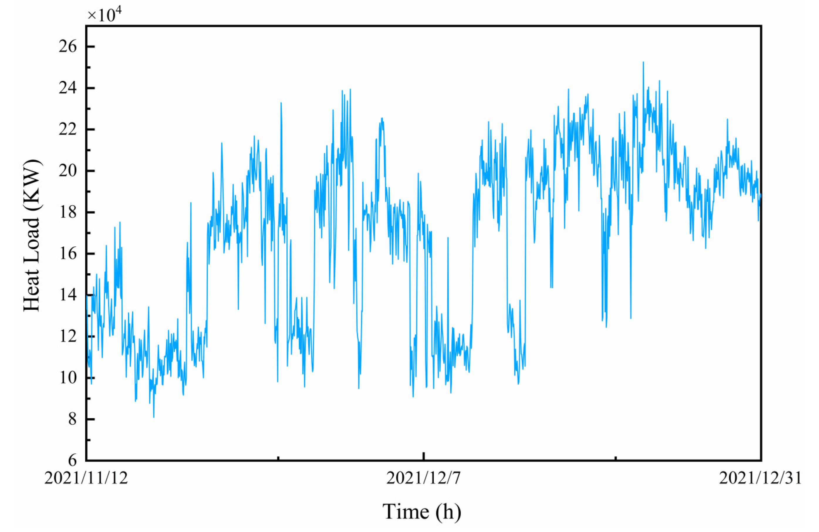
2.1. Data Sources and Composition

The data for this experiment are obtained from the real-time operational data of a heat exchange station in Changchun City. These data include 1182 sets of hourly data from 12 November to 31 December 2021. In addition, we also collected information on some variables that we could not control, such as outdoor temperature, wind speed, and solar radiation. The variation of heat load over time is shown in Figure 1.

2.2. Abnormal Data Handling

The experimental data are derived from actual operational data. Outliers may be generated during data collection due to sensor failures, manual input errors, or unusual events. In some modeling scenarios, ignoring these outliers can lead to erroneous conclusions, so it is necessary to identify these outliers and deal with them during data exploration.

Outlier detection usually includes the box plot method, 3σ principle, and simple statistical analysis. In this paper, the 3σ principle is utilized as an outlier detection method. The 3σ principle is based on equal precision repeated measures of normal distribution, which makes it challenging to match the noise or disturbance of unique data with normal distribution. The normal distribution is also known as a Gaussian distribution with a high middle, low sides, and symmetry. The probability density function of the normal distribution is $f\left(x\right)$, which is given by the following equation:

$$f\left(x\right)=\frac{1}{\sqrt{2\pi \sigma }}{e}^{-\frac{{\left(x-\mu \right)}^2}{2{\sigma }^2}}$$

(1)

The normal distribution meets the following function formula. Among them, $\sigma$ represents the standard deviation and $\mu$ represents the mean. The calculation formula is:

$$\sigma =\sqrt{\frac{1}{n-1}{\displaystyle \sum _{i=1}^n{\left(x_i-\overline{x}\right)}^2}}$$

(2)

$$\mu =\frac{1}{n}{\displaystyle \sum _{i=1}^n{x}_i}$$

(3)

The average value $\mu$ and standard deviation $\sigma$ have been calculated in the above formula. When the 3σ criterion is used, the values are almost perfectly distributed in the range ($\mu -3\sigma ,\mu +3\sigma$), with only 0.3 percent of the data falling outside this range, which can be regarded as anomalous and rejected according to the principle of small probability.

There are different processing methods for the filtered outlier: delete, treat as missing values, correct the average value, and cap method. The average value correction approach is primarily utilized in this work to handle an anomaly. The processed data are shown in Figure 2.

2.3. Data Smoothing

The experimental data are derived from real engineering projects, and encountering a significant amount of noise in the initial data is inevitable. In such cases, data smoothing methods are necessary to eliminate the noise. Various methods are available for data smoothing, including moving averages [37], exponential averages [38], and Savitzky–Golay filtering [39]. For this experiment, we are utilizing the moving average method to eliminate noise. To obtain the filtering results for the current time, each data point is replaced with the average of more than b consecutive data points from the previous period, including its data. This is a relatively straightforward method commonly employed in daily life. The calculation process can be executed as follows:

$$y_n=\frac{1}{b}{\displaystyle \sum _{i=0}^{b-1}{y}_{n-i}}$$

(4)

The equation $y_n$ represents the unprocessed data, and $b$ is the size of the sliding window. After comparison, $b$ was selected as 3 for this experiment.

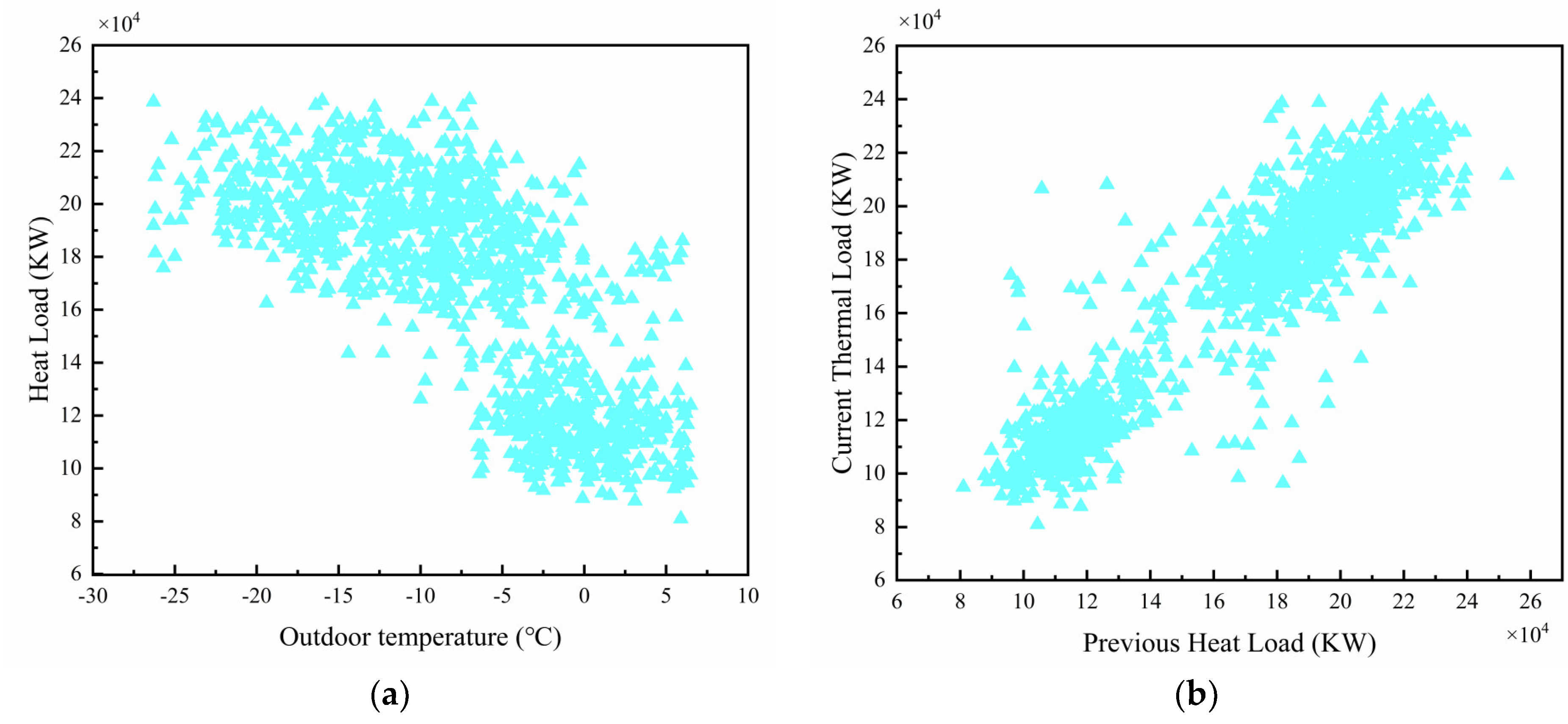
2.4. Relevance Analysis

A heating system is a complex system influenced by many factors. The main component affecting an overall heating system is outdoor meteorological factors, of which the outdoor temperature is the most important factor affecting the heat load. The heat load of a heating system is occasionally affected by internal operating parameters, such as supply pressure and return water temperature. In this experiment, several contributing factors are investigated using Pearson’s correlation coefficient analysis. The association between two variables, x (independent variable) and y (dependent variable), is measured by Pearson’s correlation coefficient. The following equation was used to calculate:

$${\rho }_{x,y}=\frac{\mathrm{cov}\left(x,y\right)}{{\sigma }_x{\sigma }_y}=\frac{E\left[\left(x-\overline{x}\right)\left(y-\overline{y}\right)\right]}{{\sigma }_x{\sigma }_y}$$

(5)

Among them, $\overline{x}$ is the average value of the independent variable $x$, $\overline{y}$ is the average value of the dependent variable $y$, ${\sigma }_x$ is the standard deviation of the independent variable $x$, and ${\sigma }_y$ is the standard deviation of the dependent variable $y$. As can be seen from the above equation, the Pearson correlation coefficient is defined as the quotient of the covariance and standard deviation between the variables. The definition ${\rho }_{x,y}$ in the above equation represents the overall correlation coefficient. After estimating the covariance and standard deviation of the variables, the Pearson correlation coefficient is obtained. Represented by $r$, as shown in the following equation:

$$r=\frac{{\displaystyle \sum _{i=1}^n\left(\frac{x_i-\overline{x}}{{\sigma }_x}\right)\left(\frac{y_i-\overline{y}}{{\sigma }_y}\right)}}{\sqrt{{\displaystyle \sum _{i=1}^n{\left(x_i-\overline{x}\right)}^2}}\sqrt{{\displaystyle \sum _{i=1}^n{\left(y_i-\overline{y}\right)}^2}}}$$

(6)

$r$ can also estimate the mean value of the standard score of ($x_i$, $y_i$) sample points to get the following expression:

$$r=\frac{1}{n-1}={\displaystyle \sum _{i=1}^n\left(\frac{x_i-\overline{x}}{{\sigma }_x}\right)}\left(\frac{y_i-\overline{y}}{{\sigma }_y}\right)$$

(7)

In the above equation, $\overline{x}$ is the average value of sample x, and $\overline{y}$ is the average value of sample y.

After analyzing the correlation between external and internal factors,

Table 1. Correlation analysis results of various influencing factors.

Classification	Factor	Correlation Coefficient
External factors	outdoor temperature	−0.746
	solar radiation	−0.062
	wind speed	−0.101
	precipitation	0.34
Internal factors	heat load at the previous moment	0.883
	water supply pressure	0.414
	return water temperature	0.539

can be obtained.

From Table 1, it can be seen that there is a significant negative correlation between outdoor temperature and heat load among the internal factors, while solar radiation, wind speed, and precipitation have relatively small effects on heat load. Among the internal factors, the heat load at the previous moment has a greater influence on the heat load, while the water supply pressure and the return water temperature have a relatively small influence on the heat load.

The scatter plots of the heat load at the current moment with the change of outdoor temperature and the previous moment are shown in Figure 3.

The scatter plot of heat load and outdoor temperature in Figure 3a shows that the heat load gradually increases as the outdoor temperature decreases. From Figure 3b, it can be seen that the heat load at the current moment increases with the increase of the heat load at the previous moment.

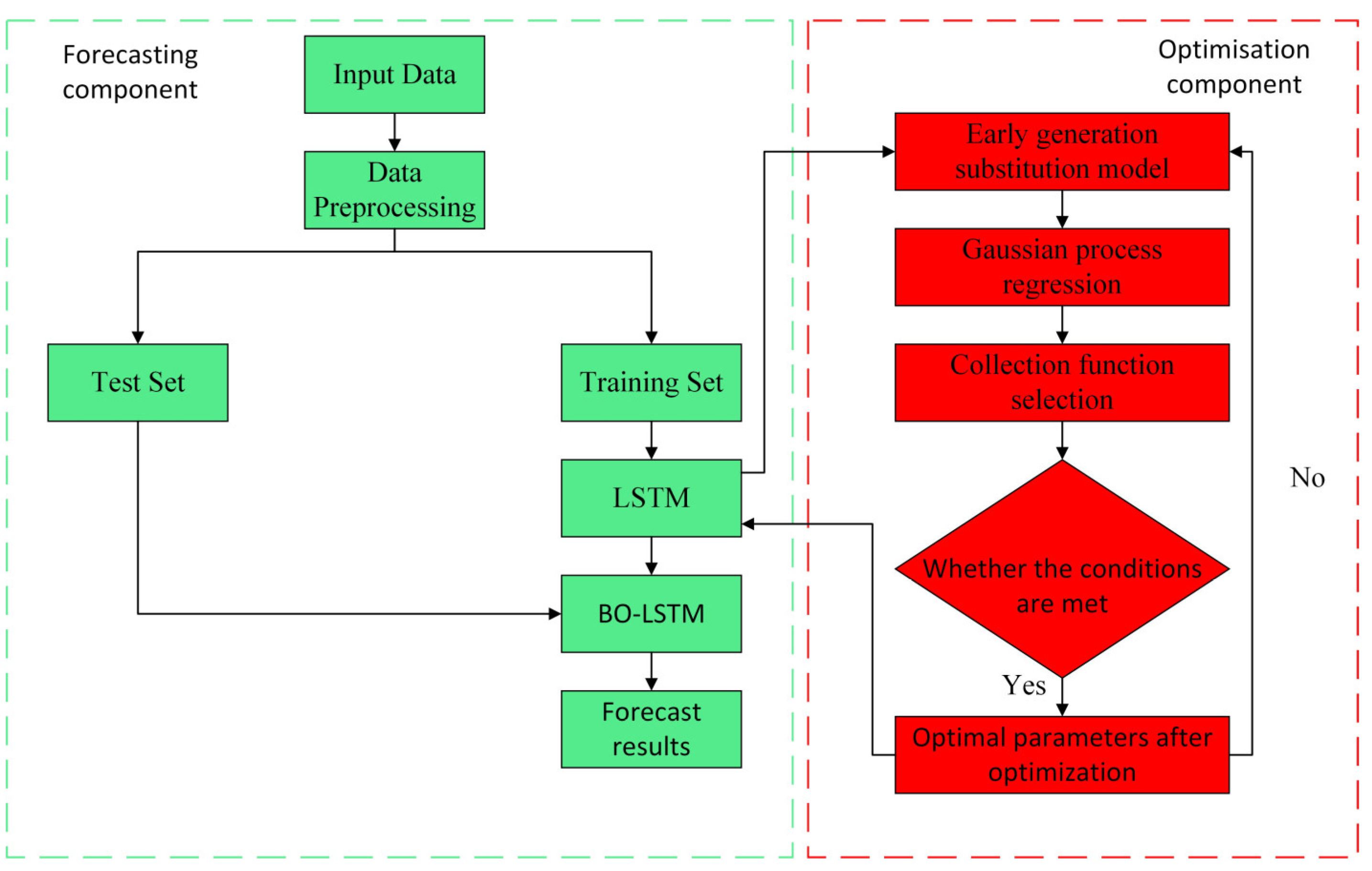
3. Forecasting Methodology

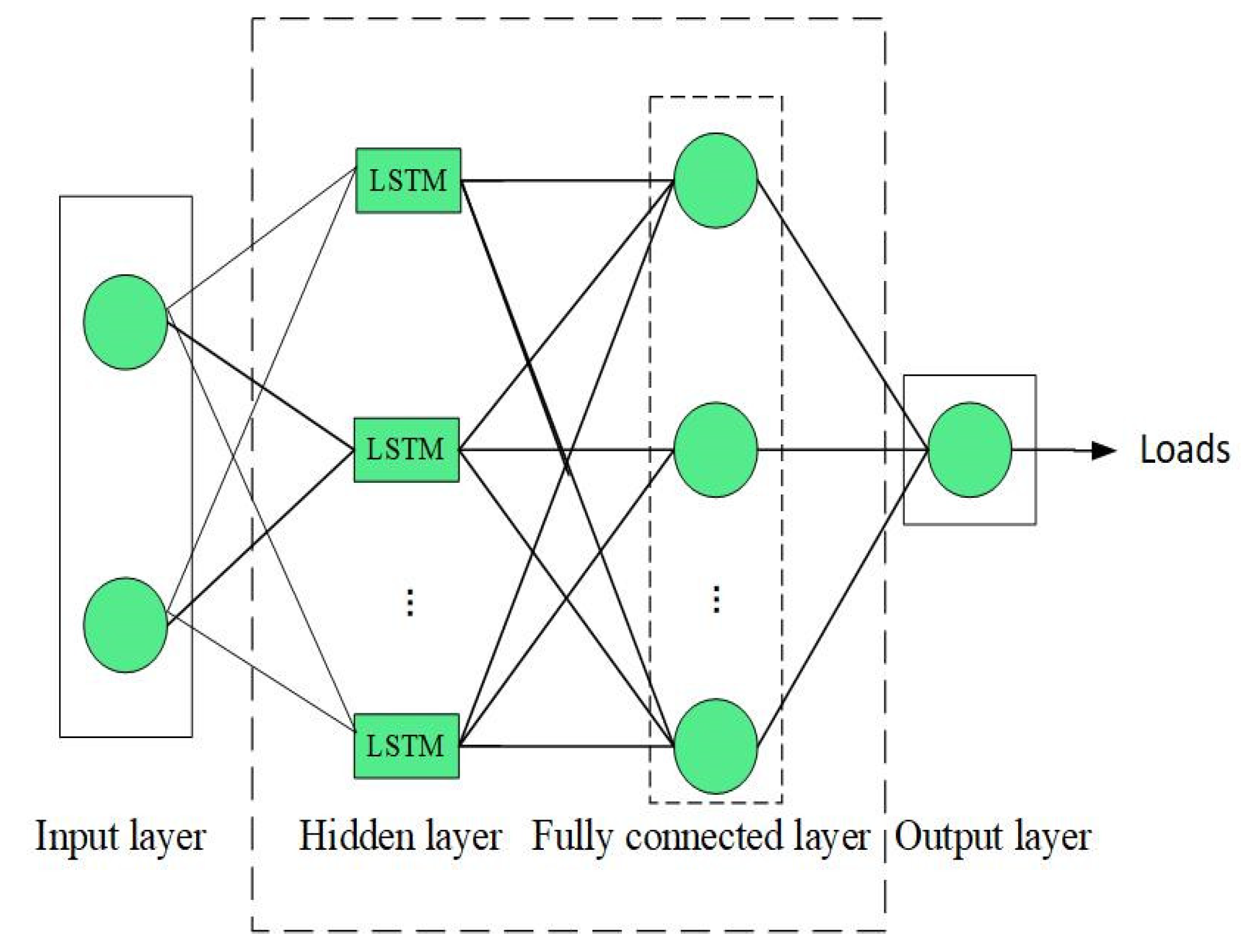
3.1. Basic Model

The data are used as time series data and were suitable for using LSTM as a prediction model. As a variation of recurrent neural network (RNN), LSTM differs from RNN in each recurrent unit. LSTM refers to three gating structures to control the transmission of information. These three gates are the input gate $i_t$, forgetting gate $f_t$, and output gate $o_t$. The input gate is used to regulate how much data have to be saved in the candidate stage. The forgot gate is used to regulate the degree to which information from the previous instant’s internal state is forgotten. The output gate regulates the information that is output from the present internal state to the external state. The following are the equations for these three gates:

$$i_t=\sigma \left(W_i{x}_t+U_i{h}_{t-1}+b_i\right)$$

(8)

$$f_t=\sigma \left(W_f{x}_t+U_f{h}_{t-1}+b_i\right)$$

(9)

$$o_t=\sigma \left(W_o{x}_t+U_o{h}_{t-1}+b_o\right)$$

(10)

where $W_f$, and $W_o$ are the weights of the input information $x$, $U_i$, $U_f$, and $U_o$ are the weights of $h_{t-1}$ at the previous time, and $b_i$, $b_f$, and $b_o$ are the biases, and the $t$ stands for time.

Wherein, $\sigma$ is the activation function, and the activation function used in this experiment is Relu, whose formula is as follows:

$$\sigma =f\left(z\right)=\left\{\begin{array}{ll}z& z>0\\ 0& z\le 0\end{array}\right.$$

(11)

It can be seen that when z is greater than 0, $f(z)$ is a linear function, but $f(z)$ is a nonlinear function in the entire definition domain. According to the function derivation rule, we can know the derivative of Relu as follows:

$$f{\left(z\right)}^{\prime }=\left\{\begin{array}{ll}1& z>0\\ 0& z\le 0\end{array}\right.$$

(12)

It can be seen that the input $z$ is positive, its derivative is 1, and the gradient does not disappear no matter how it changes. Compared with the sigmoid function and tanh function, it has a faster descent and better performance.

The established LSTM network structure diagram is presented in Figure 4.

3.2. Loss Function

The loss function plays a very important role in the backpropagation of neural networks. It is equivalent to the error. The smaller it is, the better the network will be able to solve the problem. Therefore, it is necessary to choose a suitable loss function for a more reasonable direction of the network optimization parameters.

There are many loss functions for us to use, including absolute value loss function, mean square loss function, cross-entropy loss function, etc. The mean square loss function (MSE) is used in this experiment. The expression of the mean square loss function is as follows:

$$J\left(y_i{\widehat{y}}_{\mathrm{i}}\right)=J\left(w,b\right)=\frac{1}{2m}{\displaystyle \sum _{i=1}^m{\left(y_i-{\widehat{y}}_{\mathrm{i}}\right)}^2}$$

(13)

where $y_i$ represents the true value and ${\widehat{y}}_i$ represents the predicted value.

3.3. Model Parameters

The relatively important parameters of LSTM in modeling include the number of neural network layers, the number of neural network nodes per layer, the initial learning rate, and the ridge regularization coefficient. The parameters of the experimental model are shown in

Table 2. Parameters of heat load prediction model based on LSTM.

Parameters	Value
Input layer	2
Hidden unit	50
Fully connected layer	1
Output layer	1
Initial learning rate	0.01
Learning rate decline factor	0.5
Number of iterations	10,200
Ridge regularization coefficient	0.001

.

The parameters of LSTM networks of different backgammon lengths are the same. The difference between them is the batch size, so the calculation time will also change. The unit of step size is hours (h), and the calculation time is seconds (s). The calculation time of out-of-sync length is shown in

Table 3. The calculation time of out-of-sync length.

Step Size	Value
24	204
48	178
72	314
168	255

.

3.4. Bayesian Optimization

Neural networks contain several hyperparameters, including loss function, regularisation coefficient, learning rate, and the number of structurally independent neural network layers and neurons. In traditional LSTM, these parameters are often set empirically, and it is difficult to find the most suitable parameters for the model through the empirical setting method. These hyperparameters have a great impact on the running time and prediction accuracy of the neural network, so they must be optimized. In this study, the initial learning rate, the number of nodes in the hidden layer, and the ridge regularization coefficient are chosen as the hyperparameters of the neural network and optimized using the Bayesian algorithm. Among them, ridge regularization increases the square of the weight paradigm compared with lasso regularization, which solves the problem that lasso regularization may make the model sparse. Therefore, the appropriate ridge regularization coefficient can effectively avoid overfitting.

Bayesian optimization is an optimization algorithm that optimizes a black box function by building a Gaussian process model. The core idea is to select the parameter values that are most likely to lead to optimization at each iteration based on the current Gaussian process model. Therefore, it uses Bayes’ theorem to update the prior probability distribution of the Gaussian process model and constructs the posterior probability distribution by random sampling and function evaluation. In this way, Bayesian optimization can select the next sampling point based on the information provided by the current Gaussian process model and continuously iterate to optimize the black box function. The process of LSTM Bayesian optimization is shown in Figure 5 below.

3.5. Bayesian Optimization Parameters

Similar to LSTM, the LSTM model based on Bayesian optimization also includes certain parameters in the LSTM model. The difference is that Bayesian optimization is mainly used to optimize the number of hidden layers, the ridge regularization coefficient of the LSTM, and the initial learning rate. To satisfy the optimization effect and make the optimized parameters feasible, it is necessary to set a certain range for the parameters to be optimized. In this experiment, the parameter ranges set in the four steps of 24 h, 48 h, 72 h, and 168 h are the same, as shown in

Table 4. Parameter range of Bayesian optimization.

Parameter	Range
The optimal number of hidden layer nodes	[10, 200]
The optimal initial learning rate	[1 × 10−3, 1 × 10−2]
Optimal ridge regularization coefficient	[1 × 10−5, 1 × 10−3]

.

Some of the network parameters of the Bayesian-optimized LSTM are the same as the network parameters of the LSTM built above. Bayesian optimization also uses a dual-input single-output network structure with a learning rate decline factor of 0.5. The number of Bayesian optimization iterations is 40, and the LSTM network has a total of 10,200 iterations. The difference between the two is in the optimized parameters, the running time, and the observed functional target values. The results are shown in

Table 5. Bayesian optimized parameters.

Classification	Hidden Unit	Initial Learning Rate	Time
24	40	0.002017	3911
48	199	0.0033185	4041
72	103	0.0033282	4021
168	94	0.0033598	3872

and

Table 6. Bayesian optimized parameters.

Classification	Ridge Regularization Coefficient	Observed Objective Function Value
24	0.00015493	0.077476
48	0.00010084	0.077208
72	0.00024211	0.077196
168	0.000025777	0.077409

.

4. Results of The Experiment

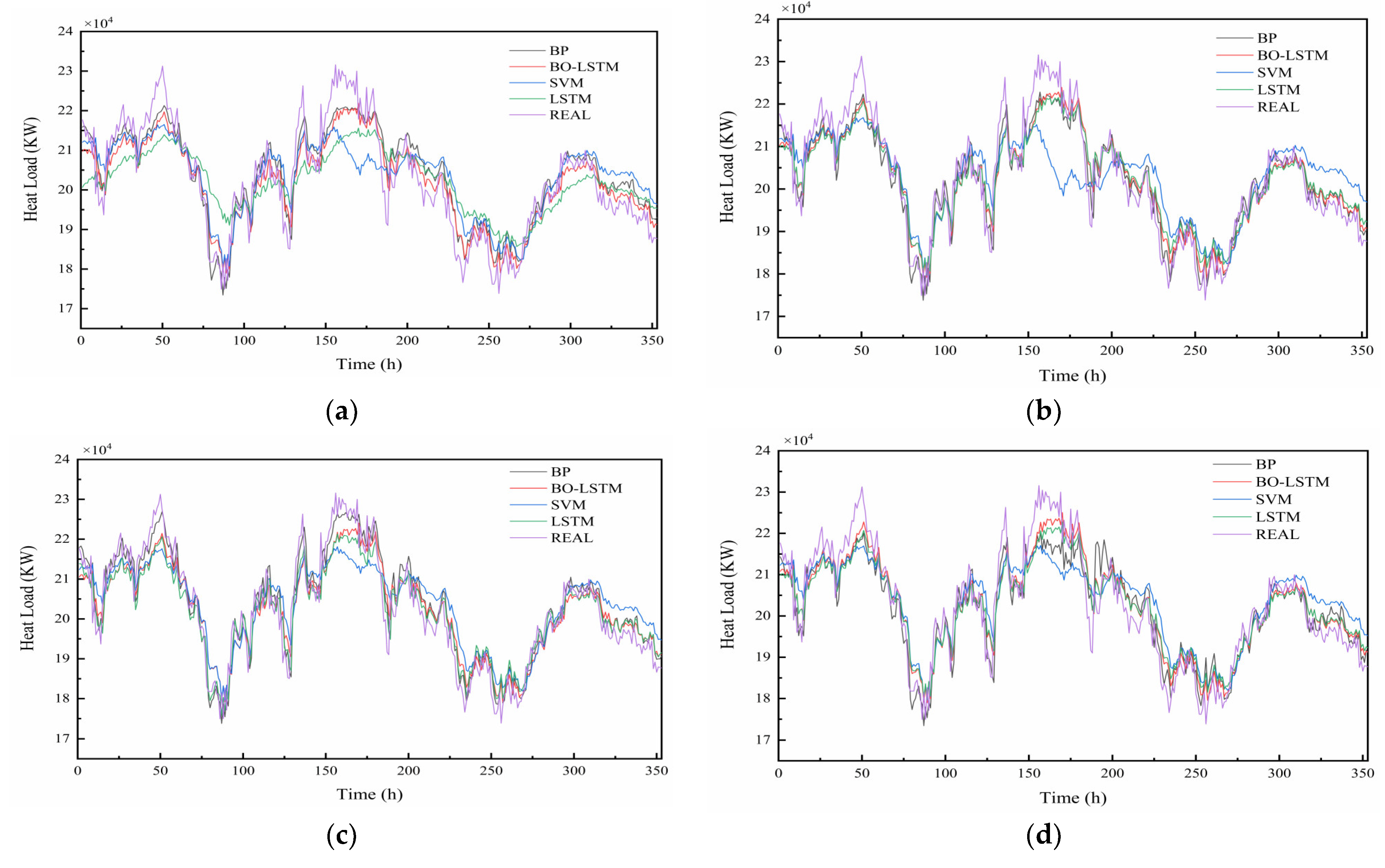
4.1. Forecast Results

The experimental data consist of multiple feature input data, including 1182 groups in total. A sufficient amount of data will ensure the fitting effect and prediction accuracy. The prediction accuracy will affect the overall energy management system as well and guide the rational use of energy. Energy production and distribution will be guided by the predicted results. In the case of heat supply, prediction results for 24 h or 48 h are usually considered. In this experiment, not only the above prediction results are considered, but also the heat loads of 72 h and 168 h are predicted, respectively. The expected results are shown in Figure 6.

From Figure 6, it can be seen that BO-LSTM has the best forecast results when making predictions. BO-LSTM can fit better in the peak and trough periods, while support vector machine (SVM) has the worst performance, followed by LSTM and BP. The different prediction steps have relatively small effects on the prediction results. When performing 24-h heat load prediction, BO-LSTM predicts less fluctuating data, which are easier to use for real heating. In reality, forecasting for longer periods may lose its regulatory significance over time. The longer the forecast, the greater the influence of stochastic factors. For example, forecasting data for more than a week may not be suitable for adjustment.

4.2. Evaluation Indicators

As a discipline that has been developed for many years, load forecasting accuracy evaluation metrics also include many methods, such as RMSE, MAE, mean square error (MSE), MAPE, symmetric mean absolute percentage error (SMAPE), R², etc. Usually, the metrics RMSE, MAE, MSE, MAPE, and SNAPE are used to evaluate the difference between the predicted and actual values. The closer the predicted results are to the actual values, the smaller the above evaluation indicators are. To observe the degree of fit, R² is used as an evaluation indicator with a value between 0 and 1. The closer the value is to 1, the better it matches the data. As an assessment indicator, R², MSE, MBE, and RMSE are utilized in this study. The equations are as follows:

$$\mathrm{RMSE}=\sqrt{\frac{1}{n}{\displaystyle \sum _{i=1}^n{\left({\widehat{y}}_i-y_i\right)}^2}}$$

(14)

$$\mathrm{MAE}=\frac{1}{n}{\displaystyle \sum _{i=1}^n\left|{\widehat{y}}_i-y_i\right|}$$

(15)

$$\mathrm{MBE}=\frac{1}{n}{\displaystyle \sum _{i=1}^n\left({\widehat{y}}_i-y_i\right)}$$

(16)

$${\mathrm{R}}^2=1-\frac{{\displaystyle {\sum }_{i=1}^n{\left(y_i-{\widehat{y}}_i\right)}^2}}{{\displaystyle {\sum }_{i=1}^n{\left(y_i-{\overline{y}}_i\right)}^2}}$$

(17)

In the formula, ${\widehat{y}}_i$ is the predicted value $y_i$ is the true value, and ${\overline{y}}_i$ is the average value of the samples $n$ is the number of samples.

The anticipated outcomes are displayed in Figure 7.

As can be seen from Figure 7, the above evaluation metrics are also different for different models. Compared with traditional LSTM, BP, and SVM, BO-LSTM shows a decrease in RMSE at all four step sizes of 24, 48, 72, and 168 h, which indicates a significant improvement in prediction accuracy. In addition, from Figure 7c, the R² of BO-LSTM is the highest for all four step lengths, indicating that the model fits best at this time. The predicted MAE and MBE decrease to different degrees at step sizes of 48, 72, and 168 h, which indicates that BO-LSTM has some advantages over LSTM.

5. Conclusions

This experiment analyzed various factors related to the heat load of a real object in long-term operation. Considering the influence of different factors, the factors with high correlation were selected as the input to the model. In terms of data pre-processing, the 3σ principle was chosen to process the data to ensure the fit. For the potential problem of data noise, the moving average method was used to smooth the data and remove the noise to make the data more reliable and easier to analyze.

For the prediction method, the LSTM optimized by the Bayesian algorithm was selected. The initial learning rate, ridge regularization coefficient, and the number of recurrent units in the hidden layer of the LSTM were optimized by using the powerful optimization ability of the Bayesian algorithm. BP, SVM, and LSTM were selected for comparison, and RMSE, R², MAE, and MBE were chosen as evaluation indexes to evaluate the prediction results of the above methods. It is easy to find that BO-LSTM had the best fitting effect through the final results. The RMSE decreased most significantly at the step size of 72 h, with a decrease of 0.15089. In other steps, the RMSE of BO-LSTM also decreased, and the other two evaluation indexes also decreased. It can be seen that the Bayesian optimized LSTM as a prediction method has a strong prediction ability and general applicability. The object of this study is not dynamic, and real-time forecasting of online dynamics is the problem that we want to solve. In addition to the above issues, there is also a problem of applying the results of hourly forecasts to actual adjustments. We believe that a real-time data acquisition and prediction platform can be built to transmit the acquired data to the prediction software via Object Linking and Embedded for Process Control (OPC) and then transmit the predicted data to the actuator for control to achieve the purpose of actual control.

References

1. Stienecker, M.; Hagemeier, A. Developing Feedforward Neural Networks as Benchmark for Load Forecasting: Methodology Presentation and Application to Hospital Heat Load Forecasting. Energies 2023, 16, 2026. [Google Scholar] [CrossRef]
2. Dahl, M.; Brun, A.; Andresen, G.B. Decision rules for economic summer-shutdown of production units in large district heating systems. Appl. Energy 2017, 208, 1128–1138. [Google Scholar] [CrossRef]
3. Huang, Y.T.; Li, C. Accurate heating, ventilation and air conditioning system load prediction for residential buildings using improved ant colony optimization and wavelet neural network. J. Build. Eng. 2021, 35, 101972. [Google Scholar] [CrossRef]
4. Yuan, J.J.; Zhou, Z.H.; Huang, K.; Han, Z.; Wang, C.D.; Lu, S.L. Analysis and evaluation of the operation data for achieving an on-demand heating consumption prediction model of district heating substation. Energy 2021, 214, 118872. [Google Scholar] [CrossRef]
5. Lu, Y.K.; Tian, Z.; Peng, P.; Niu, J.D.; Li, W.C.; Zhang, H.J. GMM clustering for heating load patterns in-depth identification and prediction model accuracy improvement of district heating system. Energy Build. 2019, 190, 49–60. [Google Scholar] [CrossRef]
6. Gao, X.; Qi, C.; Xue, G.; Song, J.; Zhang, Y.; Yu, S.-A. Forecasting the Heat Load of Residential Buildings with Heat Metering Based on CEEMDAN-SVR. Energies 2020, 13, 6079. [Google Scholar] [CrossRef]
7. Protić, M.; Shamshirband, S.; Petković, D.; Abbasi, A.; Kiah, M.L.M.; Unar, J.A.; Živković, L.; Raos, M. Forecasting of consumers heat load in district heating systems using the support vector machine with a discrete wavelet transform algorithm. Energy 2015, 87, 343–351. [Google Scholar] [CrossRef]
8. Gong, M.; Zhou, H.; Wang, Q.; Wang, S.; Yang, P. District heating systems load forecasting: A deep neural networks model based on similar day approach. Adv. Build. Energy Res. 2020, 14, 372–388. [Google Scholar] [CrossRef]
9. Sun, C.H.; Liu, Y.A.; Cao, S.S.; Gao, X.Y.; Xia, G.Q.; Qi, C.Y.; Wu, X.D. Research paper Integrated control strategy of district heating system based on load forecasting and indoor temperature measurement. Energy Rep. 2022, 8, 8124–8139. [Google Scholar] [CrossRef]
10. Dahl, M.; Brun, A.; Andresen, G.B. Using ensemble weather predictions in district heating operation and load forecasting. Appl. Energy 2017, 193, 455–465. [Google Scholar] [CrossRef]
11. Suryanarayana, G.; Lago, J.; Geysen, D.; Aleksiejuk, P.; Johansson, C. Thermal load forecasting in district heating networks using deep learning and advanced feature selection methods. Energy 2018, 157, 141–149. [Google Scholar] [CrossRef]
12. Thiangchanta, S.; Chaichana, C. The multiple linear regression models of heat load for air-conditioned room. Energy Rep. 2020, 6, 972–977. [Google Scholar] [CrossRef]
13. Wang, L.; Lee, E.W.M.; Yuen, R.K.K. Novel dynamic forecasting model for building cooling loads combining an artificial neural network and an ensemble approach. Appl. Energy 2018, 228, 1740–1753. [Google Scholar] [CrossRef]
14. Xu, H.-W.; Qin, W.; Sun, Y.-N.; Lv, Y.-L.; Zhang, J. Attention mechanism-based deep learning for heat load prediction in blast furnace ironmaking process. J. Intell. Manuf. 2023, 1–14. [Google Scholar] [CrossRef]
15. Zhou, Y.; Liang, Y.; Pan, Y.; Yuan, X.; Xie, Y.; Jia, W. A Deep-Learning-Based Meta-Modeling Workflow for Thermal Load Forecasting in Buildings: Method and a Case Study. Buildings 2022, 12, 177. [Google Scholar] [CrossRef]
16. Rusovs, D.; Jakovleva, L.; Zentins, V.; Baltputnis, K. Heat Load Numerical Prediction for District Heating System Operational Control. Latv. J. Phys. Tech. Sci. 2021, 58, 121–136. [Google Scholar] [CrossRef]
17. Jahan, I.S.; Snasel, V.; Misak, S. Intelligent Systems for Power Load Forecasting: A Study Review. Energies 2020, 13, 6105. [Google Scholar] [CrossRef]
18. Dahl, M.; Brun, A.; Kirsebom, O.S.; Andresen, G.B. Improving Short-Term Heat Load Forecasts with Calendar and Holiday Data. Energies 2018, 11, 1678. [Google Scholar] [CrossRef]
19. Zhao, J.; Shan, Y. A Fuzzy Control Strategy Using the Load Forecast for Air Conditioning System. Energies 2020, 13, 530. [Google Scholar] [CrossRef]
20. Xie, Y.; Hu, P.; Zhu, N.; Lei, F.; Xing, L.; Xu, L.; Sun, Q. A hybrid short-term load forecasting model and its application in ground source heat pump with cooling storage system. Renew. Energy 2020, 161, 1244–1259. [Google Scholar] [CrossRef]
21. Bergsteinsson, H.G.; Møller, J.K.; Nystrup, P.; Pálsson, P.; Guericke, D.; Madsen, H. Heat load forecasting using adaptive temporal hierarchies. Appl. Energy 2021, 292, 116872. [Google Scholar] [CrossRef]
22. Liu, G.; Kong, Z.; Dong, J.; Dong, X.; Jiang, Q.; Wang, K.; Li, J.; Li, C.; Wan, X. Influencing Factors, Energy Consumption, and Carbon Emission of Central Heating in China: A Supply Chain Perspective. Front. Energy Res. 2021, 9, 648857. [Google Scholar] [CrossRef]
23. Kim, J.-H.; Seong, N.-C.; Choi, W. Cooling Load Forecasting via Predictive Optimization of a Nonlinear Autoregressive Exogenous (NARX) Neural Network Model. Sustainability 2019, 11, 6535. [Google Scholar] [CrossRef]
24. Bujalski, M.; Madejski, P.; Fuzowski, K. Day-ahead heat load forecasting during the off-season in the district heating system using Generalized Additive model. Energy Build. 2023, 278, 112630. [Google Scholar] [CrossRef]
25. Castellini, A.; Bianchi, F.; Farinelli, A. Generation and interpretation of parsimonious predictive models for load forecasting in smart heating networks. Appl. Intell. 2022, 52, 9621–9637. [Google Scholar] [CrossRef]
26. Nigitz, T.; Gölles, M. A generally applicable, simple and adaptive forecasting method for the short-term heat load of consumers. Appl. Energy 2019, 241, 73–81. [Google Scholar] [CrossRef]
27. Potočnik, P.; Škerl, P.; Govekar, E. Machine-learning-based multi-step heat demand forecasting in a district heating system. Energy Build. 2021, 233, 110673. [Google Scholar] [CrossRef]
28. Bünning, F.; Heer, P.; Smith, R.S.; Lygeros, J. Improved day ahead heating demand forecasting by online correction methods. Energy Build. 2020, 211, 109821. [Google Scholar] [CrossRef]
29. Eguizabal, M.; Garay-Martinez, R.; Flores-Abascal, I. Simplified model for the short-term forecasting of heat loads in buildings. Energy Rep. 2022, 8, 79–85. [Google Scholar] [CrossRef]
30. Hofmeister, M.; Mosbach, S.; Hammacher, J.; Blum, M.; Röhrig, G.; Dörr, C.; Flegel, V.; Bhave, A.; Kraft, M. Resource-optimised generation dispatch strategy for district heating systems using dynamic hierarchical optimisation. Appl. Energy 2022, 305, 117877. [Google Scholar] [CrossRef]
31. Shepero, M.; van der Meer, D.; Munkhammar, J.; Widén, J. Residential probabilistic load forecasting: A method using Gaussian process designed for electric load data. Appl. Energy 2018, 218, 159–172. [Google Scholar] [CrossRef]
32. Kavitha, R.; Thiagarajan, C.; Priya, P.I.; Anand, A.V.; Al-Ammar, E.A.; Santhamoorthy, M.; Chandramohan, P. Improved Harris Hawks Optimization with Hybrid Deep Learning Based Heating and Cooling Load Prediction on residential buildings. Chemosphere 2022, 309, 136525. [Google Scholar] [CrossRef]
33. Chen, Z.; Chen, Y.; Xiao, T.; Wang, H.; Hou, P. A novel short-term load forecasting framework based on time-series clustering and early classification algorithm. Energy Build. 2021, 251, 111375. [Google Scholar] [CrossRef]
34. Huang, S.; Ali, N.A.M.; Shaari, N.; Noor, M.S.M. Multi-scene design analysis of integrated energy system based on feature extraction algorithm. Energy Rep. 2022, 8, 466–476. [Google Scholar] [CrossRef]
35. Gu, J.; Wang, J.; Qi, C.; Min, C.; Sundén, B. Medium-term heat load prediction for an existing residential building based on a wireless on-off control system. Energy 2018, 152, 709–718. [Google Scholar] [CrossRef]
36. Shah, P.; Choi, H.-K.; Kwon, J.S.-I. Achieving Optimal Paper Properties: A Layered Multiscale kMC and LSTM-ANN-Based Control Approach for Kraft Pulping. Processes 2023, 11, 809. [Google Scholar] [CrossRef]
37. Shibata, K.; Amemiya, T. How to Decide Window-Sizes of Smoothing Methods: A Goodness of Fit Criterion for Smoothing Oscillation Data. IEICE Trans. Electron. 2019, 102, 143–146. [Google Scholar] [CrossRef]
38. Yager, R.R. Exponential smoothing with credibility weighted observations. Inf. Sci. 2013, 252, 96–105. [Google Scholar] [CrossRef]
39. Schmid, M.; Rath, D.; Diebold, U. Why and How Savitzky–Golay Filters Should Be Replaced. ACS Meas. Sci. Au 2022, 2, 185–196. [Google Scholar] [CrossRef]
Figure 1. Heat load variation over time.
Energies 16 06234 g001
Figure 2. Treatment results of the outlier of heat load data.
Energies 16 06234 g002
Figure 3. The plot of heat load variation with influencing factors. (a) Scatter plot of outdoor temperature and heat load. (b) Scatter plot of current and previous thermal load.
Energies 16 06234 g003
Figure 4. LSTM network structure.
Energies 16 06234 g004
Figure 5. Bayesian optimization LSTM flow chart.
Energies 16 06234 g005
Figure 6. Heat load forecast results for different step lengths. (a) 24-h forecast results. (b) 48-h forecast results. (c) 72-h forecast results. (d) 168-h forecast results.
Energies 16 06234 g006
Figure 7. Error evaluation indicators of different synchronization sizes. (a) RMSE evaluation results, (b) MAE evaluation results, (c) R2 evaluation results, and (d) MBE evaluation results.
Energies 16 06234 g007