Variable Blade Inertia in State-of-the-Art Wind Turbine Structural-Dynamics Models

Abstract

This paper presents a comparison of two methods to represent variable blade inertia in two codes for aero-servo-elastic simulations of wind turbines: the nonlinear aeroelastic multi-body model HAWC2 and the nonlinear geometrically exact beam model BeamDyn for OpenFAST. The main goal is to enable these tools to simulate the dynamic behavior of a wind turbine with variable blade inertia. However, current state-of-the-art load simulation tools for wind turbines cannot simulate variable blade inertia, so the source code of these tools must be modified. The validity of the modified codes is proven based on a simple beam model. The validation shows very good agreement between the modified codes of HAWC2, BeamDyn and an analytical calculation. The add-on of variable blade inertias is applied to reduce the mechanical loads of a 5-megawatt reference wind turbine with an integrated hydraulic-pneumatic flywheel in its rotor blades.

1. Introduction

The mechanical properties of wind turbines rotor blades should not change during their operational life. However, in many cases, these properties can be changed, e.g., in smart blades [1], by using a hydraulic-pneumatic flywheel [2] or structural control (StC) [3], or as a result of atmospheric ice accretion on the blades [4]. Such changes in the mechanical properties of rotor blades affect the behavior of wind turbines significantly. To analyze the effect of variable blade mechanical properties on the dynamic behavior of a WT, rotor blades with varying mechanical properties must be first implemented in wind turbine load simulation tools. Since state-of-the-art load simulation tools for wind turbines are designed to deal with constant mechanical blade properties only, the source code of these tools must be modified to allow for variation of mechanical properties during a simulation. This variation depends on the aforementioned cases. The case investigated in this paper is a flywheel. This is due to the possibility of applying this case exactly to other cases, e.g., atmospheric ice accretion on the blades and rotor imbalance or with small modifications for the StC and smart blade cases.

The flywheel used in this paper varies the inertia of the rotor blades by moving a fluid mass between a piston accumulator near the blade root and one or more piston accumulators near the blade tip [5,6]. Consequently, the eigenfrequencies of the rotor blades and, thus, the drive train and the tower of the wind turbine can be varied by the flywheel. Additionally, the flywheel causes a driving or braking torque independent of the aerodynamic torque. This enables the rotor to be accelerated or decelerated without pitching the rotor blades [2,6,7]. To vary the rotor inertia at any arbitrary operating point of a WT, the flywheel comprises electrically-driven pumps, which support the centrifugal forces by moving the fluid from the root to the tip accumulators [2,5,6,8].

Previous investigations of the implementation of variable blade mechanical properties in aero-elastic codes of wind turbines are limited to passive StC [3,9,10,11,12,13]. The application of StC in wind turbines refers to the addition of tuned mass dampers (TMDs) to a point in the blades, nacelle, tower, or substructure. The main purpose of TMDs is to enhance damping or to generate forces to control the structural response, e.g., reduce the variability in the platform, pitch, and tower top fore-aft displacement. The proposed flywheel can, in addition to its various StC applications, also support a power system in providing different gird services [14]. Examples of flywheel’s StC applications are damping in-plane vibrations of the blades and tower, mitigating excitations from gravitation and wind shear, balancing rotors, and emergency braking [14]. The main flywheel’s grid services are power system stabilization, steadying power infeed, fast frequency response, continuous inertia provision and low voltage ride-through [14]. However, implementing the flywheel in the aero-elastic code of a wind turbine requires a simultaneous variation of the inertia of several blade nodes. Moreover, all additional forces that result from the fluid movement along the rotating blades must be applied to the correct blade nodes.

The implementation of variable blade inertia in aero-elastic codes of wind turbines has been developed in the last nine years at the Wind Energy Technology Institute (WETI) at Flensburg University of Applied Sciences, Germany. Initially, a First Eigenmodes simulation model of a wind turbine was developed to enable the design of control algorithms [15]. The model was implemented in MATLAB/Simulink and consisted of different subsystems, which described the main components of a WT. The description level of the wind turbine components was very simple to facilitate quick simulations. Consequently, an exact response of a wind turbine with variable inertia at several nodes along the blade length could not be provided by this model. To do this, a load simulation tool is required that can describe the structural dynamics of the rotor blades in more detail. One such tool is ElastoDyn, a model developed by the National Wind Technology Centre at the National Renewable Energy Laboratory (NREL), USA, which is implemented within the aeroelastic modularization framework OpenFAST [16,17]. ElastoDyn is based on the Bernoulli-Euler beam theory and describes the mechanical properties of a rotor blade in greater detail than the First Eigenmodes simulation model. Like the First Eigenmodes simulation model, ElastoDyn is free, publicly available, and well-documented. The source code of ElastoDyn has previously been modified to implement variable blade inertia [18]. Although ElastoDyn uses a simple mathematical theory based on Kane’s method [19] to establish equations of motion, the exact solutions of ElastoDyn met the needs of previous research, which also dealt with the hydraulic-pneumatic flywheel [18]. However, the method used in ElastoDyn to implement the resulting forces from the fluid movement simplifies these forces by applying a total (accumulative) torque at the hub [18]. This simplification does not consider the forces’ impact on the blade nodes, which inhibits several applications of the flywheel, e.g., damping of in-plane vibrations of blades and mitigation of excitations from gravitation and wind shear, from being simulated. Furthermore, ElastoDyn only supports beams constructed from isotropic material without mass or elastic offsets, axial or torsional DOFs and shear deformation. For these reasons, it was obvious that the method of variable blade inertia had to be implemented in a more complex structural dynamics model of wind turbine rotor blades.

Two advanced structural dynamics models, HAWC2 [20] and BeamDyn [21] were chosen to compare and validate the implementation method of variable blade inertia. Both models utilize finite beam element theory to enable a very complex and advanced modelling methods of non-linear beam structural dynamics of the blade structure. The mechanical properties of several blade cross-sections are defined in these models by tabular mass and stiffness matrices. These are used in the numerical solution of the dynamic equations during a given simulation. In addition to the extensive description of the blade’s mechanical properties, a previous comparison of HAWC2 and BeamDyn showed that both models are capable of computing accurate solutions for highly nonlinear effects [22].

The method used to implement variable blade inertia and the differences obtained by applying this method in HAWC2 and BeamDyn are presented in detail in the following section. In Section 3, the modified HAWC2 and BeamDyn models are shown to be valid for analytical calculations of three benchmarking cases of increasing complexity. An application of variable blade inertia is presented for both models in Section 4, where emergency braking is supported with the hydraulic-pneumatic flywheel.

2. Implementation of Variable Blade Inertia in HAWC2 and BeamDyn

Although the definition of beam elements in the HAWC2 and BeamDyn models differs, the mathematical description of the implementation of variable blade inertia is the same in both models. However, due to the differences in the program structure and the accessibility of the source codes of these models, two distinct implementation methods are required.

It should be noted that in this section, the matrix notation is used to denote vectorial or vectorial-like quantities. For example, vectors are denoted by an underline $\left(\underset{\_}{•}\right)$, a double underline $\left(\underset{\_}{\underset{\_}{•}}\right)$ denotes a tensor, and an overline $\left(\overline{•}\right)$ denotes a unit vector.

2.1. Superordinate Model Calculations

As discussed in the introduction, this study focuses on the variation of blade inertia resulting from a change in the global charge state of the tip accumulator, ${\gamma }_{tip}$, of a hydraulic-pneumatic flywheel. This control variable indicates whether the tip accumulators of individual blades are empty $({\gamma }_{tip}=0)$, or either partly $(0<{\gamma }_{tip}<1)$ or fully charged with fluid $({\gamma }_{tip}=1)$. Based on this variable, its derivatives and the flywheel geometry, the variable properties of the flywheel, such as fluid velocity, mass flow, and Coriolis forces, can be calculated. The equations used in this calculation are presented in Section 2.1.1 and Section 2.1.2. They are implemented identically in HAWC2 and BeamDyn.

2.1.1. Local Charge State

The flywheel in each blade has three main components: root accumulator, pipe, and tip accumulator. Each component consists of one or more elements. These elements’ geometrical and mechanical parameters are integrated into the beam element’s properties, which are defined in the input file of the model initialization. The integration comprises the definition of the start, ${\underset{\_}{R}}_{n1,i}$, and the end, ${\underset{\_}{R}}_{n2,i}$, node positions of every flywheel element, $i$, within each flywheel component, $j$. The geometrical and mechanical parameters for the tip accumulator are shown in Figure 1.

Using the start, ${\underset{\_}{R}}_{n1,i,j}$, and end, ${\underset{\_}{R}}_{n2,i,j}$, positions of the flywheel elements, the single element lengths, $l_{i,j}$, as well as the total lengths, $L_j$, of each of the three flywheel components can be determined using Equations (1) and (2).

$$l_{i,j}=\left|{\underset{\_}{R}}_{n1,i,j}-{\underset{\_}{R}}_{n2,i,j}\right|$$

(1)

$$L_j=\sum _i{l}_{i,j}$$

(2)

Equation (3) expresses the global charge state of the tip accumulator, ${\gamma }_{tip}$, as the ratio of the volume filled by a fluid, $V_{fl}$, to the total volume of the tip accumulator, $V_{tip}$.

$${\gamma }_{tip}=\frac{V_{fl}}{V_{tip}}$$

(3)

$$V_{tip}=\frac{\pi }{4}·D_{tip}^2·L_{tip}$$

(4)

$$V_{fl}=\frac{\pi }{4}·D_{tip}^2·L_{fluid\_tip}$$

(5)

where $V_{tip}$ and $V_{fl}$ in Equations (4) and (5), respectively, are determined from the diameter, $D_{tip}$, the fluid length, $L_{fluid\_tip}$, and the total length of the tip accumulator, $L_{tip}$. The global charge state of the root accumulator, ${\gamma }_{root}$, and the local charge state, ${\gamma }_{i,j}$, in each element of the flywheel components, can subsequently be derived from the global charge state of the tip accumulator, ${\gamma }_{tip}$.

The flow rate in the pipe, root and tip accumulators is constant due to the continuity and incompressibility of the fluid. Thus, the rate of change of the tip charge state, ${\dot{\gamma }}_{tip}$, can be used in Equation (6) to determine the fluid velocities, $v_{fl}$, based on the cross-sectional area, $A_j$, of the flywheel component $j$:

$$v_{fl,i,j}=\frac{V_{tip}\cdot }{A_j}$$

(6)

Similarly, the fluid acceleration, $a_{fl}$, can be calculated from from Equation (7):

$$a_{fl,i,j}=\frac{\partial v_{fl,i,j}}{\partial t}=\frac{V_{tip}\cdot {\ddot{\gamma }}_{tip}}{A_j}$$

(7)

where ${\ddot{\gamma }}_{tip}$ is the rate of change of ${\dot{\gamma }}_{tip}.$

2.1.2. Additional Forces Induced by the Flywheel

Three forces are induced by the relative motion of the fluid inside the flywheel components. The forces correspond to the exchange of the angular momentum between the blade’s stationary structure and the fluid masses. Therefore, the implementation of these forces in HAWC2 and BeamDyn is crucial for a correct representation of the operating flywheel. The three forces are graphically presented in Figure 2 and are briefly explained below:

• Coriolis forces

The radial movement of the fluid in the flywheel as the blades rotate produces Coriolis forces. Equation (8) expresses the Coriolis force, ${\underset{\_}{F}}_c$, that is applied to the center of gravitation (COG) of a considered element in terms of the cross product, $\times$, the rotational speed of the element, $\underset{\_}{\omega }$, with the fluid translational velocity, ${\underset{\_}{v}}_{fl}$, of a fluid mass, $m$, that is crossing this element.

$${\underset{\_}{F}}_c=-2\cdot m\cdot \left(\underset{\_}{\omega }\times {\underset{\_}{v}}_{fl}\right)$$

(8)

2.

Fluid inertial forces

Acceleration or deceleration of fluid in time causes fluid inertial forces. These forces balance the change of the stored momentum inside the fluid due to the change in the mass flow. Equation (9) expresses the fluid inertial forces in terms of multiplication of the fluid mass, $m$, with the fluid acceleration, ${\underset{\_}{a}}_{fl}$.

$${\underset{\_}{F}}_{fl,acc}=-m\cdot {\underset{\_}{a}}_{fl}$$

(9)

3.

Momentum flux forces

The change of flow direction or local flow speed of a fluid due to a sudden change in the cross-sectional area causes hydraulic reaction forces to balance the difference in the transported momentum between the inlet and the outlet of a control volume. These forces are called momentum flux forces, ${\underset{\_}{F}}_{fl,mom,i}$, and shown in Equation (10) as a difference in the hydraulic reaction forces between two neighbors elements.

$${\underset{\_}{F}}_{fl,mom,i}={\left({\dot{m}}_{out}\cdot {\underset{\_}{v}}_{fl}\right)}_{i-1}-{\left({\dot{m}}_{in}\cdot {\underset{\_}{v}}_{fl}\right)}_i$$

(10)

where ${\left({\dot{m}}_{out}\right)}_{i-1}$ is the fluid mass flow at the outlet of the previous element, $i-1$, and ${\left({\dot{m}}_{in}\cdot {\underset{\_}{v}}_{fl}\right)}_i$ is the fluid mass flow at the inlet of the considered element, $i$.

If these three forces are treated correctly within the HAWC2 and BeamDyn models, the conservation law of momentum and angular momentum of a wind turbine with a flywheel in its rotor should still hold.

Other forces, which are related to the stationary effects of the additional fluid masses inside the blade, are independent of the translational motion of the fluid. These forces, e.g., gravitational, centrifugal, gyroscopic, and inertial forces from fluid without relative motion in any arbitrary direction, are handled inside the original implementation methods in HAWC2 and BeamDyn.

2.2. Implementation of Variable Blade Inertia in HAWC2

HAWC2 is a state-of-the-art aeroelastic code developed by DTU [20] and used in academia and industry. The structural dynamics model of HAWC2 is based on the flexible multibody approach using interconnected bodies consisting of Timoshenko finite-element beams. The body motions are described by a method called ‘floating frame of reference’ [20], described in [23]. The equations of motion (EOM) use a redundant set of coordinates consisting of the body reference motion DOFs, the relative elastic motion DOFs and a set of algebraic constraints [20].

Since HAWC2 is a closed source, users cannot create more complex models by changing the source code. For this reason, the HAWC2 developers created a DLL programming interface called the External System interface [24]. This allows the user to define general second-order dynamic equations and general algebraic constraints outside the HAWC2 core in user-written DLL files. The added external DOFs defined in the DLL files are solved as additional generalized coordinates with the HAWC2 coordinates in a common equation system [25]. This approach has previously been applied to simulate a planetary gearbox and dynamic mooring lines along with the HAWC2 beam models [24] and was chosen in the present work as the basis for developing a flywheel model extension with variable inertia.

The general second-order differential-algebraic dynamic equation system of the External System’s DOFs and external constraints in a user-written DLL takes the form of Equations (11) and (12) [24]:

$$\underset{\_}{\underset{\_}{M}}\cdot \underset{\_}{\ddot{q}}+\underset{\_}{\underset{\_}{C}}\cdot \dot{\underset{\_}{q}}+\underset{\_}{\underset{\_}{K}}\cdot \underset{\_}{q}-\underset{\_}{F}+{\underset{\_}{\underset{\_}{G}}}_e\cdot \underset{\_}{\lambda }=\underset{\_}{0}$$

(11)

and

$$\underset{\_}{g}=\underset{\_}{0}$$

(12)

where $\underset{\_}{\underset{\_}{M}},$ $\underset{\_}{\underset{\_}{C}}$ and $\underset{\_}{\underset{\_}{K}}$ are the External System’s mass, damping and stiffness matrices, respectively. The generalized acceleration, velocity, and coordinates (consisting of the External System’s DOFs) are represented by $\underset{\_}{\ddot{q}}$, $\dot{\underset{\_}{q}}$ and $\underset{\_}{q}$, respectively. $\underset{\_}{F}$ is the vector of the sum of generalized external forces. The constraint Jacobian matrix, ${\underset{\_}{\underset{\_}{G}}}_e$, and the vector of Lagrange Multipliers, $\underset{\_}{\lambda }$, are associated with the algebraic constraint equations $\underset{\_}{g}$. ${\underset{\_}{\underset{\_}{G}}}_e$ and $\underset{\_}{\lambda }$ represent constraint reaction forces and transfer loads between the External System and HAWC2 bodies.

The HAWC2 solver solves the set of Equations (11) and (12) together with the internal equations of the multibody system with respect to time. This ensures a tight coupling of the External Systems’ dynamic models with the original multibody system.

2.2.1. Model Idea and Assumptions

The main idea of the flywheel implementation in HAWC2 is based on the fact that variable inertia can be added via External System, which uses Equations (11) and (12) to describe the physical properties.

The overall implementation concept consists of the following ideas and assumptions:

• By applying fluid dynamics theory using the Eulerian description, the fluid in the flywheel can be subdivided into several elements forming control volumes (CV), which are fixed relative to the blade beams. Each element is then modeled as an External System.
• The effects of the contained (static) fluid mass in the CV, which can vary over time, can be addressed by changing the mass matrices $\underset{\_}{\underset{\_}{M}}$ and forces $\underset{\_}{F}$ associated with the contained mass.
• The effects associated with the change of the fluid mass (cf. Section 2.1.2) must be added as external forces $\underset{\_}{F}$ acting on the CV. These effects are otherwise not covered by elements with constant properties, and they are crucial to fulfil the conservation law of momentum.
• To simplify the momentum balance and calculation of mass matrices, a ‘lumping’ approach was chosen. This means that the flexible pipes and accumulators are approximated as piecewise rigid segments, and the deformation of a single element as the blade bends is neglected. Thus, each element is of constant size and not deformable, implying it can be reduced to a rigid body. The bending of the pipes and accumulators with blade bending is modeled as relative rotation between the rigid elements rather than modelling deformations. This also implies that the stiffness matrix $\underset{\_}{\underset{\_}{K}}$ and the damping matrix $\underset{\_}{\underset{\_}{C}}$ in Equation (11) are 0, and are no DOFs needed to model deformations.
• Because the constant-sized CVs are chosen to be cylindrical and straight, stream tube theory can be applied to model the forces from fluid dynamics. Fluid is assumed to change its flow direction only at the connection between two adjacent flywheel elements. From these assumptions, it follows that Equations (8)–(10) are sufficient to satisfy the conservation of momentum in the flywheel.

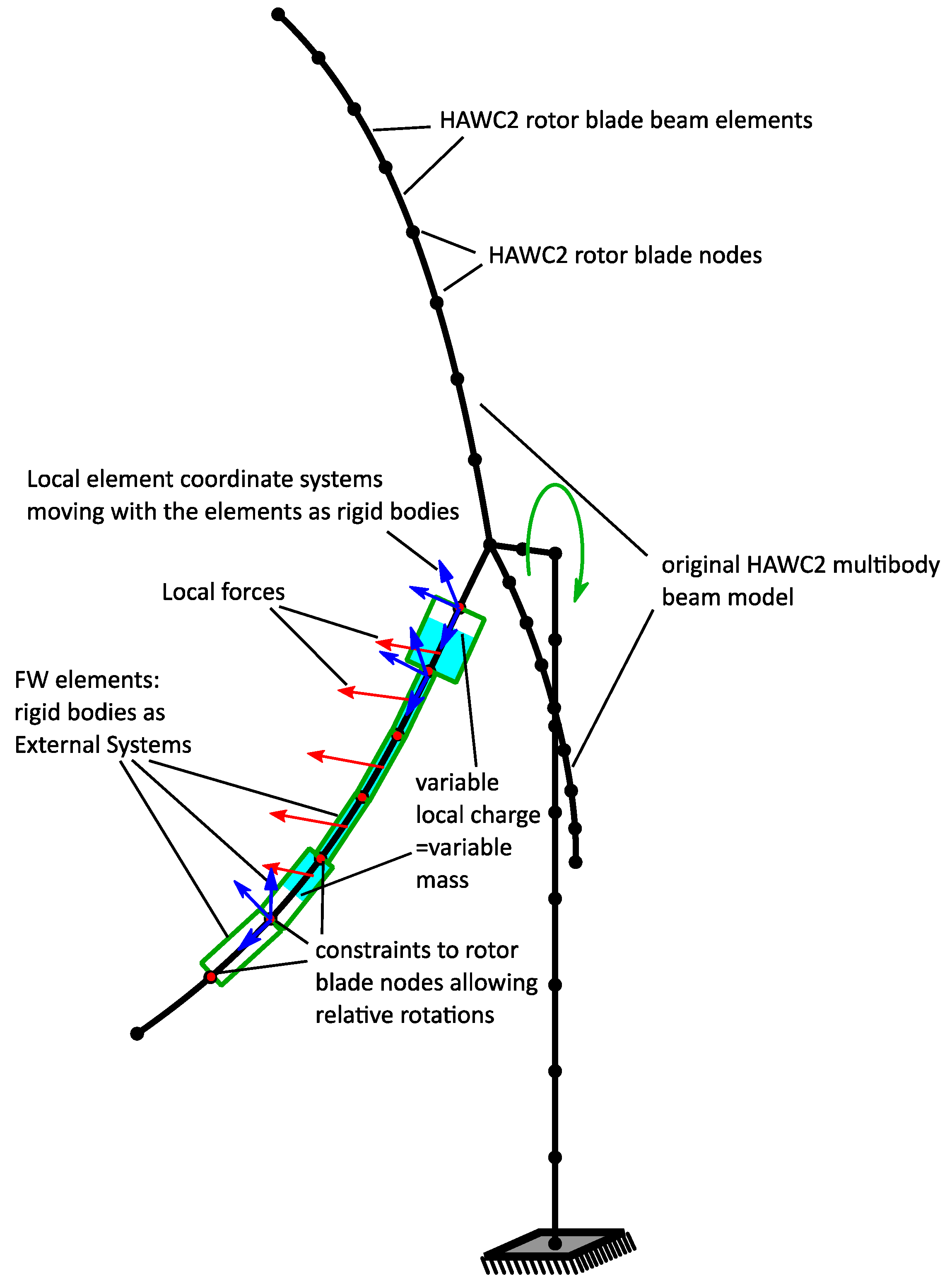
The implementation concept for the flywheel is shown schematically in Figure 3 for a simple HAWC2 simulation model with flywheel elements as External Systems at one blade. This concept uses DLLs developed by AEROVIDE GmbH. The flywheel can be independently controlled by external control software. The only control signals required during simulation are the global charge state of each blade and its derivatives.

2.2.2. Equations of Motion and the Definition of DOFs

As each flywheel element is assumed to represent a rigid body in 3D space, the Newton-Euler equations are suitable [23] to model their motion and were used in the implementation of the flywheel model. There are six Newton-Euler equations, (three for translation and three for rotation), which can be seen in Equation (13) as a specific form of the general dynamic equations of the External System’s DOFs.

$$\underset{\_}{\underset{\_}{M}}\cdot \left(\begin{array}{c}\ddot{\underset{\_}{R}}\\ \dot{\underset{\_}{\omega }}\end{array}\right)=\left(\begin{array}{c}{\underset{\_}{F}}_v\\ {\underset{\_}{M}}_v\end{array}\right)+\left(\begin{array}{c}{\underset{\_}{F}}_g\\ {\underset{\_}{M}}_g\end{array}\right)+\left(\begin{array}{c}{\underset{\_}{F}}_c\\ {\underset{\_}{M}}_c\end{array}\right)+\left(\begin{array}{c}{\underset{\_}{F}}_{fl}\\ \underset{\_}{0}\end{array}\right)-{\underset{\_}{\underset{\_}{G}}}_e\cdot \underset{\_}{\lambda }$$

(13)

where the newly introduced variables in the equation are defined as follows. ${\underset{\_}{F}}_g$ is the gravitational force. ${\underset{\_}{F}}_c$ is the Coriolis force from Equation (8). ${\underset{\_}{F}}_{fl}$ is the sum of the fluid inertial force and the moment force at the element, see Equations (9) and (10). ${\underset{\_}{M}}_g$ and ${\underset{\_}{M}}_c$ the offset moments of the gravitational force and the Coriolis force, respectively, caused by the variable COG offset to the element’s origin. ${\underset{\_}{F}}_v$ and ${\underset{\_}{M}}_v$ are the centrifugal and gyroscopic force and moment terms, respectively, which occur in the Newton-Euler equations [23]. The vector $\underset{\_}{R}$ denotes the element origin’s position and is discussed further in the following paragraph.

The Newton-Euler equations are characterized by a specific choice of coordinates for the description of rigid body motion with geometric meanings: The three translational motion DOFs are described by the element origin’s position vector $\underset{\_}{R}$ and the acceleration $\ddot{\underset{\_}{R}}$, measured in global HAWC2 coordinates. The global HAWC2 coordinates are fixed in space at the ground and thus serve as the inertial reference frame (see HAWC2 manual [20]). The three rotational DOFs are described by the local angular velocity vector $\underset{\_}{\omega }$ and the local angular acceleration $\dot{\underset{\_}{\omega }}$, measured around the element’s axes. These axes are rigidly fixed to the element and thus always rotate with the element relative to the global HAWC2 coordinates.

As the integrated local rotation coordinates, see Equation (14), do not contain unique 3D orientation information of the local element’s axes [23], the rotations need to be calculated in another way to define the orientation of the local element’s axes. To do so, Euler parameters, $\theta ,$ are used as extra rotation coordinates, as the time derivates of the Euler parameters, $\dot{\theta }$, are related to the local angular velocity vector $\underset{\_}{\omega }$ [23]. During each HAWC2 solver update of the 6 External System DOFs ($\underset{\_}{R}$, $\underset{\_}{\dot{R}}$, $\underset{\_}{\ddot{R}}$, $\underset{\_}{\phi }$, $\underset{\_}{\omega }$, and $\underset{\_}{\ddot{\omega }}$), the associated Euler parameters can be updated by integration, accordingly. The Euler parameters can then be transformed into an element rotation matrix, $\underset{\_}{\underset{\_}{A},}$ for each time step. The rotation matrix $\underset{\_}{\underset{\_}{A}}$ finally defines the orientation of the local element’s axes with respect to the global HAWC2 coordinate axes [23] (see Figure 3) and is therefore required to transform forces and moments from the local element coordinates to the global HAWC2 coordinates and vice versa.

$$\underset{\_}{\phi }=\int \underset{\_}{\omega }\mathrm{d}t$$

(14)

The element origin position described by $\underset{\_}{R}$ is chosen to be equal to the element’s start node position ${\underset{\_}{R}}_{n1,i,j}$. Thus, the origin position and the variable COG position are decoupled. This is a requirement of model assumption (a.), see Section 2.2.1. The local axes relative to the element are defined with the z-axis pointing from the origin to the element’s end node position, ${\underset{\_}{R}}_{n2,i,j}$. Consequently, the z-axis always points in the direction of the element’s length axis. The x- and y-axis orientations are arbitrarily chosen to be radial to the element, forming a right-handed Cartesian coordinate system (see Figure 4).

The mass matrix of a flywheel element is continuously updated via the superordinate model calculations as the charge state varies. Consequently, the mass matrix in Equation (15) takes the form partitioned into translational and rotational DOFs:

$$\underset{\_}{\underset{\_}{M}}=\left(\begin{array}{cc}\underset{\_}{\underset{\_}{I_3}}\cdot m& -\underset{\_}{\underset{\_}{A}}\cdot {\underset{\_}{\underset{\_}{\tilde{u}}}}_g\cdot m\\ -\underset{\_}{\underset{\_}{A}}\cdot {\underset{\_}{\underset{\_}{\tilde{u}}}}_g\cdot m& {\underset{\_}{\underset{\_}{J}}}_g-m\cdot {\underset{\_}{\underset{\_}{\tilde{u}}}}_g\cdot {\underset{\_}{\underset{\_}{\tilde{u}}}}_g\end{array}\right)$$

(15)

where $\underset{\_}{\underset{\_}{I_3}}$ is the $3\times 3$ identity matrix and $m$ is the contained mass. ${\underset{\_}{u}}_g=\left(\begin{array}{c}0\\ 0\\ z_g\end{array}\right)$ is the center of gravity measured in local element coordinates and ${\underset{\_}{\tilde{u}}}_g=\left(\begin{array}{ccc}0& -z_g& 0\\ z_g& 0& 0\\ 0& 0& 0\end{array}\right)$ is the skew-symmetric matrix associated with ${\underset{\_}{u}}_g$. Last, $\underset{\_}{\underset{\_}{J_g}}$ is the inertia tensor measured in local element coordinates referred to as the center of gravity.

In the calculation of the mass properties of the elements, they are considered to be solid fluid cylinders with the calculated height of the fluid in the element and the diameter of the element.

2.2.3. Constraints

Without constraints, the Newton-Euler equations would allow the flywheel elements to move freely in the 3D space. As the flywheel elements represent additional masses inside the rotor blades, the constraints are formulated such that flywheel elements are always moving with the rotor blade. The start and end nodes of adjacent elements are always linked like a chain, even under blade pre-bending and bending. This can be achieved by constraining both the start and the end nodes of each element, ${\underset{\_}{R}}_{n1,i,j}$ and ${\underset{\_}{R}}_{n2,i,j}$, to nearby nodes of the rotor blade body and allowing rotations of the element relative to the rotor blade nodes. One disadvantage of this approach is that a non-tree-like structure is created because of constraints at two positions on each element. The non-tree-like structure is commonly called a ‘kinematic loop’ [25] and causes increased stiffness of the rotor blade when statically overdetermined constraints are used.

So that the kinematic loop does not change blade stiffness or impose numerical problems, the constraint equations of the flywheel elements are chosen so that each flywheel motion DOF is restricted only once. As in applied mechanics, this is achieved in the model by using algebraic constraint equations as a statically-determined simple support for the flywheel element. The constraints describe a 3-dimensional fixed-floating bearing setup for each flywheel element. Using the fixed-free bearing setup does not lead to constraint reaction forces at the bearings by bending, axial elongation or torsion between two rotor blade nodes, and thus, there is no influence on the stiffness.

The start and end node positions of the elements, ${\underset{\_}{R}}_{n1,i,j}$ and ${\underset{\_}{R}}_{n2,i,j}$ respectively, can be chosen to coincide with the nodes of the rotor blade body. However, placing the flywheel elements near the rotor blade nodes with a radial offset is also possible. This might be desired, e.g., to let the flywheel element’s length axis coincide with the blade’s mass axis or to follow the real geometric position of the flywheel component. Both may have an offset to the axis formed by the blade nodes.

The constraint setup and the allowed relative motions are visualized in Figure 5. The required constraint equations can be taken from multibody simulation and robotics textbooks (e.g., [23]).

The fixed bearing restricts relative translational motion between the flywheel element’s start node and a rotor blade node, and additionally rotation around the length axis. The floating bearing only restricts relative translational motion between the flywheel element’s end node and a rotor blade node radial to the element’s length axis.

2.3. Implementation of Variable Beam Inertia in BeamDyn

BeamDyn is a nonlinear beam finite element model for simulating slender structures created by the National Wind Technology Center at the National Renewable Energy Laboratory (NREL), USA [21]. The model is used by the FAST aero-hydro-servo-elastic wind turbine multi-physics engineering tool to model blade structural dynamics. BeamDyn uses geometrically exact beam theory (GEBT) [26]. A spatial discretization for the GEBT beam equations is accomplished with Legendre spectral finite elements (LSFEs) [27]. The combination of GEBT and LSFEs enables BeamDyn to model long, flexible, composite wind turbine blades with a single high-order element [21].

BeamDyn is open-source software, which can be used to model the flywheel directly in its source code. The modelling concept is based on a variable change of the cross-sectional mass matrices during a given simulation and the addition of the forces induced by the flywheel to the external distributed forces, e.g., aerodynamic forces, hydrodynamic forces, and user-defined loads in the BeamDyn input file.

2.3.1. Modification of the Mass Matrix

A blade input file defines the mechanical parameters of the blade in the form of cross-sectional mass and stiffness matrices at various stations along a blade and six damping coefficients for the whole blade. These parameters are defined as constants in the initialization source code of BeamDyn. Hence, these parameters, e.g., the mass matrix, $\underset{\_}{\underset{\_}{\mathcal{M}}}$, in Equation (16), do not change their values during a simulation. The source code of BeamDyn is modified so the cross-sectional mass matrix parameters are changed from time-invariant parameters to time-variant variables. This modification takes place at the beginning of the dynamic solution of BeamDyn to ensure that all forces associated with the additional fluid masses are updated correctly.

The original, $\underset{\_}{\underset{\_}{\mathcal{M}}}$, and the modified, ${\underset{\_}{\underset{\_}{\mathcal{M}}}}^{\ast }$, sectional mass matrices are given by Equations (16) and (17), respectively.

$$\underset{\_}{\underset{\_}{\mathcal{M}}}=\left[\begin{array}{cccccc}m& 0& 0& 0& 0& -m{Y}_{cm}\\ 0& m& 0& 0& 0& m{X}_{cm}\\ 0& 0& m& m{Y}_{cm}& -m{X}_{cm}& 0\\ 0& 0& m{Y}_{cm}& i_{Edg}& {-i}_{cp}& 0\\ 0& 0& -m{X}_{cm}& {-i}_{cp}& i_{Flp}& 0\\ -m{Y}_{cm}& m{X}_{cm}& 0& 0& 0& i_{plr}\end{array}\right]$$

(16)

$${\underset{\_}{\underset{\_}{\mathcal{M}}}}^{\ast }=\left[\begin{array}{cccccc}m+m_{fluid}& 0& 0& 0& 0& -m Y_{cm}\\ 0& m+m_{fluid}& 0& 0& 0& m X_{cm}\\ 0& 0& m+m_{fluid}& m Y_{cm}& -m X_{cm}& 0\\ 0& 0& m Y_{cm}& i_{Edg}+i_{fluid}& {-i}_{cp}& 0\\ 0& 0& -m X_{cm}& {-i}_{cp}& i_{Flp}+i_{fluid}& 0\\ -m Y_{cm}& m X_{cm}& 0& 0& 0& i_{plr}+2i_{fluid}\end{array}\right]$$

(17)

where $m$ and $m_{fluid}$ are the blade structural and the fluid mass density per unit span, respectively. The local coordinates of the sectional center of mass are expressed by $X_{cm}$ and $Y_{cm}$. $i_{Edg}$, $i_{Flp}$ and $i_{Fluid}$ are the edge, flap, and fluid mass moments of inertia per unit span, respectively. $i_{cp}$ is the sectional cross-product of inertia per unit span; and $i_{plr}$ is the polar moment of inertia per unit span.

2.3.2. Additional External Distributed Forces

Externally applied loads, including uniformly distributed, point, and tip-concentrated forces, can be defined in the input file of BeamDyn. By customizing the source code, BeamDyn can handle more complex external force cases, such as those induced by the flywheel. Hence, the three aforementioned types of forces are in Section 2.2.2. (Coriolis forces, fluid inertial forces and momentum flux forces) They are defined as distributed forces in the dynamic solution subroutines, which are applied at every time step. $\underset{\_}{{\mathcal{F}}_{add}}$, shown in Equation (18), is the addition of the x, y, and z components of the distributed Coriolis forces, $\underset{\_}{{\mathcal{F}}_c}$, the distributed fluid inertial forces, $\underset{\_}{{\mathcal{F}}_{fl\_acc}}$, and the momentum flux forces, $\underset{\_}{{\mathcal{F}}_{fl\_mom}}$, in the local coordinates.

$$\underset{\_}{{\mathcal{F}}_{add}}=\underset{\_}{{\mathcal{F}}_c}+\underset{\_}{{\mathcal{F}}_{fl\_acc}}+\underset{\_}{{\mathcal{F}}_{fl\_mom}}$$

(18)

Since, the source code allows for the input of applied distributed loads in the global coordinate system, the additional forces, $\underset{\_}{{\mathcal{F}}_{add}}$, must be transformed to the global coordinate system. This transformation is shown in Equation (19).

$$\underset{\_}{{\mathcal{F}}_{add}^G}=\underset{\_}{\underset{\_}{\mathcal{R}}}·\underset{\_}{{\mathcal{F}}_{add}}$$

(19)

where $\underset{\_}{{\mathcal{F}}_{add}^G}$ represents the additional forces in the global coordinate system and $\underset{\_}{\underset{\_}{\mathcal{R}}}$ is the rotation tensor expressed in terms of Wiener-Milenković parameters [28,29]. The additional forces, $\underset{\_}{{\mathcal{F}}_{add}^G}$ can be added to the applied distributed loads.

FAST_SFunc is used to input the global charge state signals and their derivatives in the source code of BeamDyn. FAST_SFunc is a FAST interface to Simulink, implemented as a Level-2 S-Function. The Level-2 S-Function is a Simulink block written in C, and it calls a DLL of FAST routines written in Fortran [30,31]. This interface allows external modules, such as the control and auxiliary systems of the hydraulic-pneumatic flywheel, to be implemented in Simulink. During a simulation, the flywheel can be simulated together with the nonlinear aero-elastic tool OpenFAST [32]. However, to pass the flywheel signals through FAST_SFunc, the source code of the OpenFAST glue code needs to be modified. This is because FAST_SFunc is set up to receive only the control signals from the OpenFAST standard modules, such as generator torque control, nacelle yaw control, pitch control, and high-speed shaft brake.

3. Validation

In this section, three benchmarking cases are discussed. The complexity of the cases increases gradually. The main objective of these cases is to validate the method used in HAWC2 and BeamDyn to implement variable blade inertia. The validation is based on the proof of the physical laws of the equilibrium conditions and the conservation of angular momentum. The physical laws are analytically computed and compared with simulation results from the modified HAWC2 and BeamDyn models in all three cases.

It needs to be mentioned here that BeamDyn standalone is only set up to define a constant angular rotation of the beam root about its rotation axis. Complex root motions such as those treated in Cases 2 and 3 can only be simulated when BeamDyn is used within the wind turbine simulation tool OpenFAST. However, running BeamDyn within OpenFAST requires the specification of some physically realistic generator rotational inertia, even when the generator model is deactivated. Hence, a generator inertia of 115,926 kg-m² is used in the simulation and the analytical calculation.

The HAWC2 models for the benchmarking cases are defined in accordance with the demands from BeamDyn within OpenFAST. Hence the same beam parameters and additional generator rotational inertia are used.

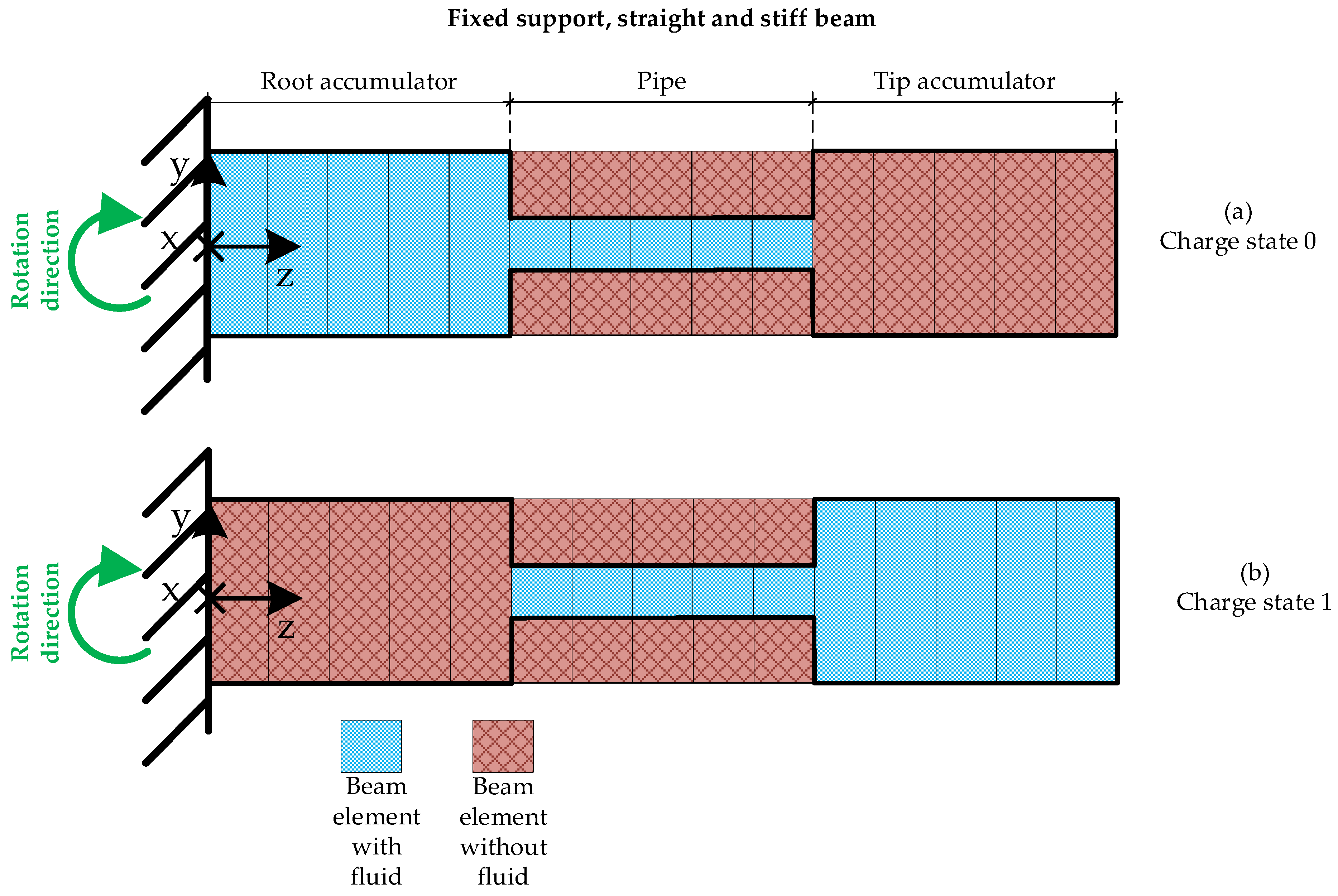
3.1. Case 1: Fixed Rotational Speed of a Fixed, Supported, Straight and Stiff Beam

Case 1 concerns the reaction forces and moments of a fixed supported beam subjected at its fixed end to a constant rotational speed around the x axis and axial fluid movement along the z axis.

The beam is straight and discretized in 15 elements. The length of each element is 1 m. Three hydraulic components are integrated into the beam: pipe, root, and tip accumulators. Each component has five elements. The total fluid mass moved between the root and the tip accumulators equals 500 kg. A schematic drawing of the beam in charge states 0 and 1 is shown in Figure 6a,b, respectively.

When the charge state equals 0, the root accumulator is full, and the tip accumulator is empty. Conversely, the root accumulator is empty, and the tip accumulator is full when the charge state equals 1. The charge state, therefore, varies between 0 and 1 as the fluid moves between the root and the tip accumulators.

The beam’s input cross-sectional mass and stiffness parameters are presented in

Table 1. Cross-sectional mechanical properties of the straight and stiff beam.

Beam Elementmass Density	Flap and Edge Mass Moments of Inertia per Unit Span	Flap Stiffness	Edge Stiffness	Flap Shear Stiffness	Edge Shear Stiffness	Torsional Stiffness
kg/m	kg·m	N∙m2	N∙m2	N∙m2	N∙m2	N∙m2
50	50	1.00 × 1010	1.00 × 1010	5.00 × 108	5.00 × 108	1.00 × 109

. In Case 1 and later in Case 2, the beam stiffnesses are set to very high values to prevent the beam from bending. This keeps the local coordinates of the beam elements synchronized with the root coordinates of the beam at the fixed end coordinates of the beam and simplifies the analytical calculation of the reaction forces and moments.

For Case 1, the simulation scenario presented in Figure 7 sets the rotational speed to a constant value of 10 rpm. The charge state rises from 0 to 1 between 10 s and 50 s and remains constant till 60 s. Between 60 s and 100 s the charge state is reduced from 1 to zero and remains at 0 until the end of the simulation. Reaction forces and moments result from the fluid movement. The x, y and z components of these forces and moments are analytically calculated and compared with the corresponding simulation results from HAWC2 and BeamDyn. The comparisons in Figure 7 show a very good agreement between the analytical and the simulated results of all components. The increase/decrease of the y component of the reaction force is due to the Coriolis forces that result from the change in the charge state. Hence, a reaction moment around the x axis results from these Coriolis forces. The z component of the reaction force illustrates the sum of the centrifugal and fluid inertial forces. The variation in the centrifugal forces results from the change in the COG of the beam due to the fluid motion. The fluid inertial forces (Equation (9)) can be seen, when the fluid accelerates, e.g., from 10 to 11 s, or deaccelerates, e.g., from 50 to 51 s.

3.2. Case 2: A Pinned-Supported, Straight and Stiff Beam

The purpose of Case 2 is to prove the conservation of angular momentum when the beam inertia changes in a free rotational system. Case 2 uses the same beam used in Case 1, pinned supported. See Figure 8. This support enables the beam to rotate freely and prevents translational movement at the supported end. Since the angular momentum in a free rotational system remains constant, the rotational speed of the beam decreases when the beam inertia increases, and vice versa. On this basis, the variable rotational speed of the beam can be analytically calculated. The analytically calculated rotational speed can be used as a reference value to validate the simulated rotational speed from HAWC2 and BeamDyn. Case 2 uses the same simulation scenario used in Case 1. Figure 9 shows that the increase in charge state leads to an increase in beam inertia and, thus, to a decrease in rotational speed. Conversely, the rotational speed increases when the charge state decreases. The comparison of the analytical calculation with the simulated results in Figure 9b shows a very good agreement.

3.3. Case 3: A Flexible and Initially Curved Beam

Rotor blades of wind turbines are manufactured from flexible composite materials using pre-bend or swept designs. Hence, the objective of Case 3 is to compare the ability of the modified HAWC2 and BeamDyn to simulate the variable inertia of flexible and initially curved beams. The geometry and the mechanical properties of the beam are shown in

Table 2. Coordinates of the unloaded beam, showing the pre-bending of the beam.

Section No.	x	y	z
-	m	m	m
1	0.00	0.00	0.00
2	0.00	0.01	1.00
3	0.00	0.04	2.00
4	0.00	0.09	3.00
5	0.00	0.16	4.00
6	0.00	0.25	5.00
7	0.00	0.56	7.50
8	0.00	1.00	10.00
9	0.00	1.21	11.00
10	0.00	1.44	12.00
11	0.00	1.69	13.00
12	0.00	1.96	14.00
13	0.00	2.25	15.00

and

Table 3. Cross-sectional mechanical properties of the flexible and curved beam.

Beam Elemntmass Density	Flap and Edge Mass Moments of Inertia per Unit Span	Flap Stiffness	Edge Stiffness	Flap Shear Stiffness	Edge Shear Stiffness	Torsional Stiffness
kg/m	kg·m	N∙m2	N∙m2	N∙m2	N∙m2	N∙m2
50	50	1 × 106	1 × 106	5 × 108	5 × 108	1 × 109

.

Case 3 uses the same pinned support and the same simulation scenario used in Case 2. Figure 10b shows that the initial rotational speed of 10 rpm decreases and increases with the increase and decrease of the beam inertia, respectively. The vibration behavior of the beam (shown in Figure 10b) is identical in simulations in HAWC2 and BeamDyn. The angular momentum around the rotational axis of all elements is calculated and shown in Figure 10c. It shows that the total angular momentum is conserved even when local variations of angular velocities are produced by vibrations.

4. Application of the Flywheel When the Wind Turbine Performs an Emergency Braking

Numerous functionalities of the flywheel can be applied to deal with various grid events and to reduce the mechanical loads on the structure of wind turbines [14]. These functionalities are developed via the First Eigenmodes simulation model [15]. However, as discussed in the introduction, this model is not suitable for evaluating the impact of the flywheel on the mechanical loads of WTs. Since the validation in Section 3 proved that the modified HAWC2 and BeamDyn models can simulate the dynamic behavior of the flywheel, these modified models can be used to analyze the stress reduction functionalities of the flywheel on wind turbine components.

Emergency braking is one of the most drastic events for a WT. It causes a significant burden on the support structures of the WT, especially on the tower bottom and foundation. A worst-case scenario, in which the wind turbine has to be brought to a standstill, is presented in the design load case (DLC) 2.3 in the IEC-61400-1 standards [33]. DLCs are simulation scenarios defined in wind turbine guidelines and used to verify wind turbine designs. DLC 2.3 is a combination of a significant wind event, i.e., extreme operation gust (EOG), with an internal or external electrical system fault, i.e., loss of electrical grid. According to the IEC-61400-1 standards, a study of several combinations of different wind speeds and times of grid loss events with respect to the EOG needs to be simulated to determine which combination has the most critical effect on the simulated WT. Hence, a study was performed for different combination scenarios on the NREL 5 megawatt (MW) reference wind turbine [34]. The study showed that the combination of a rated wind speed of 11.6 m/s with a time of grid loss at the lowest wind speed in the EOG (see the event start in Figure 11a) had the greatest load effect on the wind turbine support structure. Based on this finding, DLC 2.3 is simulated initially in the original codes of HAWC2 and OpenFAST. Figure 11a,b shows that even when the wind speed, generator torque, and pitch control outputs from OpenFAST and HAWC2 are identical, the rotor speeds slightly deviate. This deviation is due to the differences in the implementation of the blade element momentum (BEM) theory in the aerodynamics models in HAWC2 [35] and OpenFAST [36]. Consequently, Figure 11c illustrates the difference in the aerodynamic torque values generated by HAWC2 and OpenFAST.

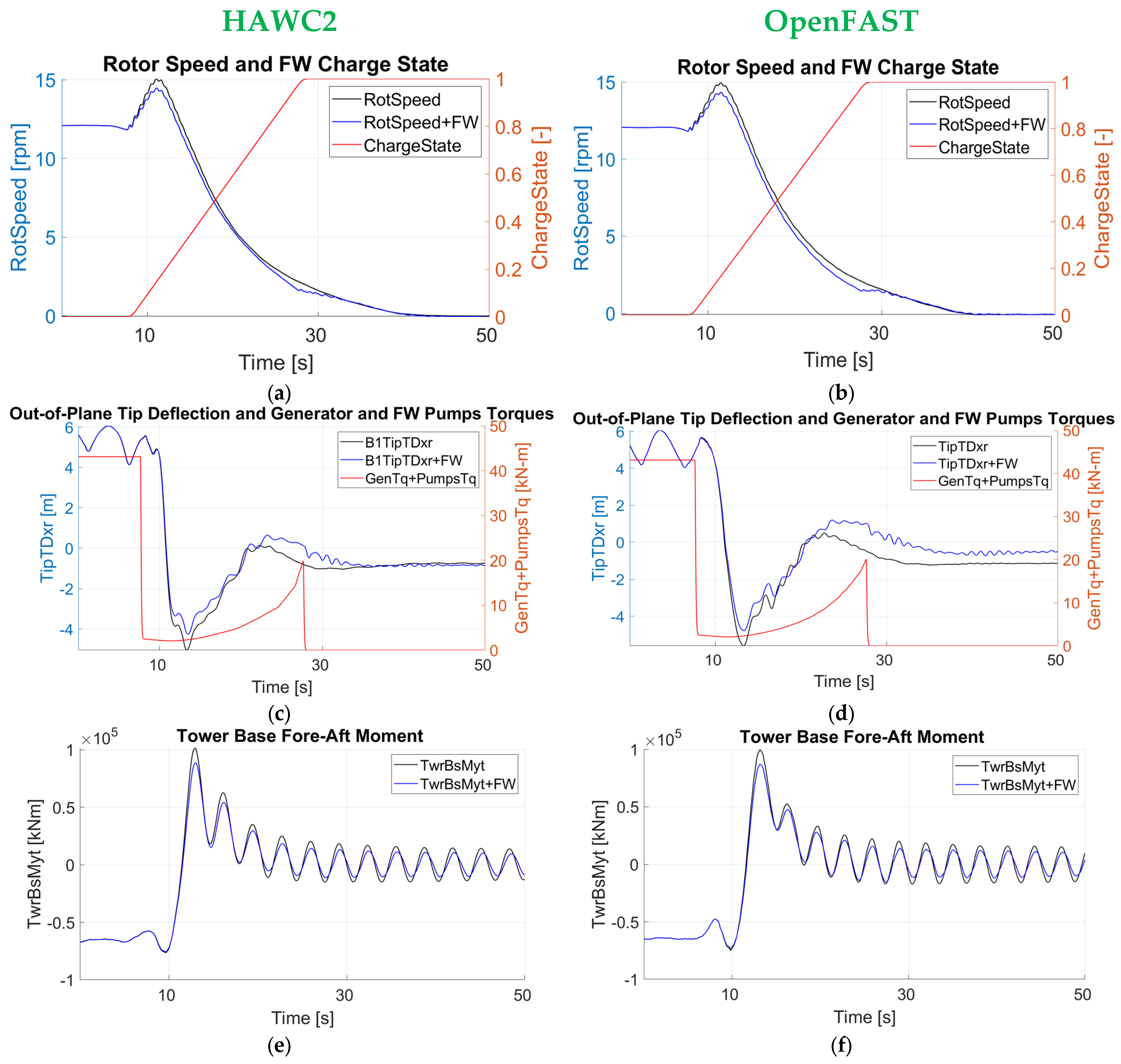
Since the aerodynamics models of HAWC2 and OpenFAST are not in the scope of the study presented in this paper, the difference in these aerodynamics models is not further investigated. However, to evaluate the effect of the flywheel on the 5 MW wind turbine without the effect of the difference in the aerodynamics models, two comparisons are presented in Figure 12: 5 MW wind turbine with and without flywheel in OpenFAST (Figure 12 right-hand side), and 5 MW wind turbine with and without flywheel in HAWC2 (Figure 12 left-hand side).

As the generator torque disappears due to the sudden grid loss, see Figure 11a, the wind turbine has to be brought to a standstill fast to avoid excessive overspeed. This is done by quickly pitching the blade to a feather position from 0° to 90°, see Figure 11b, i.e., aerodynamic emergency braking. However, the quick pitching at high rotor speeds leads to an increase in the mechanical loads on the wind turbine support structures. This can be seen in Figure 11d as an increase in the tower base fore-aft moment.

The flywheel can support the aerodynamic emergency breaking in the case of DLC 2.3 by charging the flywheel to reach its maximum charge state in all three blades, see Figure 12a,b. Charging the flywheel produces two decelerating torques: a mechanical decelerating torque resulting from the Coriolis forces, see Section 2.2.2, and an electrical decelerating torque at the generator by the electric pumps, see Figure 12c,d. The pumps support the charging process of the flywheel and draw their power from the wind turbine generator, even when the wind turbine is no longer connected to the grid. In this state of operation, the generator with its frequency converter and the motors of the pumps is an electric island. Figure 12c,d illustrates the damping effect of the flywheel mechanical decelerating torque on the out-of-plane blade tip deflection. Figure 12a,b shows that the rotor speed accelerates less when the flywheel is applied. The flywheel can decrease the tower base fore-aft moment by up to 12.5%, see Figure 12e,f.

5. Conclusions

Previous studies have investigated the effect of variable blade inertia on wind turbines using the First Eigenmodes simulation model [15] and the modified code of ElastoDyn [18]. The restrictions of these models and the simplified assumptions about the method used to implement variable blade inertia have necessitated an improvement to this method in more advanced structural dynamics models of wind turbine rotor blades. This paper presents a comparison, validation, and application of two improved methods to enable the structural dynamics models of HAWC2 and BeamDyn to simulate wind turbines with variable blade inertia. These two advanced models were developed to represent the nonlinear structural behavior of modern wind turbine composite blades. Hence, they are the ideal choice for representing the extended functionality of variable blade inertia presented in this paper.

This paper focuses on the variation of the blade inertia from the application of flywheels in wind turbine rotors. Two methods were developed to be implemented in HAWC2 and BeamDyn. These methods were validated based on three benchmarking cases of increasing complexity. The validation showed very good agreement between BeamDyn, HAWC2, and analytical calculations for all three cases.

Simulating the application of the flywheel in the rotor blades of the NREL 5 MW reference wind turbine when it is subject to DLC 2.3 shows that the flywheel reduces the tower base fore-aft bending moment by 12%. This result can be yielded with both HAWC2 and OpenFAST. With the variable blade inertia, the simulated effect of the flywheel shows good agreement between HAWC2 and OpenFAST in the rotor blade motions, e.g., the rotor speed and the out-of-plane motion, as well as in the tower base torque.

The focus of the current research project is on the enhancement of HAWC2 and BeamDyn to simulate wind turbines with hydraulic-pneumatic flywheels. Since this paper shows that this goal is achieved, future work will focus on the applications of these tools to simulate different wind turbine types with flywheels.