Energy Management of Microgrids with a Smart Charging Strategy for Electric Vehicles Using an Improved RUN Optimizer

Abstract

Electric vehicles (EVs) and renewable energy resources (RERs) are widely integrated into electrical systems to reduce dependency on fossil fuels and emissions. The energy management of microgrids (MGs) is a challenging task due to uncertainty about EVs and RERs. In this regard, an improved version of the RUNge Kutta optimizer (RUN) was developed to solve the energy management of MGs and assign the optimal charging powers of the EVs for reducing the operating cost. The improved RUN optimizer is based on two improved strategies: Weibull flight distribution (WFD) and a fitness–distance balance selection (FDB) strategy, which are applied to the conventional RUN optimizer to improve its performance and searching ability. In this paper, the energy management of MGs is solved both at a deterministic level (i.e., without considering the uncertainties of the system) and while considering the uncertainties of the system, with and without a smart charging strategy for EVs. The studied MG consists of two diesel generators, two wind turbines (WTs), three fuel cells (FCs), an electrical vehicle charging station and interconnected loads. The obtained results reveal that the proposed algorithm is efficient for solving the EM of the MG compared to the other algorithms. In addition, the operating cost is reduced with the optimal charging strategy.

1. Introduction

A microgrid (MG) can be defined as interconnected loads with distrusted generators (DGs) and energy storage systems that are connected to the grid (on-grid MG) or work autonomously (isolated MG) [1]. The MGs can provide the required energy for different customers, including commercial, residential and industrial loads [2]. Several benefits are obtained from MG implementation, including improvements in system reliability, reduced operating costs, resolution of system losses and overload problems, energy supply decentralization and emission reductions [3].

Use of electric vehicles (EVs) and renewable energy-based DGs (RDGs) like solar PV, wind turbines (WTs), hydropower and biomass has greatly increased for many reasons, including reduced dependence on conventional fuel-based DGs, reduced greenhouse gas emissions and the sustainability of electrical systems. The main feature of RDGs and EVs is their stochastic nature and uncertain behavior. Thus, solving the energy management (EM) of the MGs with EVs and RDGs is a challenging task. A scenario-based method was applied for solving the EM of MGs considering the uncertain parameters of RDGs and the loading [4]. The EM was solved using the equilibrium optimizer (EO) for multi-objective functions in the presence of WTs and PVs and with uncertainty of these resources and the load demand [5]. In [6], the EM problem was solved by considering the demand response and the uncertainties of the RDGs. A microgrid central controller was utilized for the EM of the MG and consists of PV-, WT- and biomass-based generators [7]. In [8], the EM of the MG was solved using mixed-integer programing with demand-side management in the presence of portable RDGs. Integrated multidimensional modeling software was implemented for the EM solution of MGs and consisted of RDGs, FCs and a combined heat and power unit [9]. The EM of an MG that consisted of WT, FCs, PV, batteries and diesel generators was solved using the genetic algorithm [10]. An $\mathsf{\epsilon }$-constraint approach was employed for solving the energy management of the MG [11] in the presence of a tidal turbine, PV and WT [11]. Although these studies solved the EM of the RDGs, the integration of EVs was not considered.

Several attempts have been made to solve the EM of EVs where mixed-integer quadratic programming was implemented considering charging and discharging of the EVs [12]. The EM was solved for an AC/DC microgrid in the presence of RDGs considering charging and discharging of the EVs using information gap decision theory [13]. Hong’s 2m point estimate method was applied to solve the EM of an MG considering the different charging mechanisms [14]. It is worth mentioning here that the previous study did not take everything into account (e.g., fuel cells). ε-constraint and decision maker were implemented for the EM solution of a residential MG with EVs, RDGs and batteries [15]. Although the EM solved uncertainties of the system, the smart charging of EVs was not discussed.

The RUN optimizer is a novel optimizer that mimics solving the differential equations. The optimizer is used for solving several problems like optimal ratings of microgrid components [16], hydropower plant operation [17], PV parameters [18], photovoltaic modeling [19], energy management with demand-side response [20], fractional-order design of batteries [21], optimal PID of an AVR system [22], cancer classification [23] and the equations of energy balance for an inverted absorber [24].

Selection strategy methods have been widely implemented in the meta-heuristic optimization algorithm for improving their global searching ability as well as the diversity of these techniques. The selection strategy can be divided into three categories: deterministic, non-deterministic and probabilistic. In the non-deterministic method, solution candidates are selected randomly from the population [25,26]. Fitness–distance balance (FDB) is a common selection method that has been applied for improving the performance of optimization algorithms [27] like the stochastic fractal search algorithm [28], differential evolution [29], moth swarm algorithm [30], particle swarm optimizer [31], wind-driven optimization [32] and coyote optimization [33]. Improving the searching ability of the RUN technique using FDB was presented in [34,35].

In this work, the EM of an MG is solved in the presence of EVs while considering different uncertain parameters using an improved version of the RUN optimizer based on FDB and Weibull flight distribution. The conventional RUN and improved RUN techniques are with and without uncertainties. The studied MG consists of two diesel generators, two wind turbines (WTs), three fuel cells (FCs), an electrical vehicle charging station and interconnected loads. The rest of this work is laid out as follows. Section 2 describes the objective function that is associated with MG energy management and representation of the DGs. Section 3 explains the concept and steps of the RUN optimizer, while Section 4 presents an overview of the improved RUN technique. Section 5 shows the models of the uncertainties. Section 6 contains the numerical results and corresponding discussion. Section 7 concludes the findings and results and the main concepts. The novelty and contributions of the paper are depicted in the revised paper.

The novelty and contributions of the paper can be outlined as follows:

• The stochastic energy management of an MG is solved with implementation of a smart charging strategy for EVs.
• An improved version of the RUN optimizer based on FDB and Weibull flight distribution is proposed for solving the energy management problem.
• Energy management of the MG is solved at a deterministic level for cost reduction using the proposed optimizer; the obtained results are compared to other optimization algorithms.
• Energy management of the MG is solved by considering the uncertainties of the EVs, load and output power of the WTs.

2. Problem Formulation

2.1. Objective Function

The aim of this work is to reduce the operating cost of the smart grid in the presence of two diesel generators, three fuel cells, two wind turbines and an electrical vehicle charging station. The considered objective function is represented as follows [36]:

$$C_{total}=C_D+C_{WT}+C_{FC}$$

(1)

where $C_D$, $C_{Wind}$ and $C_{FC}$ are the operation costs of the diesels, WTs and FCs, respectively. The cost of the WT can be calculated as follows:

$$C_{WT}=\sum _{n=1}^{NWT}\left(K_n{P}_{WT,n}\right)$$

(2)

in which

$$P_{WT}\left(w\right)\hspace{0.33em}\hspace{0.33em}=\left\{\hspace{0.33em}\begin{array}{ccc}0& for& w<w_i and w>w_o\\ P_r\left(\frac{w-w_i}{w_r-w_i}\right)& for& \left(w_i\le w\le w_r\right)\\ P_r& for & \left(w_r<w\le w_o\right)\end{array}\right.$$

(3)

where $K_n$ is the operation and maintenance cost of the WT. $P_{WT}$ is the power generated by the WT while $P_r$ is its rated power. $w_o$, $w_r$, and $w_i$ are the cut-out, the rated, and the cut-in wind speeds, respectively. NWT refers to the number of wind turbines. The operation cost of the diesel DG generator is represented as follows [37]:

$$C_{Diesel}=\sum _{i=1}^{NDG}{a}_i{P}_{i,t }^2+b_i{P}_{i,t}+c_i$$

(4)

where, $a_i,b_i$ and $c_i$ denote the coefficients of the cost of the ith generator. NDG refers to the number of diesel generators in the MGs. The third term in Equation (1) represents the operation cost of the FC, which is calculated as follows [38]:

$$C_{FC}={\omega }_n \sum _{k=1}^{NFC}\frac{P_{FC,k}}{{\eta }_{FC,k}}$$

(5)

where, $NFC$ represents the number of FCs in the MG. $P_{FC}$ represents the output power from FCs. ${\omega }_n$ and ${\eta }_{FC}$ denote the cost of the natural gas and the efficiency of the FC. The mathematical model of the EV is related to its battery, including its state of charge ($SOC$), the charging power ($P_{CH}$), the discharging power ($P_{DC}$) and the efficiencies of the charging (${\eta }_{CH}$) and the discharging (${\eta }_{DC}$). The state of charging is represented as follows:

$$SO{C}_i^t=SO{C}_i^{t-1}+{\eta }_{CH,i}{P}_{CH,i}^t\mathsf{\Delta }t\delta -\frac{\mathsf{\Delta }t\gamma P_{DC,i}^t}{{\eta }_{DC,i}}$$

(6)

2.2. Constraints

(a)

Equality Constraints

These constraints refer to the balanced power in the electric system, which can be described as follows:

$$P_{WT}+P_{FC}+P_i=P_{load}+P_{CH}-P_{DC}$$

(7)

(b)

Inequality Constraints

These constraints refer to the allowable limits of the variables of the system, which are described as follows:

$$P_i^{min}\le P_i\le P_{i }^{max}$$

(8)

$$P_{FC}^{min}\le P_{FC}\le P_{FC }^{max}$$

(9)

$$P_r^{min}\le P_r\le P_{r }^{max}$$

(10)

$${SOC}^{min}\le SOC\le {SOC}^{max}$$

(11)

$$P_{CH }^{min}\le P_{CH}\le P_{CH }^{max}$$

(12)

where $min$ and $max$ superscripts refer to the minimum and the maximum limits.

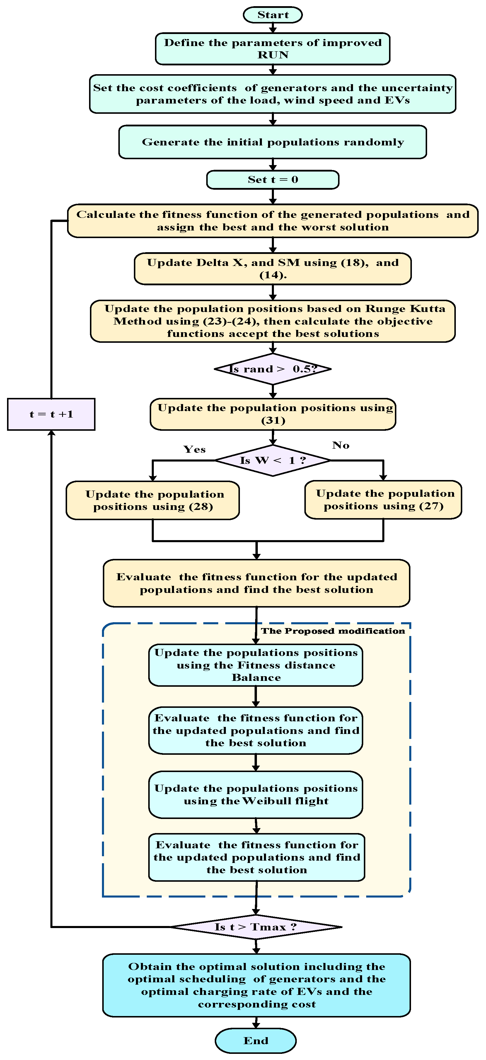
3. RUNge Kutta Optimizer (RUN)

RUN is a new optimization technique that simulates the Runge Kutta method (RKM) for the differential equation’s solution. The RUN technique is based on two strategies—the first strategy is based on the Runge Kutta method, while the second strategy is based on the enhanced solution quality strategy (ESQ) [39,40]. The step procedure of the RUN algorithm can be summarized as follows:

• Step 1: Initialization

The initial populations will be generated randomly using (13) as follows:

$$X_j^i={Lower}_j+\left({Upper}_j-{Lower}_j\right)\times rand$$

(13)

where $Lower$ and $Upper$ represent the lower and upper boundaries of variables.

• Step 2: Root of the search mechanism

This step simulates the RKM, which can be described as follows:

$$SM=\frac{1}{6}\left(x_{RK}\right)\mathsf{\Delta }x$$

(14)

in which

$$x_{RK}=k_1+2\times k_2+2\times k_3+k_4$$

(15)

where $k_1$, $k_2$, $k_3$ and $k_4$ refer to the weighted values, which can be formulated as follows:

$$k_1=\frac{1}{2\mathsf{\Delta }x} \left(rand\times x_w-u\times x_b\right)$$

(16)

$$u=\mathit{round}(1+rand)\times (1-\mathit{rand})$$

(17)

where $\mathit{rand}$ refers to a random number in range [0–1], $u$ refers to a random value that is used to increase the importance of the best location, and $x_w$ and $x_b$ are the worst and the best solutions, respectively. $\mathsf{\Delta }x$ is depicted as follows:

$$\mathsf{\Delta }x=2\times rand\times \left(rand\times \left(\left(x_b-\right.\right.rand\left.\left.\times x_{avg}\right)+\gamma \right)\right)$$

(18)

$$\gamma =rand\times \left(x_n-rand\times (u-l)\right)\times exp\left(-4\times \frac{i}{\mathit{Maxi}}\right)$$

(19)

$$k_2=f\left(x+\frac{\mathsf{\Delta }x}{2},y+\frac{\mathsf{\Delta }x}{2}\times k_1\right)$$

(20)

$$k_3=f\left(x+\frac{\mathsf{\Delta }x}{2},y+\frac{\mathsf{\Delta }x}{2}\times k_2\right)$$

(21)

$$k_4=f\left(x+\mathsf{\Delta }x,y+\mathsf{\Delta }x\times k_3\right)$$

(22)

• Step 3: Updating the solution

In this step the populations will update their locations based on a unique exploitation and exploration mechanism according to the following equations:

$${ x}_{n+1}=\left(x_c+r\times SF\times g\times x_c\right)+SF\times SM+\mu \times x_s \mathit{rand} <0.5$$

(23)

$$x_{n+1}=\left(x_m+r\times SF\times g\times x_m\right)+SF\times SM+\mu \times x_s \mathit{rand} \ge 0.5$$

(24)

in which

$$SF=2·(0.5-rand)\times f$$

(25)

$$f=a\times exp\left(-b\times \mathit{rand}\times \left(\frac{i}{T_{max}}\right)\right)$$

(26)

where $r$ represents an integer number equals to 1 or −1, $g$ represents a random value in the range [0, 2] and $a$ and $b$ refer to constant values. $T_{max}$ denotes the maximum iteration number.

• Step 4: EQS updating

The EQS method depends upon updating the locations of the populations using the average of three populations and the best solution. The EQS can be described as follows:

If $rand<0.5$

If $w<1$

$$x_{new2}=x_{new1}+r\cdot w\cdot \left|\left(x_{new1}-x_{avg}\right)+randn\right|$$

(27)

then

$$x_{new2}=\left(x_{new1}-x_{avg}\right)+r\cdot w\cdot \mid \left(u\cdot x_{new1}-x_{avg}\right)+randn\mid$$

(28)

End

End

$$w=rand(\mathrm{0,2})\cdot exp\left(-c\left(\frac{i}{T_{max}}\right)\right)$$

(29)

$$x_{avg}=\frac{x_{r1}+x_{r2}+x_{r3}}{3}$$

(30)

$$x_{new1}=\beta \times x_{avg}+(1-\beta )\times x_{\mathit{best} }$$

(31)

where $0\le \beta \le 1$. $c=5\times rand$. $w$ is a random factor that decreases with iteration. If the new solution is worse than the current solution, it will be updated as follows:

$$x_{\mathit{new}3}=\left(x_{\mathit{new}2}-\mathit{rand}{x}_{\mathit{new}2}\right)+SF\times \left(\mathit{rand}{·x}_{RK}+\left(v·x_b-x_{\mathit{new}2}\right)\right) \mathrm{if} \mathit{rand}<w$$

(32)

where $v=2\times rand$. To depict the procedure of the EQS, Algorithm 1 lists the pseudocode of the EQS.

Algorithm 1. The pseudocode of the EQS

Update the value of $w$ using (29). Find the $x_{new1}$ using (31).   if  $rand<0.5$  if  $w<1$    Update $x_{new2}$ using (27). else    Update $x_{new2}$ using (28). end end   if  $f\left(x_n\right)<x_{new2}$   if  $rand<w$    Update $x_{new3 }$ using (32).   end end

4. The improved RUNge Kutta Optimizer (IRUN)

To overcome the stagnation of the conventional RUN optimization technique, the balance selection method is utilized to improve the exploitation phase of the proposed algorithm, while the Weibull Flight is proposed for improving its exploration phase.

4.1. Weibull Flight Distribution

Generally the cumulative Weibull distribution is based on two factors, the shape ($v$) and the scale factor ($u$), that can be described as follows [41]:

$$f(x)=\frac{v}{u}{\left(\frac{x}{u}\right)}^{v-1}{e}^{-{\left(\frac{x}{u}\right)}^v};x\ge 0$$

(33)

Two movements can be obtained from the Weibull distribution, including the wide step movement and small step movement. The wide step movement can be given as follows:

$$\mathit{Step}= \mathit{wblrnd} (\mathrm{1,1},[1,D\left]\right)\times sign\left(rand\right(1,D)-0.5)$$

(34)

wblrnd is a random number that is generated from the Weibull distribution. sign() provides values −1, 0 and 1. The small step movement can be given as follows:

$$Step=\left\{\begin{array}{l}wblrnd(\mathrm{0.5,1},[1,D\left]\right)\cdot \times 0.5\ast sign\left(rand\right(1,D)-0.5)\\ \times norm\left(x_{\mathit{best} }-x_i\right),if{x}_{\mathit{best} }\ne x_i\\ wblrnd(\mathrm{0.5,1},[1,D\left]\right)\cdot \times 0.1\times sign\left(rand\right(1,D)-0.5),else\end{array}\right.$$

(35)

The new generated location of the population can be calculated as follows:

$$x_{\mathit{new},\mathrm{i}}=x_{\mathit{new},\mathrm{i}}+Step$$

(36)

4.2. The Fitness–Distance Balance (FDB)

The FDB method is one of the most robust selection methods that has been implemented for enhancing the performance of optimization techniques [27]. FDB is based on the distance between the selected candidates and the best solution as well as the fitness function values of the candidates. A distance vector and fitness function vector are constructed as follows:

$$DX\equiv {\left. [\begin{array}{c}{DX}_1\\ ⋮\\ {DX}_m\end{array}\right]}_{mx1}$$

(37)

$$F\equiv {\left. [\begin{array}{c}{f}_1\\ ⋮\\ f_m\end{array}\right]}_{mx1}$$

(38)

in which

$$D_{X_i}=\sqrt{{\left.{\left(x_{1\left[i\right]}-x_{1\left[\mathit{best}\right]}\right)}^2+\left(x_{2\left]i\right]}-x_{2]best}\right]\right)}^2+\cdots \&+{\left(x_{n\left[i\right]}-x_{n\left[\mathit{best}\right]}\right)}^2}$$

(39)

The scores of the populations are calculated based on the normalized fitness functions ($norm{F}_i$) and the normalized distances ($norm{D}_{X_i}$) as follows:

$$S_{P_i}=w\times norm{F}_i+(1-w)\times norm{D}_{X_i}$$

(40)

where $w$ is a weight factor between 0 and 1. Figure 1 shows application of the suggested improved RUN technique for the solution of the energy management.

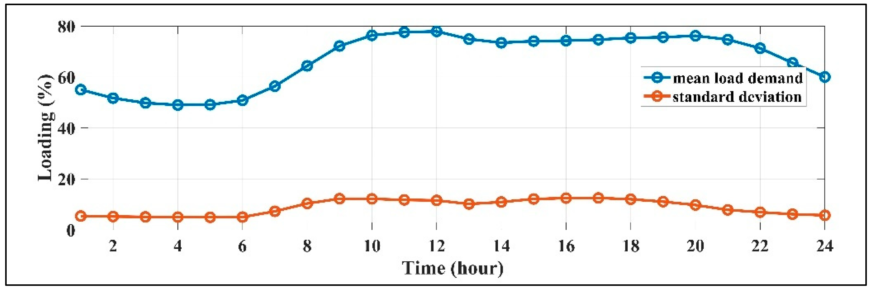
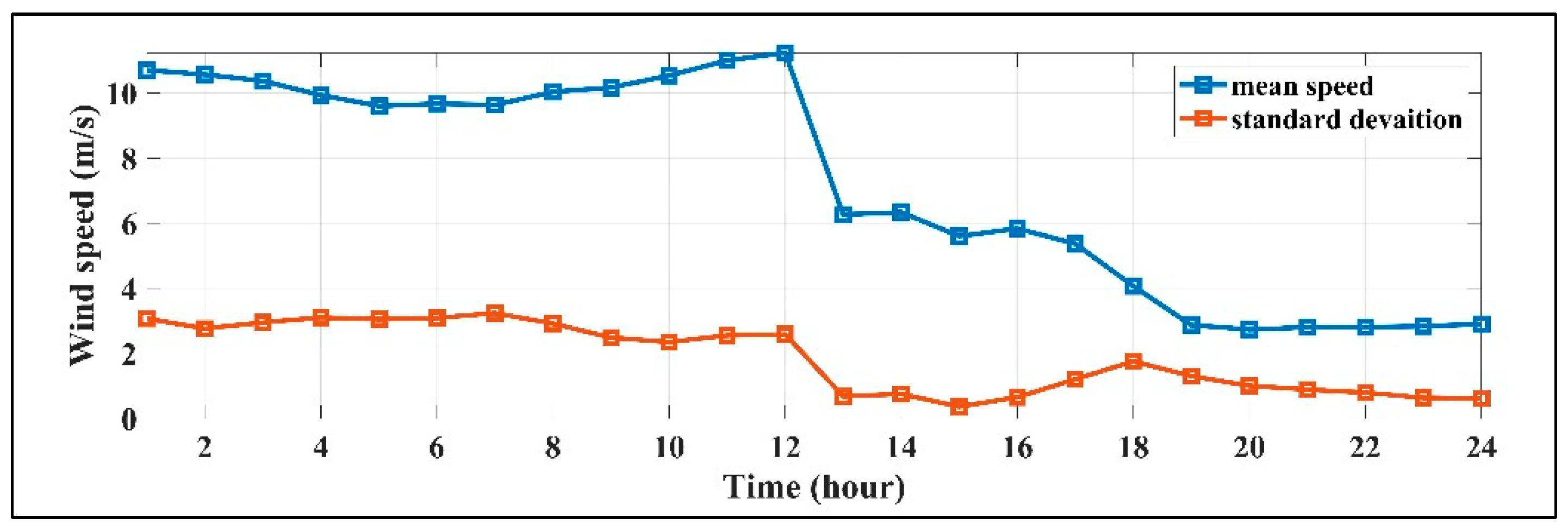
5. Uncertainty Representation

In this work two uncertain parameters have been taken into consideration, including the load demand, which can be modeled using the normal PDF, while the wind speed can be modeled using the Weibull PDF. The normal PDF of the load demand is formulated using (41) [42].

$$f_L(S_L)=\frac{1}{\sqrt{2\pi {\sigma }_L}}exp\left. [-\frac{(S_L-{\mu }_L)2}{2{{\sigma }_L}^2}\right]$$

(41)

where ${\sigma }_L$ and ${\mu }_L$ refer to the standard deviation and the mean value of loading. The Weibull PDF of the wind speed is formulated using (42) [43,44].

$$f(w)=\left(\frac{k}{c}\right){\left(\frac{w}{c}\right)}^{k-1}exp\left. [-{\left(\frac{w}{c}\right)}^k\right]$$

(42)

where $c$ represents the scale parameter of the wind speed, while $k$ is the shape parameter. The shape and the scale parameters are obtained from the mean (${\mu }_w$) and the standard deviation (${\sigma }_w$) as follows [45]:

$$k^t={\left(\frac{{\sigma }^t}{{\mu }_w^t}\right)}^{-1.086}$$

(43)

$$c^t=\frac{{\mu }_w^t}{\Gamma \left(1+1/k^t\right)}$$

(44)

Figure 2 and Figure 3 show the mean and the standard deviation of the loading and the wind speed, respectively. Then, the Monte Carlo simulation method (MCS) [46] is implemented for generating a set of scenarios for each hour of the load and the wind speed. Here, 1000 scenarios were obtained from the MSC method for each hour. Then the scenario-based method [47,48] was utilized for reducing the huge number of scenarios to 25 scenarios.

Two stochastic parameters are associated with the electric vehicles, including the arrival time and the state of charge that are modeled using the normal PDFs as follows [49]:

$$f_n^t\left(T_A\right)=\frac{1}{{\sigma }_{TA}\sqrt{2\pi }}\times exp\left. [-\left(\frac{{\left(T_A-{\mu }_{TA}\right)}^2}{2{\left({\sigma }_{TA}\right)}^2}\right)\right]$$

(45)

$$f_n^t(SOC)=\frac{1}{{\sigma }_{SOC}\sqrt{2\pi }}\times exp\left. [-\left(\frac{{\left(SOC-{\mu }_{SOC}\right)}^2}{2{\left({\sigma }_{SOC}\right)}^2}\right)\right]$$

(46)

${\sigma }_{TA}$ and ${\mu }_{TA}$ are the standard deviation and the mean values of the arrival time of the EV, respectively. ${\sigma }_{TA}$ and ${\mu }_{TA}$ are the standard deviation and the mean values of the state of charge.

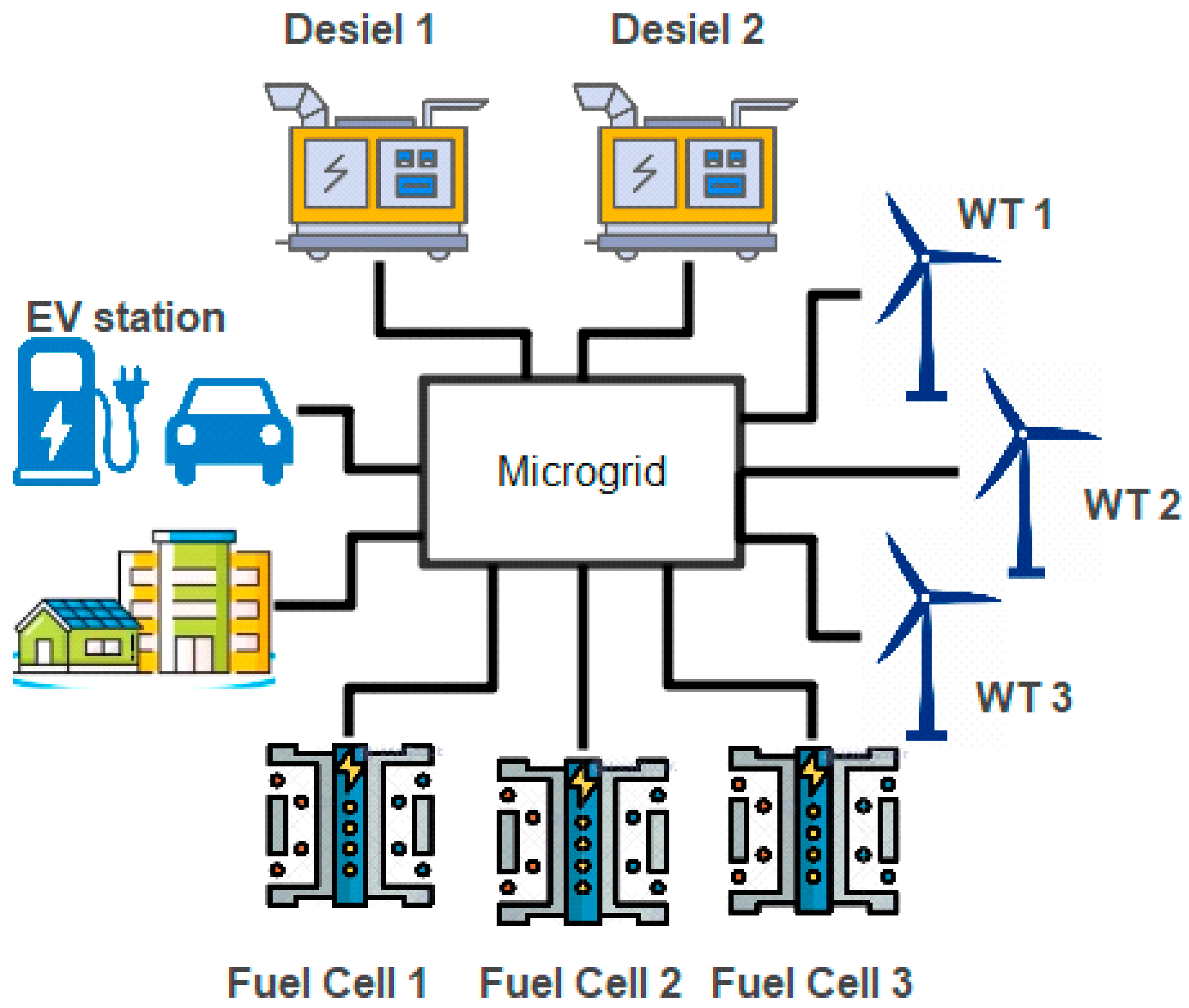
6. Simulation Results

In this section the energy management of the MG is solved using the conventional RUN and the improved RUN techniques with and without uncertainties. The studied MG consists of two diesel generators, two wind turbines (WTs), three fuel cells (FCs), an electric vehicle charging station and interconnect loads as illustrated in Figure 4. The cost coefficients of the diesel generators, FCs and WTs are listed in

Table 1. The generator data of the studied MG.

Generation Type	a (USD/(kWh)2)	b (USD/kWh)	c (USD/h)	${\mathit{P}}_{}^{\mathit{m}\mathit{i}\mathit{n}}$ (kW)	${\mathit{P}}_{}^{\mathit{m}\mathit{a}\mathit{x}}$ (kW)	${\mathit{V}}_{\mathit{i}}$ $(\mathbf{m}/\mathbf{s})$	${\mathit{V}}_{\mathit{o}}$ $(\mathbf{m}/\mathbf{s})$	${\mathit{V}}_{\mathit{r}}$ $(\mathbf{m}/\mathbf{s})$	${\mathsf{\eta }}_{\mathbf{F}\mathbf{C}}$ (%)
Diesel 1	0.0074	0.2333	0.4333	0	400	-	-	-	-
Diesel 2	0.0042	0.1453	0.2731	0	800	-	-	-	-
FC 1	0	0.05	0	0	150	-			90
FC 2	0	0.05	0	0	100	-	-	-	90
FC 3	0	0.07	0	0	100	-	-	-	85
WT1	0	0.022	0	0	300	5	15	10	-
WT2	0	0.032	0	0	300	5	15	10	-

. The simulation results were conducted using MATLAB software (MATLAB R2021a) on a Core I7 PC with 2.90 GHz and 32 GB RAM. The selected numbers of populations and iterations of the RUN and the improved RUN techniques are 50 and 200, respectively. The studied cases are presented as follows:

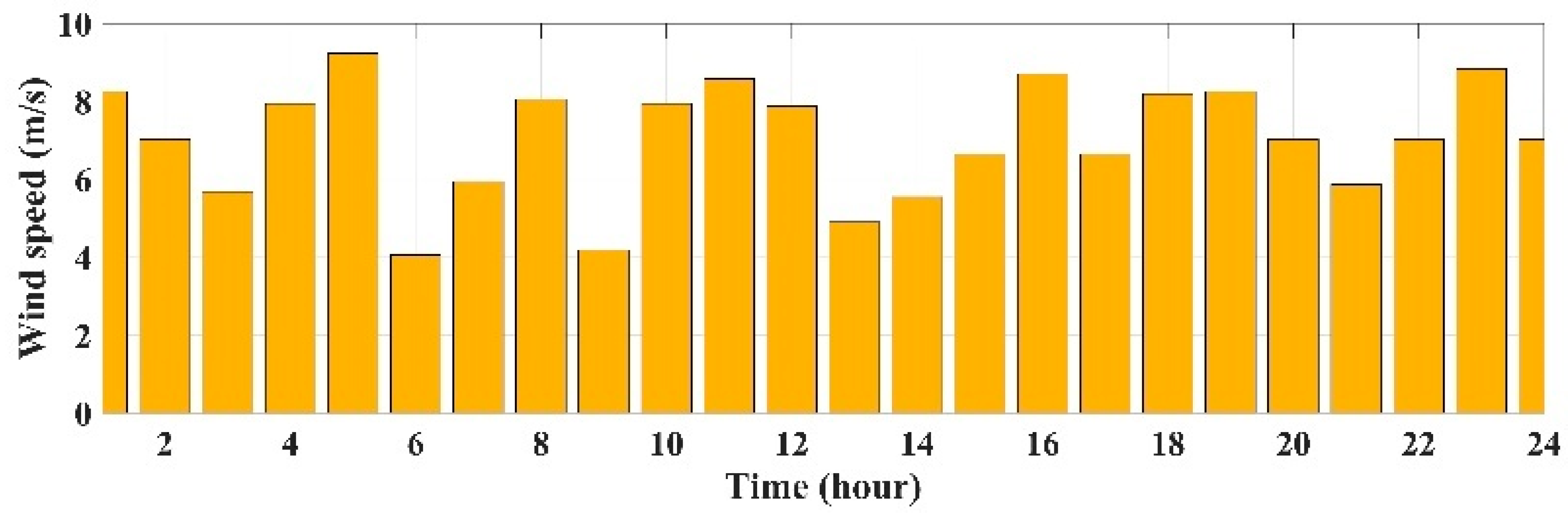
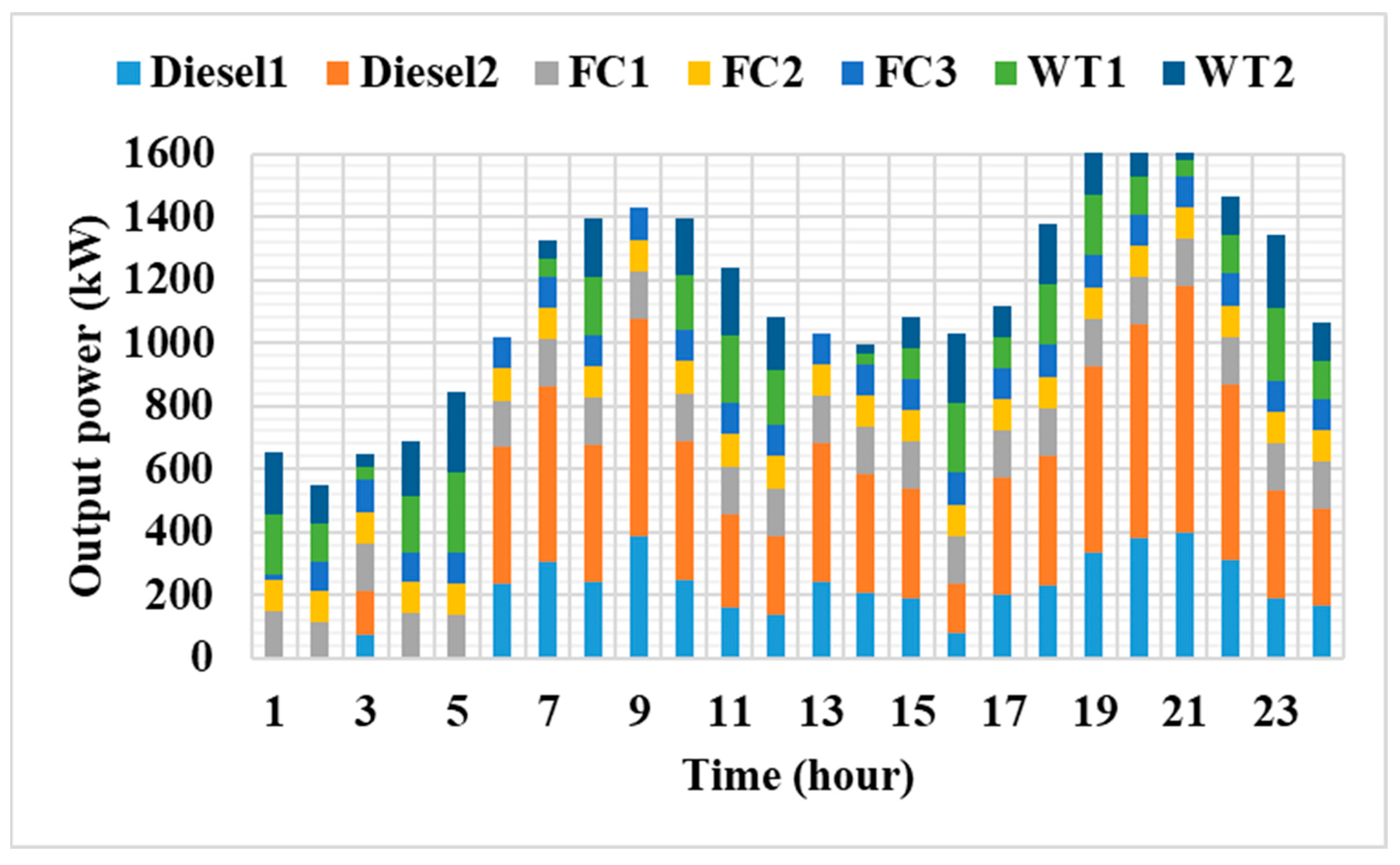
6.1. Case 1: Solving the Energy Management in a Deterministic Condition

In this section, the RUN and the suggested improved RUN are applied for solving the energy management of the MG without considering the uncertainty of the system for verifying the effectiveness of the proposed optimization algorithm. The load profile of the system is depicted in Figure 5, while the wind speed is illustrated in Figure 6. The obtained minimum operation costs via 25 runs by RUN and the improved RUN were USD 29,893.7746 and USD 30,779.9573, respectively.

Table 2. Statistical comparison of the day-ahead scheduling by applying different optimization techniques for Case 1.

Algorithm	Improved RUN	RUN	EO [38]	CSA [37]	DE [37]	MOSHEPO [50]
Cost (USD)	29,893.7746	30,779.9573	33,100	33,824.10	33,930.94	33,804.53
The reduction of cost v.s. Improved RUN	-	2.879%	9.687%	11.619%	11.898%	11.569%

lists the operating costs that were obtained using other techniques. From Table 2, the reductions in the cost compared to the improved RUN using the conventional RUN, the Equilibrium Optimizer (EO) [38], the cuckoo search algorithm (CSA) [37], the differential evolution (DE) [37] and the spotted hyena and emperor penguin optimizer (MOSHEPO) [50] are 2.879%, 9.687%, 11.619%, 11.898% and 11.569%, respectively.

The optimal scheduling for this case obtained using the RUN and the improved RUN are depicted in Figure 7 and Figure 8, respectively. According to Figure 7 and Figure 8, the output powers of WT1 and WT2 are varied with the wind speed variations. In addition, providing the required powers from the WTs to maximum utilization of the renewable energy resource were prioritized. The FCs were the second-priority resources. This was due to their inferior fuel costs compared to the diesel generators. The convergence curves of the RUN and the improved RUN optimization algorithms for the cost reduction are shown in Figure 9. It is evident that the proposed algorithm has stable characteristics compared to the conventional RUN, where the suggested algorithm was converged at the 146th iteration.

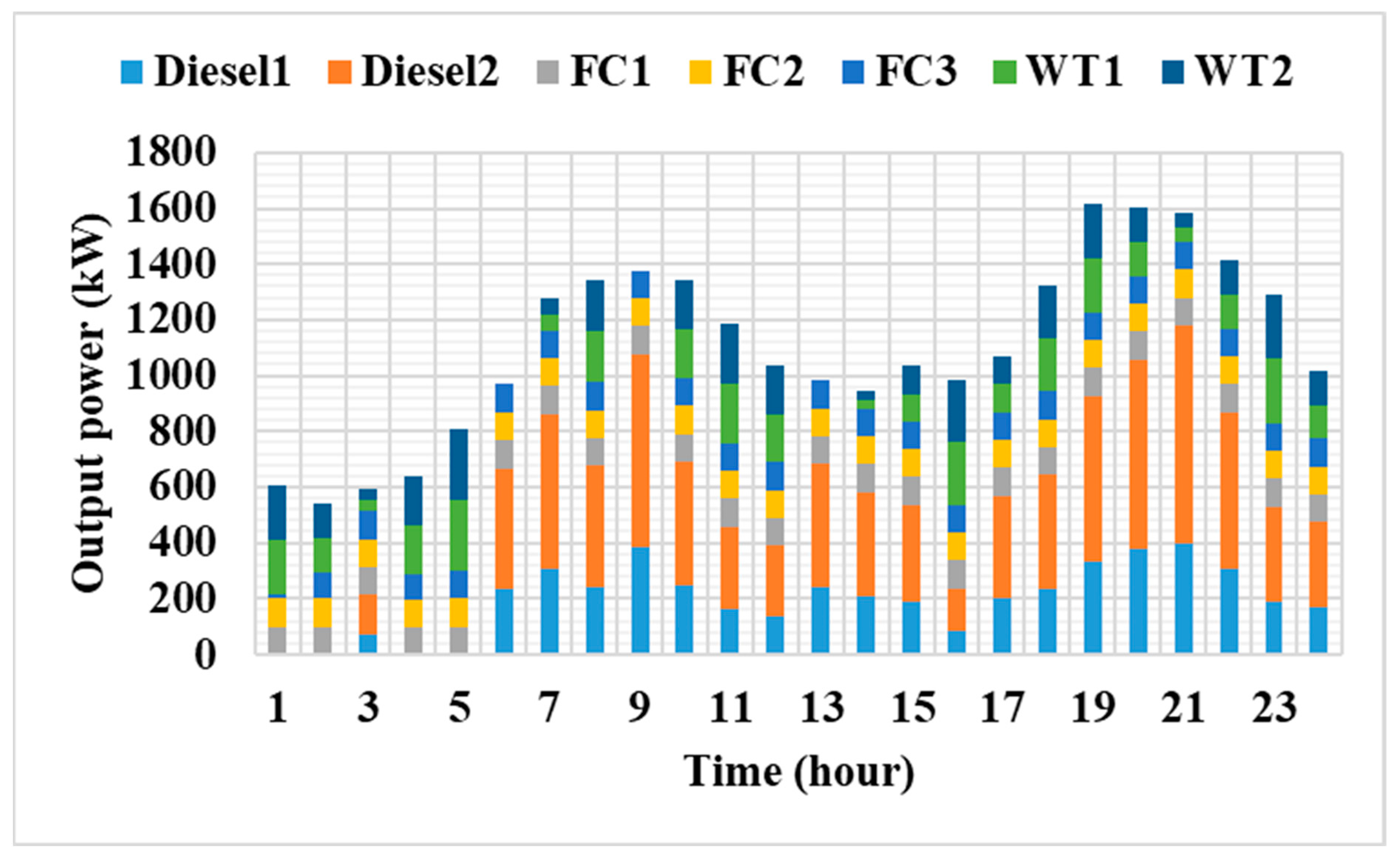
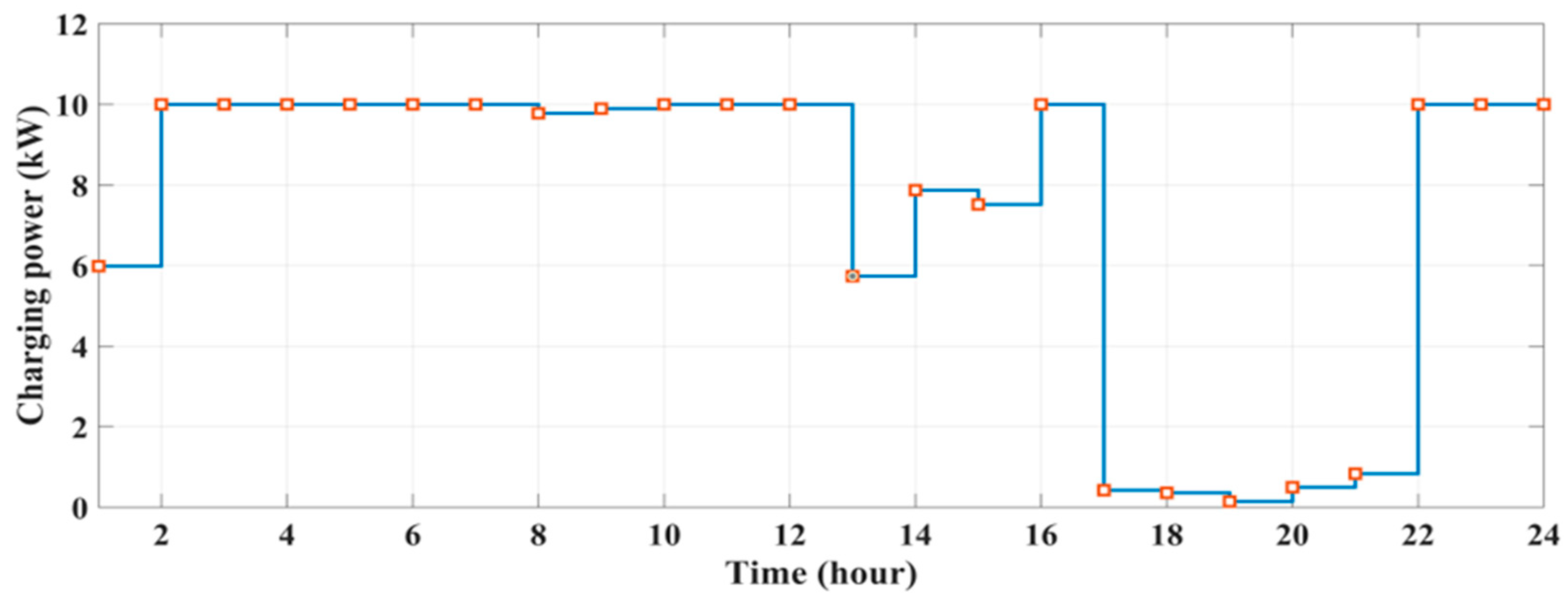
6.2. Case 2: Solving the Energy Management with EVs in a Stochastic Condition

In this section, the proposed algorithm was employed for EM solution with inclusion of the EVs’ charging station with and without considering the smart charging strategy of the EV. The EM was solved by considering the uncertainties of the load demand, the wind speed, the state of charge and the arrival time of the EVs. The capacity of the battery found in the EVs was 50 kWh, while its maximum charging rate was 10 kW [51]. The minimum allowable limit of the EVs’ SOC was 15% of the battery’s capacity, and the EV left the station when its charging capacity was at least more than 90%. The mean (${\mu }_{SOC}$) and the standard deviation of the (${\sigma }_{SOC}$) of the initial state of charge were selected to be 50% and 14%, respectively [49]. The mean (${\mu }_{TA}$) and the standard deviation (${\sigma }_{TA}$) of the arrival time were selected to be 18 and 5, respectively [52]. The expected load demand and the wind speed are depicted in Figure 10 and Figure 11, respectively. The charging station consists of 100 EVs, and the states of the charge of each EV are depicted in Figure 12. The energy management of the EVs is solved with and without considering the smart charging strategy of the EVs. With the conventional charging strategy, the EVs charged with a maximum charging rate, i.e., 10 kW, while in the smart charging strategy, the EVs charged with optimal controlling of the charging rate.

Table 3. The simulation results with conventional charging strategy.

Time	Diesel 1	Diesel 2	FC 1	FC 2	FC 3	WT 1	WT 2	Load	EV Loading
1	0.00	0.06	133.94	98.76	95.78	300.00	300.00	918.54	10.00
2	0.07	0.00	149.99	42.21	100.00	300.00	300.00	862.27	30.00
3	0.10	0.00	95.68	100.00	100.00	300.00	300.00	829.84	65.94
4	0.06	1.22	150.00	99.99	100.00	283.54	283.54	813.42	104.93
5	37.58	78.14	150.00	100.00	100.00	264.36	264.36	825.26	169.17
6	42.97	88.98	150.00	100.00	100.00	288.67	288.67	836.88	222.41
7	137.52	254.20	150.00	100.00	100.00	261.36	261.36	964.94	299.50
8	213.75	383.18	150.00	100.00	100.00	262.55	262.55	1110.03	362.00
9	217.92	392.53	150.00	100.00	100.00	300.00	300.00	1213.37	347.08
10	196.16	360.11	150.00	100.00	100.00	300.00	300.00	1296.35	209.93
11	202.09	365.88	150.00	100.00	100.00	300.00	300.00	1286.07	231.90
12	219.02	394.62	150.00	100.00	100.00	300.00	300.00	1307.51	256.13
13	354.81	634.77	150.00	100.00	100.00	70.41	70.41	1250.52	229.88
14	326.14	583.71	150.00	100.00	100.00	69.98	69.98	1267.27	132.55
15	318.35	574.13	150.00	100.00	100.00	47.78	47.78	1236.92	101.13
16	287.80	518.79	150.00	100.00	100.00	41.25	41.25	1193.02	46.06
17	327.87	589.26	150.00	100.00	100.00	21.89	21.89	1264.30	46.61
18	342.79	614.08	150.00	100.00	100.00	0.00	0.00	1268.74	38.13
19	335.99	601.84	150.00	100.00	100.00	0.00	0.00	1265.47	22.37
20	329.77	594.85	150.00	100.00	100.00	0.00	0.00	1272.37	2.24
21	320.82	573.72	150.00	100.00	100.00	0.00	0.00	1244.54	0.00
22	301.19	542.47	150.00	100.00	100.00	0.00	0.00	1193.66	0.00
23	266.34	481.23	150.00	100.00	100.00	0.00	0.00	1097.56	0.00
24	230.15	412.44	150.00	100.00	100.00	0.00	0.00	992.60	0.00

tabulates the simulation results with an application of the conventional charging strategy, including the optimal scheduling of the diesel generators, FCs and WTs. The minimum operating cost that has been obtained with an application of the conventional charging strategy is USD 32,585/day. The states of charge for this case are illustrated in Figure 13. From Figure 13, the states of charge of the EVs are charged at a continuous rate, with most EVs taking 3 to 4 h to be charged fully. In the case of considering the smarting charging strategy, the operating cost was decreased to USD 32,484/day. In other words, the annual saving of the operating cost between the conventional and the smart strategy is USD 36,865 per year. It should be highlighted here that in Figure 13, the different colors refer to the SOC for each car. The simulation results for the smart charging strategy of the EVs are listed in

Table 4. The simulation results with smart charging strategy.

Time	Diesel 1	Diesel 2	FC 1	FC 2	FC 3	WT 1	WT 2	Load	EV Loading
1	4.09	10.26	110.23	99.96	99.99	300.00	300.00	918.54	5.98
2	1.00	3.61	129.40	65.81	99.67	300.00	300.00	862.27	30.00
3	4.32	2.83	119.71	72.96	99.97	300.00	300.00	829.84	69.95
4	3.31	0.15	149.08	100.00	98.73	283.54	283.54	813.42	104.93
5	44.20	71.53	150.00	100.00	100.00	264.36	264.36	825.26	169.18
6	48.17	83.87	149.98	99.96	99.97	288.67	288.67	836.88	222.41
7	141.56	250.28	149.89	99.98	99.99	261.36	261.36	964.94	299.49
8	204.34	384.97	150.00	100.00	100.00	262.55	262.55	1110.03	354.38
9	217.61	393.21	150.00	100.00	100.00	300.00	300.00	1213.37	347.44
10	205.77	356.00	149.97	100.00	100.00	300.00	300.00	1296.35	215.39
11	216.36	352.95	149.84	100.00	100.00	300.00	300.00	1286.07	233.08
12	230.87	383.41	150.00	100.00	99.90	300.00	300.00	1307.51	256.66
13	322.24	587.36	150.00	100.00	100.00	70.41	70.41	1250.52	149.89
14	333.89	581.74	150.00	100.00	100.00	69.98	69.98	1267.27	138.32
15	316.79	581.80	150.00	100.00	100.00	47.78	47.78	1236.92	107.23
16	310.13	552.55	149.99	100.00	100.00	41.25	41.25	1193.02	102.13
17	316.29	556.85	150.00	100.00	100.00	21.89	21.89	1264.30	2.62
18	329.68	591.25	150.00	100.00	100.00	0.00	0.00	1268.74	2.18
19	323.31	593.03	150.00	100.00	99.99	0.00	0.00	1265.47	0.86
20	327.96	597.43	149.99	100.00	100.00	0.00	0.00	1272.37	3.01
21	327.59	571.94	150.00	100.00	100.00	0.00	0.00	1244.54	5.00
22	317.26	574.74	150.00	100.00	99.98	0.00	0.00	1193.66	48.32
23	291.11	494.81	150.00	99.99	100.00	0.00	0.00	1097.56	38.35
24	238.78	424.13	149.99	100.00	100.00	0.00	0.00	992.60	20.30

. The optimal charging powers at each hour are depicted in Figure 14. It should be highlighted here that in Figure 14, the different colors refer to the optimal charging powers at each hour. It is clear that the charging powers are high from 2:00 a.m. to 12:00 p.m.; this is due to the fact that the generated powers from the WTs at this time are high, which leads to a reduction in the cost. In contrast, the charging powers are high from 13:00 a.m. to 22:00 p.m.; this is due to the fact that the generated powers from the WTs are low during this period, while the charging powers are high from 22 a.m. to 24:00 a.m. to ensure that all EVs are charged more that 90%. The EVs’ states of charge for the smarting charging strategy are shown in Figure 15. Referring to Figure 15, some EVs need more time compared to the previous case.

7. Conclusions

This paper proposed an improved RUN technique as an efficient optimization technique for solving the energy management of a MG in deterministic and probabilistic states. The studied MG consists of wind turbines, fuel cells, EVs and diesel generators. In the probabilistic state the uncertainties of the load demand, the wind speed, the arrival time and the SOC of the EVs have been considered as uncertain parameters. The proposed improved RUN is based on two improvement strategies: the WFD and FDB methods. The yielded results verified the superiority of the improved RUN for solving the EM of the MG compared to the EO, the CSA, the DE and the MOSHEPO. In addition, by application of the smart charging strategy, the operating cost of the EVs can be reduced from USD 32,585/day to USD 32,484/day.

References

1. Kroposki, B.; Basso, T.; DeBlasio, R. Microgrid standards and technologies. In Proceedings of the 2008 IEEE Power and Energy Society General Meeting-Conversion and Delivery of Electrical Energy in the 21st Century, Pittsburgh, PA, USA, 20–24 July 2008; pp. 1–4. [Google Scholar]
2. Zia, M.F.; Elbouchikhi, E.; Benbouzid, M. Microgrids energy management systems: A critical review on methods, solutions, and prospects. Appl. Energy 2018, 222, 1033–1055. [Google Scholar] [CrossRef]
3. Monesha, S.; Kumar, S.G.; Rivera, M. Microgrid energy management and control: Technical review. In Proceedings of the 2016 IEEE International Conference on Automatica (ICA-ACCA), Curico, Chile, 19–21 October 2016; pp. 1–7. [Google Scholar]
4. Xiang, Y.; Liu, J.; Liu, Y. Robust energy management of microgrid with uncertain renewable generation and load. IEEE Trans. Smart Grid 2015, 7, 1034–1043. [Google Scholar] [CrossRef]
5. Ahmed, D.; Ebeed, M.; Ali, A.; Alghamdi, A.S.; Kamel, S. Multi-objective energy management of a micro-grid considering stochastic nature of load and renewable energy resources. Electronics 2021, 10, 403. [Google Scholar] [CrossRef]
6. Harsh, P.; Das, D. Energy management in microgrid using incentive-based demand response and reconfigured network considering uncertainties in renewable energy sources. Sustain. Energy Technol. Assess. 2021, 46, 101225. [Google Scholar] [CrossRef]
7. Manas, M. Renewable energy management through microgrid central controller design: An approach to integrate solar, wind and biomass with battery. Energy Rep. 2015, 1, 156–163. [Google Scholar]
8. Tabar, V.S.; Jirdehi, M.A.; Hemmati, R. Energy management in microgrid based on the multi objective stochastic programming incorporating portable renewable energy resource as demand response option. Energy 2017, 118, 827–839. [Google Scholar] [CrossRef]
9. Elsied, M.; Oukaour, A.; Gualous, H.; Hassan, R. Energy management and optimization in microgrid system based on green energy. Energy 2015, 84, 139–151. [Google Scholar] [CrossRef]
10. Torkan, R.; Ilinca, A.; Ghorbanzadeh, M. A genetic algorithm optimization approach for smart energy management of microgrids. Renew. Energy 2022, 197, 852–863. [Google Scholar] [CrossRef]
11. Hajiamoosha, P.; Rastgou, A.; Bahramara, S.; Sadati, S.M.B. Stochastic energy management in a renewable energy-based microgrid considering demand response program. Int. J. Electr. Power Energy Syst. 2021, 129, 106791. [Google Scholar] [CrossRef]
12. Guo, S.; Li, P.; Ma, K.; Yang, B.; Yang, J. Robust energy management for industrial microgrid considering charging and discharging pressure of electric vehicles. Appl. Energy 2022, 325, 119846. [Google Scholar] [CrossRef]
13. Gholami, K.; Azizivahed, A.; Arefi, A. Risk-oriented energy management strategy for electric vehicle fleets in hybrid AC-DC microgrids. J. Energy Storage 2022, 50, 104258. [Google Scholar] [CrossRef]
14. Gupta, S.; Maulik, A.; Das, D.; Singh, A. Coordinated stochastic optimal energy management of grid-connected microgrids considering demand response, plug-in hybrid electric vehicles, and smart transformers. Renew. Sustain. Energy Rev. 2022, 155, 111861. [Google Scholar] [CrossRef]
15. Sedighizadeh, M.; Esmaili, M.; Mohammadkhani, N. Stochastic multi-objective energy management in residential microgrids with combined cooling, heating, and power units considering battery energy storage systems and plug-in hybrid electric vehicles. J. Clean. Prod. 2018, 195, 301–317. [Google Scholar] [CrossRef]
16. Abd El-Sattar, H.; Kamel, S.; Hassan, M.H.; Jurado, F. Optimal sizing of an off-grid hybrid photovoltaic/biomass gasifier/battery system using a quantum model of Runge Kutta algorithm. Energy Convers. Manag. 2022, 258, 115539. [Google Scholar] [CrossRef]
17. Chen, H.; Ahmadianfar, I.; Liang, G.; Bakhsizadeh, H.; Azad, B.; Chu, X. A successful candidate strategy with Runge-Kutta optimization for multi-hydropower reservoir optimization. Expert Syst. Appl. 2022, 209, 118383. [Google Scholar] [CrossRef]
18. Shaban, H.; Houssein, E.H.; Pérez-Cisneros, M.; Oliva, D.; Hassan, A.Y.; Ismaeel, A.A.; AbdElminaam, D.S.; Deb, S.; Said, M. Identification of parameters in photovoltaic models through a runge kutta optimizer. Mathematics 2021, 9, 2313. [Google Scholar] [CrossRef]
19. Yousri, D.; Mudhsh, M.; Shaker, Y.O.; Abualigah, L.; Tag-Eldin, E.; Abd Elaziz, M.; Allam, D. Modified interactive algorithm based on Runge Kutta optimizer for photovoltaic modeling: Justification under partial shading and varied temperature conditions. IEEE Access 2022, 10, 20793–20815. [Google Scholar] [CrossRef]
20. Jean-Jacques, K.; Roland, A.; Billan, C.; Sharma, P. A Review on Neutrino Oscillation Probabilities and Sterile Neutrinos. Emerg. Sci. J. 2022, 6, 418–428. [Google Scholar] [CrossRef]
21. Wang, Y.; Zhao, G. A comparative study of fractional-order models for lithium-ion batteries using Runge Kutta optimizer and electrochemical impedance spectroscopy. Control Eng. Pract. 2023, 133, 105451. [Google Scholar] [CrossRef]
22. Izci, D.; Ekinci, S.; Mirjalili, S. Optimal PID plus second-order derivative controller design for AVR system using a modified Runge Kutta optimizer and Bode’s ideal reference model. Int. J. Dyn. Control 2022, 11, 1–18. [Google Scholar] [CrossRef]
23. Houssein, E.H.; Hassan, H.N.; Samee, N.A.; Jamjoom, M.M. A Novel Hybrid Runge Kutta Optimizer with Support Vector Machine on Gene Expression Data for Cancer Classification. Diagnostics 2023, 13, 1621. [Google Scholar] [CrossRef] [PubMed]
24. Suneja, S.; Tiwari, G. Optimization of number of effects for higher yield from an inverted absorber solar still using the Runge-Kutta method. Desalination 1998, 120, 197–209. [Google Scholar] [CrossRef]
25. Jana, B.; Mitra, S.; Acharyya, S. Repository and mutation based particle swarm optimization (RMPSO): A new PSO variant applied to reconstruction of gene regulatory network. Appl. Soft Comput. 2019, 74, 330–355. [Google Scholar] [CrossRef]
26. Cui, L.; Li, G.; Zhu, Z.; Lin, Q.; Wong, K.-C.; Chen, J.; Lu, N.; Lu, J. Adaptive multiple-elites-guided composite differential evolution algorithm with a shift mechanism. Inf. Sci. 2018, 422, 122–143. [Google Scholar] [CrossRef]
27. Kahraman, H.T.; Aras, S.; Gedikli, E. Fitness-distance balance (FDB): A new selection method for meta-heuristic search algorithms. Knowl.-Based Syst. 2020, 190, 105169. [Google Scholar] [CrossRef]
28. Aras, S.; Gedikli, E.; Kahraman, H.T. A novel stochastic fractal search algorithm with fitness-distance balance for global numerical optimization. Swarm Evol. Comput. 2021, 61, 100821. [Google Scholar] [CrossRef]
29. Guvenc, U.; Duman, S.; Kahraman, H.T.; Aras, S.; Katı, M. Fitness–Distance Balance based adaptive guided differential evolution algorithm for security-constrained optimal power flow problem incorporating renewable energy sources. Appl. Soft Comput. 2021, 108, 107421. [Google Scholar] [CrossRef]
30. Sharifi, M.R.; Akbarifard, S.; Qaderi, K.; Madadi, M.R. Developing MSA algorithm by new fitness-distance-balance selection method to optimize cascade hydropower reservoirs operation. Water Resour. Manag. 2021, 35, 385–406. [Google Scholar] [CrossRef]
31. Zheng, K.; Yuan, X.; Xu, Q.; Dong, L.; Yan, B.; Chen, K. Hybrid particle swarm optimizer with fitness-distance balance and individual self-exploitation strategies for numerical optimization problems. Inf. Sci. 2022, 608, 424–452. [Google Scholar] [CrossRef]
32. Tang, Z.; Tao, S.; Wang, K.; Lu, B.; Todo, Y.; Gao, S. Chaotic Wind Driven Optimization with Fitness Distance Balance Strategy. Int. J. Comput. Intell. Syst. 2022, 15, 46. [Google Scholar] [CrossRef]
33. Tabak, A.; Duman, S. Levy Flight and Fitness Distance Balance-Based Coyote Optimization Algorithm for Effective Automatic Generation Control of PV-Based Multi-Area Power Systems. Arab. J. Sci. Eng. 2022, 47, 1–32. [Google Scholar] [CrossRef]
34. Cengiz, E.; Yilmaz, C.; Kahraman, H.; Suiçmez, Ç. Improved Runge Kutta optimizer with fitness distance balance-based guiding mechanism for global optimization of high-dimensional problems. Düzce Üniversitesi Bilim Ve Teknol. Derg. 2021, 9, 135–149. [Google Scholar] [CrossRef]
35. Dursun, M. Fitness distance balance-based Runge–Kutta algorithm for indirect rotor field-oriented vector control of three-phase induction motor. Neural Comput. Appl. 2023, 35, 13685–13707. [Google Scholar] [CrossRef]
36. Bastawy, M.; Ebeed, M.; Ali, A.; Shaaban, M.F.; Khan, B.; Kamel, S. Optimal day-ahead scheduling in micro-grid with renewable based DGs and smart charging station of EVs using an enhanced manta-ray foraging optimisation. IET Renew. Power Gener. 2022, 16, 2413–2428. [Google Scholar] [CrossRef]
37. Basu, M.a.; Chowdhury, A. Cuckoo search algorithm for economic dispatch. Energy 2013, 60, 99–108. [Google Scholar] [CrossRef]
38. Bastawy, M.; Ebeed, M.; Rashad, A.; Alghamdi, A.S.; Kamel, S. Micro-grid dynamic economic dispatch with renewable energy resources using equilibrium optimizer. In Proceedings of the 2020 IEEE Electric Power and Energy Conference (EPEC), Edmonton, AB, Canada, 9–10 November 2020; pp. 1–5. [Google Scholar]
39. Kutta, W. Beitrag zur naherungsweisen integration totaler differentialgleichungen. Z. Math. Phys. 1901, 46, 435–453. [Google Scholar]
40. Runge, C. Über die numerische Auflösung von Differentialgleichungen. Math. Ann. 1895, 46, 167–178. [Google Scholar] [CrossRef]
41. Weibull, W. A statistical distribution function of wide applicability. J. Appl. Mech. 1951. Available online: https://hal.science/hal-03112318/document (accessed on 14 June 2023). [CrossRef]
42. Contreras-Reyes, J.E. Fisher information and uncertainty principle for skew-gaussian random variables. Fluct. Noise Lett. 2021, 20, 2150039. [Google Scholar] [CrossRef]
43. Atwa, Y.; El-Saadany, E.; Salama, M.; Seethapathy, R. Optimal renewable resources mix for distribution system energy loss minimization. IEEE Trans. Power Syst. 2009, 25, 360–370. [Google Scholar] [CrossRef]
44. Ebeed, M.; Aleem, S.H.A. Overview of uncertainties in modern power systems: Uncertainty models and methods. In Uncertainties in Modern Power Systems; Elsevier: Amsterdam, The Netherlands, 2020; pp. 1–34. [Google Scholar]
45. Khatod, D.K.; Pant, V.; Sharma, J. Evolutionary programming based optimal placement of renewable distributed generators. IEEE Trans. Power Syst. 2012, 28, 683–695. [Google Scholar] [CrossRef]
46. Mooney, C.Z. Monte Carlo Simulation; Sage: London, UK, 1997. [Google Scholar]
47. Growe-Kuska, N.; Heitsch, H.; Romisch, W. Scenario reduction and scenario tree construction for power management problems. In Proceedings of the 2003 IEEE Bologna Power Tech Conference Proceedings, Bologna, Italy, 23–26 June 2003; Volume 3, p. 7. [Google Scholar]
48. Biswas, P.P.; Suganthan, P.N.; Mallipeddi, R.; Amaratunga, G.A. Optimal reactive power dispatch with uncertainties in load demand and renewable energy sources adopting scenario-based approach. Appl. Soft Comput. 2019, 75, 616–632. [Google Scholar] [CrossRef]
49. Ali, A.; Raisz, D.; Mahmoud, K.; Lehtonen, M. Optimal placement and sizing of uncertain PVs considering stochastic nature of PEVs. IEEE Trans. Sustain. Energy 2019, 11, 1647–1656. [Google Scholar] [CrossRef]
50. Dhiman, G. MOSHEPO: A hybrid multi-objective approach to solve economic load dispatch and micro grid problems. Appl. Intell. 2020, 50, 119–137. [Google Scholar] [CrossRef]
51. Sadati, S.M.B.; Moshtagh, J.; Shafie-Khah, M.; Rastgou, A.; Catalão, J.P. Optimal charge scheduling of electric vehicles in solar energy integrated power systems considering the uncertainties. In Electric Vehicles in Energy Systems: Modelling, Integration, Analysis, and Optimization; Springer: Cham, Swizerlands, 2020; pp. 73–128. [Google Scholar]
52. Qian, K.; Zhou, C.; Allan, M.; Yuan, Y. Modeling of load demand due to EV battery charging in distribution systems. IEEE Trans. Power Syst. 2010, 26, 802–810. [Google Scholar] [CrossRef]
Figure 1. The proposed improved RUN for EM solution.
Energies 16 06038 g001
Figure 2. The mean and the standard deviation of the load demand.
Energies 16 06038 g002
Figure 3. The mean and the standard deviation of the wind speed.
Energies 16 06038 g003
Figure 4. The configuration of the studied MG.
Energies 16 06038 g004
Figure 5. The system load demand variation at deterministic condition.
Energies 16 06038 g005
Figure 6. The wind speed profile.
Energies 16 06038 g006
Figure 7. The optimal scheduling of the MG components with application RUN technique.
Energies 16 06038 g007
Figure 8. The optimal scheduling of the MG components with improved application RUN technique.
Energies 16 06038 g008
Figure 9. The convergence curves of the RUN and the improved RUN for cost reduction.
Energies 16 06038 g009
Figure 10. The system load demand variation at the stochastic condition.
Energies 16 06038 g010
Figure 11. The wind speed variation during the day ahead.
Energies 16 06038 g011
Figure 12. The initial state of charge of the EVs.
Energies 16 06038 g012
Figure 13. The states of charging with the conventional charging strategy.
Energies 16 06038 g013
Figure 14. The optimal charging powers for the smart charging strategy.
Energies 16 06038 g014
Figure 15. The states of charging with the smart charging strategy.
Energies 16 06038 g015