Planning of an LVAC Distribution System with Centralized PV and Decentralized PV Integration for a Rural Village

Abstract

Energy demand is continuously increasing, leading to yearly expansions in low-voltage (LV) distribution systems integrated with PVs to deliver electricity to users with techno-economic considerations. This study proposes and compares different topology planning strategies with and without PVs in a rural area of Cambodia over 30 years of planning. Firstly, the optimal radial topology from a distribution transformer to end-users is provided using the shortest path algorithm. Secondly, two different phase balancing concepts (i.e., pole balancing and load balancing) with different phase connection methods (i.e., power losses and energy losses) are proposed and compared to find the optimal topology. Then, the integration of centralized (CePV) and decentralized PV (DePV) into the optimal topology is investigated for three different scenarios, which are zero-injection (MV and LV levels), no sell-back price, and a sell-back price. Next, the minimum sell-back price from CePV and DePV integration is determined. To optimize phase balancing, including the location and size of PV, an optimization technique using a water cycle algorithm (WCA) is applied. Finally, an economic analysis of each scenario based on the highest net present cost (NPC), including capital expenditure (CAPEX) and operational expenditure (OPEX) over the planning period, is evaluated. In addition, technical indicators, such as autonomous time and energy, and environmental indicator, which is quantified by CO₂ emissions, are taken into account. Simulation results validate the effectiveness of the proposed method.

1. Introduction

As the population grows and people’s lifestyles change, the electricity demand continues to increase each year. New ways to improve the performance of the power grid are being explored by researchers to meet these needs. However, one of the challenges faced by the power system is the presence of single-phase loads in low-voltage (LV) distribution networks, which creates an imbalance and requires an effective strategy for load balancing. Moreover, the integration of renewable energy sources, such as solar photovoltaic (PV) systems, into a grid can also cause some issues, such as voltage rise and reverse power flow [1]. Therefore, it is crucial to find suitable solutions to improve the electrical technology in LV distribution networks to enhance the system’s reliability, quality, and economics [2,3,4].

Many studies relevant to LV distribution system planning and operation are addressed in the literature review. To rebuild the radial topology in LV distribution systems, the authors [5,6] have applied the shortest path algorithm to optimize the radial structure, including the shortest cables. Power phase balancing is key to reducing power loss and improving service quality in low-voltage networks; the authors [7] have used the genetic algorithm (GA) to minimize the number of customers required during phase sweeping for load balancing on a three-phase feeder by switching the phase connection of single-phase customers. In addition, load balancing to reduce the transformer’s neutral current and average-load losses in the LV network is studied using particle swarm optimization (PSO) [8]. The other study used GA and Water Cycle Algorithm (WCA) to simulate the phase arrangement on the LV system to minimize power loss and improve the voltage profile [9]. This WCA is also implemented for power loss minimization and voltage profile improvement with power phase balancing but in an unbalanced medium voltage (MV) distribution network [10]. However, these previous studies focused on power phase balancing at the peak load to reduce power loss and improve the voltage profile in the LVAC distribution network. This study thus proposes an optimal radial topology in the LV distribution network considering load profiles-based energy loss minimization with cable minimization and power phase balancing.

Due to its widespread availability, solar power is a highly adaptable energy source. The popularity of Solar Photovoltaic (PV) systems has increased due to their technical and economic advantages, including improved network utilization, increased reliability, and reduced power loss [11]. However, integrating PV systems into LV networks can cause some issues, such as voltage rise and reverse power flow in systems with improper locations and sizes [1]. To determine the best location for a PV system, the authors have applied WCA optimization considering active power loss minimization as their decision [12]. Researchers used a modified gradient-based metaheuristic optimizer (MGbMO) to find the best location and size of PV systems, intending to minimize energy purchasing costs and ensure that voltage profiles and power generation stay within acceptable limits [13]. The authors of [14] have used GA optimization to minimize system losses and improve voltage profiles by finding the optimal location and size of PV systems at peak loads. The article [15] studied a comparison of centralized and decentralized PV (CePV and DePV) to analyze the cost of energy, near the point of consumption, or landed cost, for both types of systems; the investigators have found that centralized and decentralized systems have similar land costs, but decentralized systems have more benefits in terms of social and technical aspects. The model for optimal design and financial feasibility of a microgrid (MG) system with various renewable energy incentives such as investment-based incentives (IBI), production-based incentives (PBI), tax benefits, and grid ancillary services, including sensitivity analysis on various parameters such as discount rate, fuel cost, and grid tariff are addressed in [16]. In addition, the researchers in [17] have performed a techno-economic analysis of a microgrid (MG) design and sizing for a commercial health facility consisting of solar PV, batteries, a diesel generator, and grid connection using hybrid optimization of multiple energy resources (HOMER) software to evaluate the economic feasibility of the MG using indicators such as initial capital cost, payback period, and total savings; as a result, the MG system can provide reliable and cost-effective electricity to the facility and reduce its dependence on diesel and grid power. The authors of [18] have proposed a grid-connected hybrid microgrid system for rural India, which includes PV, wind turbines, a biogas generator, and a battery storage system, using HOMER Pro software to analyze net present cost (NPC), levelized cost of energy (LCOE), the renewable fraction (RF), and excess electricity (EE). However, these authors suggest installing solar panels in a way that minimizes power loss and enhances voltage profiles in the distribution network. Therefore, this study investigates the best location and sizes of centralized PV (CePV) and decentralized PV (DePV) systems, taking into account the load level and PV regulation.

This study explores two main research gaps from previous works. The first gap pertains to power phase balancing (PB: pole balancing and LB: load balancing) at peak load, based on the objective function of power loss and voltage constraints. The authors considered the methods of PB and LB by comparing power loss. However, this study proposes methods for power phase balancing with a 24-h load profile based on energy loss reduction and voltage improvement. The best method is then determined based on several performance indicators (energy loss and energy purchase) and economic analysis (CAPEX, OPEX, and NPC). The second research gap relates to the integration of PV systems into the grid, which involves the flow of reverse power into the MV grid only, along with a fixed sell-back price. However, this study proposes the scenario of PV integration into the grid (LV and MV), which includes a scenario of zero injection into the grid (LV and MV) and a scenario of PV injection into the grid by proposing a sensitivity of sell-back prices. The economic analysis and technical performance are considered to find the best from each scenario.

The following are the novelty and contributions of this study:

• Provide a planning tool for the LV distribution network with PV integration that is applicable to developing countries;
• Provide a possible scenario for PV injection into the grid that aligns with current and future regulations;
• Develop a tool using optimization solvers that allows distribution network planners to evaluate the LV topologies and the impact of PV integration on networks;
• Analyze the techno-economic viability of PV integration in an LV distribution network

For this reason, this study proposes planning of LVAC distribution networks with integration of CePV and DePV considering the shortest length of lines, phase balancing, and hosting PV capacity with techno-economic aspects over the planning study of 30 years through a case study in a rural area in Cambodia. Firstly, different concepts for topologies and phase balancing are proposed. Then, the integration of CePV and DePV into the optimal topology is studied. Next, the economic analysis and comparison of proposed methods by taking into account the capital expenditure (CAPEX), operational expenditure (OPEX), and net present cost (NPC) are investigated. Technical indicators such as autonomous time and energy and an environmental indicator represented by the quantity of CO₂ emissions are also considered. The rest of this study is organized as follows: Section 2 describes details of the proposed method, algorithm development, and case study; Section 3 presents the simulation results, and discussion; and Section 4 provides the conclusion and future work.

2. Materials and Methods

This study proposes various approaches to optimizing the radial topology of an unbalanced LVAC distribution network integrating CePV and DePV in a rural area of Cambodia. This study has seven specific objectives: (1) to reduce the total cable usage of the LVAC network by using the shortest path; (2) to optimize power loss by using two algorithms for power phase balancing: pole balancing (PB) and load balancing (LB); (3) to propose methods for optimizing energy loss during 24-h by using two approaches: Method 1 (M1), which optimizes power phase balancing at peak load and then applies the load curve, and Method 2 (M2), which optimizes energy loss for power phase balancing during 24 h; (4) to study the impact of CePV and DePV integration in the system; and (5) to evaluate the economic performance of the LVAC distribution network with and without PV integration; (6) to study the reliability of the system by using the autonomous operation of time and energy for PV integration; and (7) to study the environmental indicators of systems that have CO₂ emissions and CO₂ emission reduction.

Figure 1 provides a flowchart of the various stages used to achieve the research objectives of this study. The first step involves gathering input data such as coordinates (X, Y), load demands of households (P, Q), line impedance (Z), etc. The second step is to optimize the radial topology, which includes finding the shortest cable path and implementing power phase balancing to minimize power loss. The third step proposes methods for minimizing energy loss and comparing the proposed radial topologies. The fourth step examines the integration of CePV and DePV systems into the optimal LVAC distribution network, considering its optimal sitting and sizing using WCA based on the objective function of power loss and a voltage limit constraint. The fifth step investigates different scenarios for CePV and DePV integration: S1-zero grid injection (meaning that PV cannot be injected into LV and MV grids), S2-PV injection into MV grids but no sell-back price, and S3-with sell-back prices, in which the minimum sell-back price of CePV and DePV is also provided. The economic, autonomic, and environmental indicators are performed and evaluated for each specific step over the 30-year planning study.

2.1. Description Method and Algorithms

This section describes the shortest path method, power phase balancing concept, method for energy loss minimization, PV installation, economic analysis formulation, and several input parameters of this study.

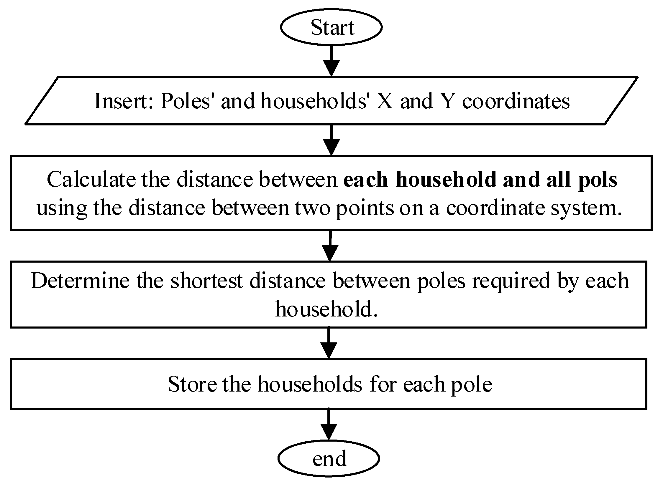
2.1.1. Shortest Path

In low-voltage alternating current (LVAC) distribution systems, electricity is mostly distributed from a three-phase distribution transformer to households with single-phase or three-phase feeders along electrical poles and roads. The shortest path is a method that studies the design topology using a radial system and provides the shortest cable use for an LVAC distribution network [9]. The steps for designing this radial topology with the shortest cable length are outlined in a flowchart shown in Figure 2.

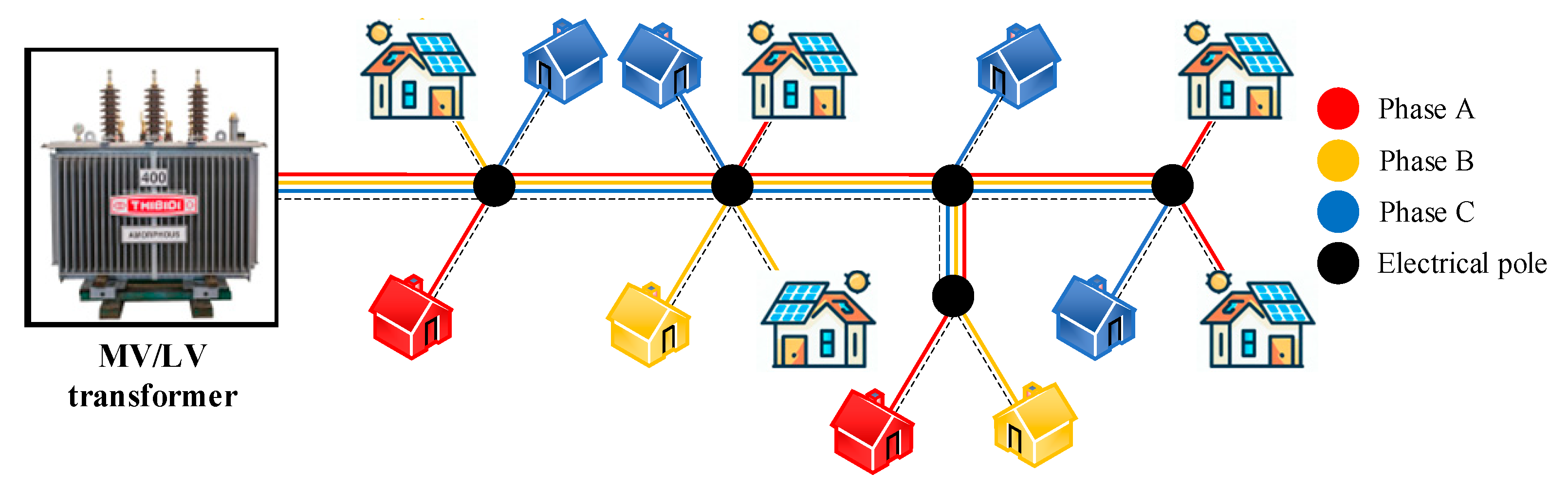
2.1.2. Power Phase Balancing

This part focuses on designing the structure of the LVAC distribution network by using the power phase balancing concept, and it provides two different cases of the research, such as Case 1 (pole balancing-PB) and Case 2 (load balancing-LB) as given in Figure 3 [10]. The objective of these cases is to minimize power loss while respecting voltage and current constraints using WCA for nonlinear optimization purposes [19].

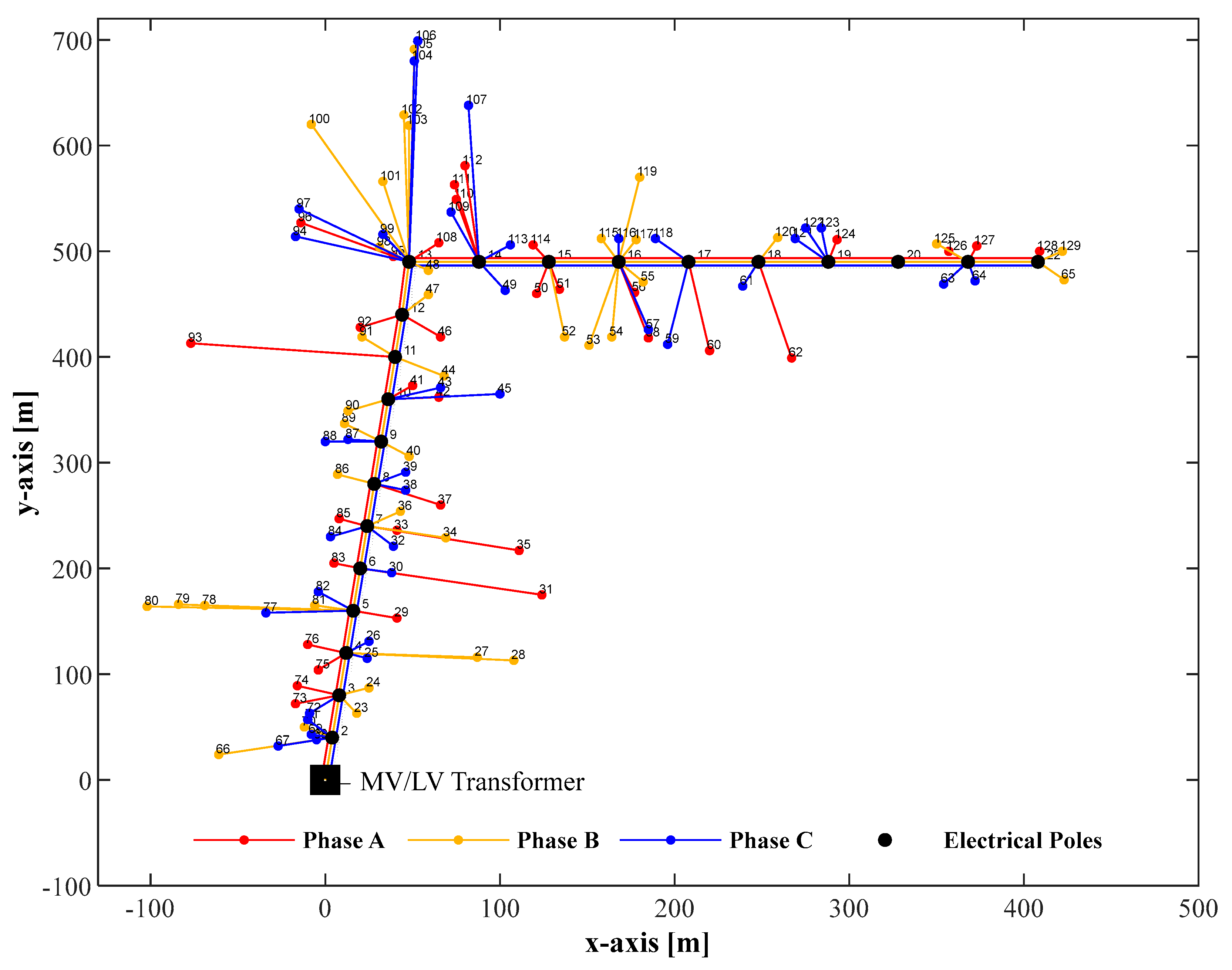
• Pole balancing (PB): in this case, the concept of single-phase connection of electrical poles is proposed by randomizing its phase connection (possible phase connection of electrical poles: Phase A, B, or C), which is performed using WCA optimization with the objective function of power loss.
• Load balancing (LB): focuses on random single-phases in households (it means that each household has selected the possible phase connections on Phases A, B, or C). It also has the same objective function as pole balancing and is implemented using WCA optimization.

2.1.3. Methods for Energy Loss Minimization

This point focuses on minimizing energy loss by proposing two different methods [20]. These methods are performed by taking into account a load profile to study the energy performance per day, and it is also implemented for the PB and LB concepts.

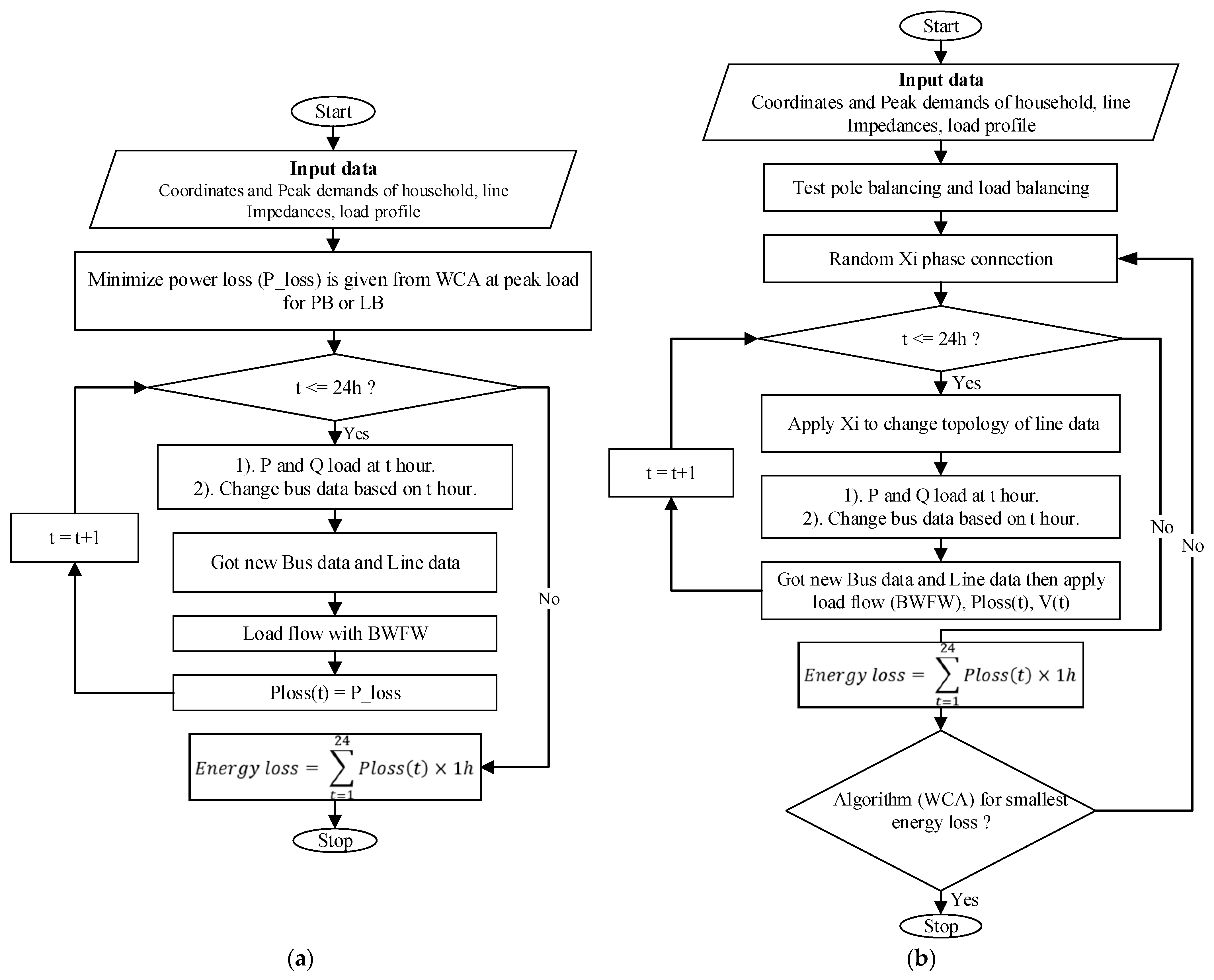
• Method 1: It investigates how to minimize power loss at peak load, and after that, a topology is given for PB and LB at peak load. Additionally, a load profile is performed on this method to attain the energy loss for a day. Figure 4a presents the process of Method 1 as a flow chart. Step 1 begins with the input of coordinates, peak demands of the household, line impedances, and a load profile. Step 2 involves choosing either case pole balancing or load balancing to simulate peak load in this step. Step 3 checks to see if the time is less than 24 h. Step 4 changes bus data based on its load profile. Step 5 obtains new bus data for a given period (t) in hours. Step 6 involves running backward-forward load flow to calculate power loss, voltage, and current. Step 6 then loops back to Step 2 until a certain condition is met. The final step involves calculating the energy loss.
• Method 2: It is a technique that focuses on reducing energy loss during the load profile of a power system using PB and LB to optimize the distribution and balancing of power. This can help to reduce energy costs and improve the efficiency of the power system. Figure 4b shows the flowchart for method 2, which is also used for both PB and LB. The first step involves inputting data such as coordinates (X, Y), peak household demands, line impedances (Z), and a load profile. The second step has case pole and load balancing and selects one to test in this method. The third step is a random phase connection (x) for 24 h. The fourth step focuses on testing LV topology for load profile and x-phase connection by performing load flow (BWFW) to obtain power loss, voltage profile, and current during each hour over 24 h. The fifth step provides a formula to calculate energy loss by summing the power loss of each hour and multiplying it by 1 h. Lastly, WCA optimization is performed to find the smallest energy loss until this condition is met.

2.1.4. PV System Installation

Integrating a PV installation into LVAC distribution networks can offer significant benefits in terms of reduced energy costs and environmental impact [21,22]. In this study, two concepts of PV integration are proposed: a centralized PV system, which is installed at MV/LV transformers (CePV), and a decentralized PV system (DePVs), which is installed on the rooftops of households and then integrates into the LV grid as given in Figure 5. In Cambodia, the policy is that the total size of PV systems that can be connected to the grid cannot exceed 50% of the transformer size or demand contract in kW [23], which is calculated by multiplying the kVA rating transformer by 0.9 (i.e., power factor). To figure out the size of the PV system, we need to know the transformer’s size in kW instead of kVA due to the power factor. For instance, if a transformer is 160 kVA, we can convert it to kW using a power factor of 0.9, resulting in a transformer size of 144 kW. Therefore, the size of the PV system that can be connected to the grid would need to be 72 kW, which is half of the transformer size in kW. To clarify, the total size of CePVs that can be installed is 72 kW, and the same total size of DePVs can also be installed. Since DePVs are installed in individual households, this study aims to use a water cycle algorithm (WCA) to optimize the location, size, and number of PV systems in the LVAC distribution network. This analysis is based on the voltage limit of each bus and power loss reduction to ensure that the PV systems operate efficiently and safely within the grid. Furthermore, in this section, we propose three scenarios for both CePV and DePV; which are zero injection to the grid; PV injection with no sell-back price; and PV injection with a sell-back price.

2.1.5. Water Cycle Algorithms (WCA)

In this study, the WCA is used to solve the problem formulation. The objective function and constraints were defined in the mathematical Equations provided in (1)–(3). However, since the analysis of this study is evaluated at the hourly level, short-term violations may exist for voltage and current at the minute level.

• Objective function

$$Objective=\min \left({\displaystyle \sum _{t=1}^{24h}{P}_{loss}\left(t\right)}\right)$$

(1)

• Subjective to:

$$0.9\le V_i\le 1.06$$

(2)

$$I_{line}\le I_{\max \_line}$$

(3)

where $P_{loss}$ is total active power loss in kW, $V_i$ is the voltage at $i$ bus in pu, $I_{line}$ is the current of each line in kA, and $I_{\max \_line}$ is the maximum current of each line in kA.

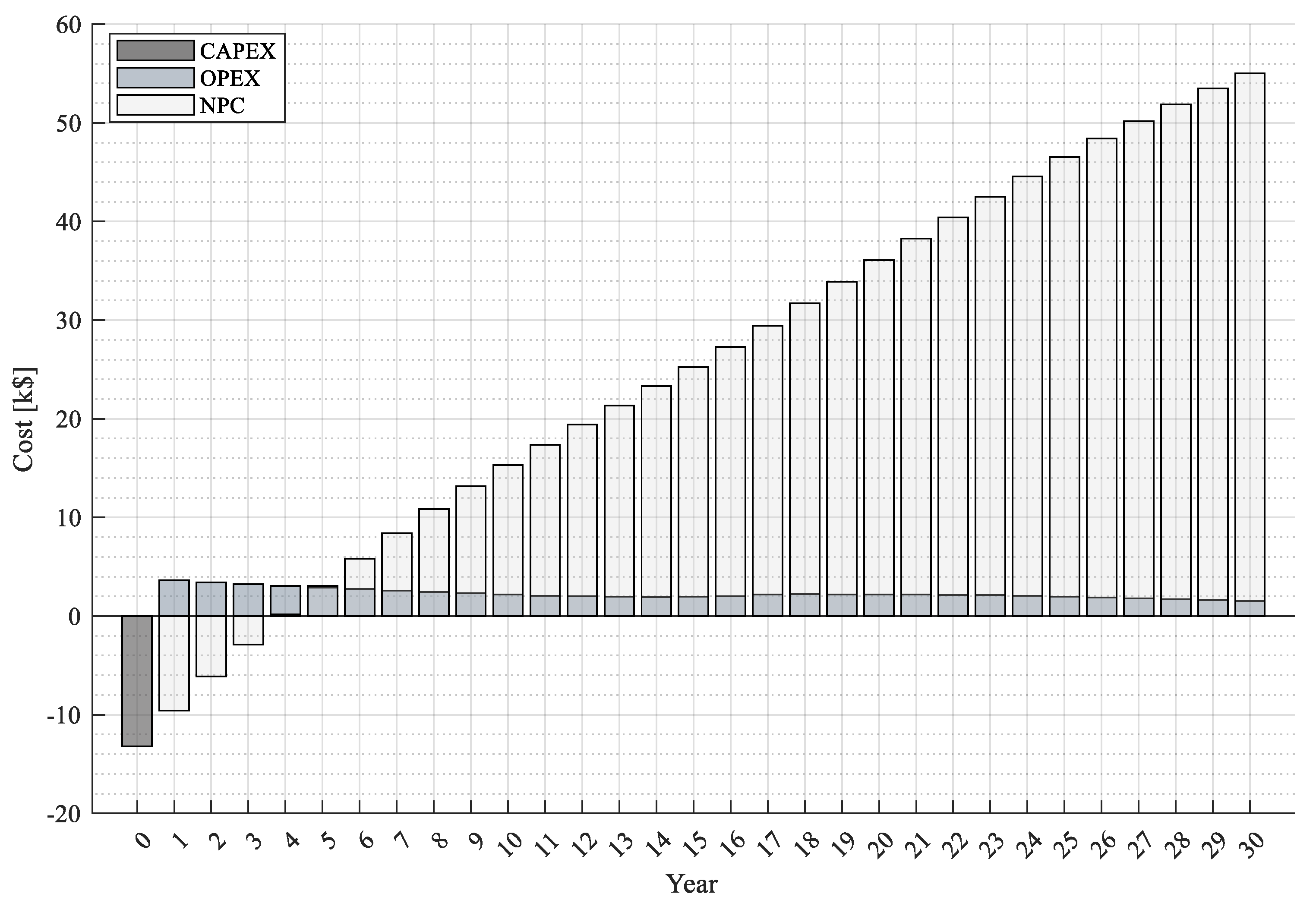
2.1.6. Economic Analysis

• CAPEX, OPEX, and NPC

This section presents the formulas used to measure the cost of the proposed method, including capital expenditure (CAPEX) and operating expenditure (OPEX) [3,4,24]. CAPEX stands for capital expenditure and includes the initial cost of acquiring and installing the equipment essential for the project, such as cables ($C_{cable}$), PV modules ($C_{PV}$), and PV inverters ($C_{inverter}$). It also covers the cost of replacing components ($C_{replacement}$), for example, the replacement cost of the inverter, which must be replaced after 15 years.

$$CAPEX=C_{cable}+C_{PV}+C_{inverter}+C_{replacement}$$

(4)

where $C_{cable}$ is the cost of total cable in k$, $C_{PV}$ is the cost of PV modules in k$, $C_{inverter}$ is the cost of inverter in k$, and $C_{replacement}$ is the cost of replacement in k$.

OPEX refers to the ongoing costs associated with operating and maintaining the system. It includes the cost of purchasing energy from the MV (medium voltage) grid as well as any costs related to selling energy to households and back to the grid from PV injection. O&M (operations and maintenance) costs, which include maintaining the PV components and other equipment that make up the system, are also included in OPEX.

$$OPEX={\displaystyle \sum _{T=1}^N\frac{\left(C_{EnergySold}-C_{EnergyPurchased}\right)\times 365-C_{O\&M}}{{\left(1+i\right)}^T}}$$

(5)

where $C_{EnergySold}$ is the cost of energy sold in k$, $C_{EnergyPurchased}$ is the cost of energy purchased in k$, $C_{O\&M}$ is the cost of operation and maintenance in k$, $i$ is the real discount rate [%], and $T$ is the index of the year.

The net present cost (NPC) equation is a way to calculate the total cost of a project or system, taking into account both the capital expenditure (CAPEX) and operating expenditure (OPEX). It helps project developers and investors evaluate a project’s financial viability. In short, the NPC equation is a crucial tool for assessing a project’s profitability and making informed decisions.

$$NPC=OPEX-CAPEX$$

(6)

• Real Discount Rate

The real discount rate is a percentage that shows how much future cash flows are worth today after accounting for inflation. The real discount rate is expressed as in (7).

$$i=\frac{i^{\prime }-f}{1+f}$$

(7)

where, $i^{\prime }$ is the nominal discount rate [%], and $f$ is the expected inflation rate [%].

2.1.7. Autonomous Operation Time, Energy, and CO₂ Emissions

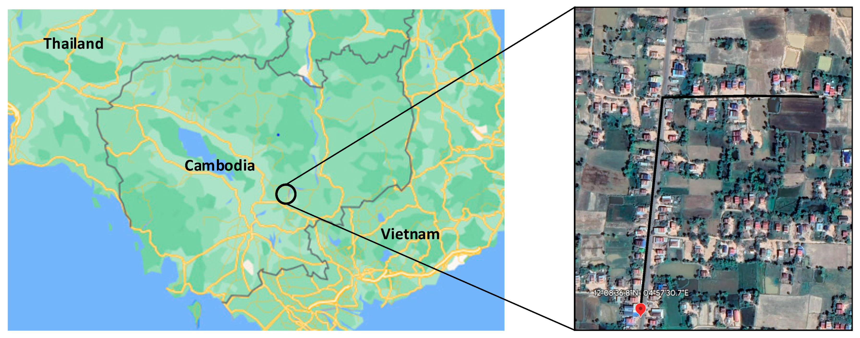
Grids are considered autonomous based on two factors [4]: (1) their ability to operate independently from the main grid for a certain amount of time (autonomous time expressed as a percentage (8)); and (2) the amount of energy they produce from their own solar panels compared to the total amount of energy needed by the main grid (autonomous energy expressed as a percentage (9)).

$$Autonomoustime(\%)=\frac{{\displaystyle \sum _{T=1}^N(Durationwithoutpowerfromthegridoverayear(T))}}{8760\times N}\times 100\%$$

(8)

$$Autonomousenergy(\%)=\frac{{\displaystyle \sum _{T=1}^N(TotalenergyproducedbyPVoverayear(T))}}{{\displaystyle \sum _{T=1}^N(Totalenergyneededbygridoverayear(T))}}\times 100\%$$

(9)

The total CO₂ emissions from energy use depend on how much carbon dioxide is released into the air when we generate and use energy, as provided by Equation (10) [4].

$$C{O}_{2}emissions(kg)={\displaystyle \sum _{i_{sources}=1}^{N_{sources}}LCC{O}_{2i_{sources}}\times E_{i_{sources}}}$$

(10)

where, $i_{sources}$ is an index of production types (i.e., one for PV and two for grid), $N_{sources}$ is the number of sources production types (i.e., two types), $LCC{O}_{2i_{sources}}$ is life-cycle CO₂ emissions in kg/kWh for source, and is the total energy produced from each source over the project in kWh.

2.2. Case Study

This study on low-voltage distribution systems selected a rural village in Sandek commune, Batheay district, Kampong Cham Province, Cambodia as shown in Figure 6 [9]. The village has a total of 22 electrical poles and 107 households. Electrical power is supplied using a 22/0.4-kV transformer with a capacity of 160 KVA placed at the first pole, with a total power of 43 kW in the initial year. The mainline and secondary lines have conductor sizes of 120 mm² and 4 mm², respectively. These details were used to model the low-voltage distribution system in the village and evaluate its performance.

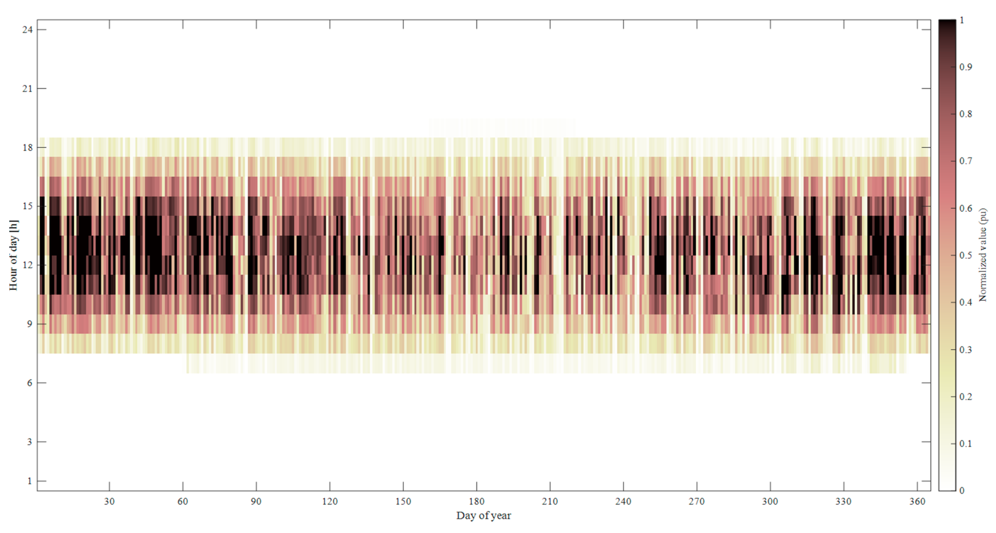
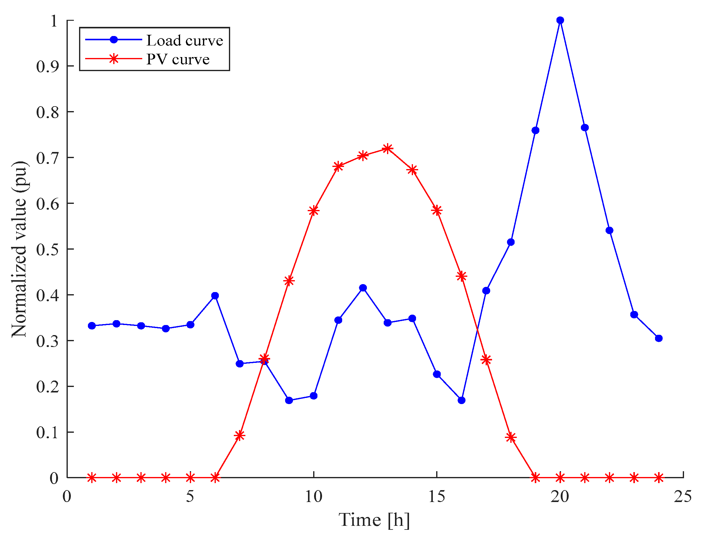
2.2.1. PV Curve and Load Curve

Figure 7 shows how much solar power was produced in p.u. over a year. This information came from software called HOMER Pro. The software used data from NASA for solar radiation [25]. Figure 8 was used to obtain a PV curve and a normalized load curve. The PV curve was determined by averaging the solar power generated over a year. The load curve at the site is based on the measurement using a power quality analyzer Fluke 435 series II. It is worth noting that these curves were assumed to remain constant during the planning period, which means that the same curves were used for simulations covering different periods (such as the 1st year, 2nd year, or up to the 30th year).

2.2.2. Tariff Payment for MV Feeders and Households in Rural Areas

Electricity is purchased from a medium voltage (MV) feeder and supplied to rural areas as part of this research study. Two different electricity tariffs between MV and LV are considered in this study; the distributor is paid based on monthly meter readings from the MV/LV transformer, and the households are charged a monthly payment for their electricity usage. This payment structure is designed to cover the costs of purchasing and distributing electricity while also ensuring that the electricity remains affordable and reliable for rural communities. The tariff rates for the distributor and household electricity usage in Cambodia are provided in

Table 1. The tariff of distributors based on MV consumer regulation as the hypothesis.

Description	MV Feeder
	General Tariff	PV Consumer
Capacity charge [$/kW/Month]	-	3.1
Tariff [$/kWh]	0.121	0.118

and

Table 2. The tariff on households.

Items	Provincial and Rural Areas
Electricity consumption [kWh/Month]	0–10	11–50	51–200	201–2000
Tariff [$/kWh]	0.095	0.12	0.1525	0.1825

, respectively, according to the relevant regulations [26].

2.2.3. Input Parameters

This section provides several input data used for simulating and analyzing the economic evaluation of the project.

Table 3. Input data.

Items	Value [Ref.]
Planning period [years]	30
Load growth [%]	3 [3]
Nominal discount rate [%]	12 [27]
Expected inflation rate [%]	3 [28]
Real discount rate [%]	8.74
PV price [k$/kWp]	0.6 [3]
PV lifetime [Years]	30 [3]
PV inverters [k$/kW]	0.556 [3]
Inverter lifetime [Years]	15 [3]
Inverter efficiency [%]	95 [3]
PV + inverter maintenance cost [k$/kW]	0.02 [3]
LV-2 × 4 mm2 [k$/km]	0.625
LV-ABC-4 × 120 mm2 [k$/km]	6.1
Life-cycle CO2 emissions of grid [kg/kWh]	0.400 [29]
Life-cycle CO2 emissions of CePV [kg/kWh]	0.042 [30]
Life-cycle CO2 emissions of DePV [kg/kWh]	0.066 [30]

[3,27,28,29,30] provides the input parameters, including load growth, the nominal discount rate, the expected inflation rate, the prices of PV panels, the prices of inverters, the prices of cables, etc. These data points are important for accurately modeling the financial performance of the project and assessing its economic viability over its expected lifetime [3,27,28]. Additionally, inputs of life-cycle CO₂ emissions for two types of sources (grid and PV) are provided in this section [29,30].

3. Simulation Results and Discussion

3.1. Optimal Radial Topology

In this study, four different strategies to build the LVAC distribution system for 30 years of operation were proposed. The costs and performance of each method were compared, and the results were presented in

Table 4. Test methods with pole balancing and load balancing.

Items	M1-PB	M1-LB	M2-PB	M2-LB
Transformer capacity [kVA]	160	160	160	160
Length of mainline (4 wires) [m]	852	852	852	852
Length of secondary (2 wires) [m]	5105	5105	5105	5105
Max. Voltage [pu]	1	1	1	1
Min. Voltage [pu]	0.905	0.906	0.908	0.910
Payback period [Year. Month]	3.652	3.635	3.643	3.634
Total energy loss [MWh]	202.421	189.958	195.471	189.274
Energy purchased [MWh]	7438.712	7426.248	7431.762	7425.564
Cost of energy purchased [k$]	900.084	898.576	899.243	898.493
CO2 emissions [tons]	2975.485	2970.499	2972.705	2970.226
CAPEX [k$]	13.197	13.197	13.197	13.197
OPEX [k$]	67.815	68.180	68.018	68.199
NPC [k$]	54.619	54.983	54.821	55.003

. The best method for a radial power system was found to be M2-LB (method two load balancing). It was found that this method has the highest NPC of 55.003 k$, including the OPEX of 68.199 k$. Additionally, it was observed that this method performs well in terms of energy loss (189.274 MWh), energy purchased (7425.564 MWh), minimum voltage of 0.910 pu, and CO₂ emissions of 2970.226 tons. Therefore, the M2-LB method is the most effective and efficient way to build the LVAC radial topology, as in this case study.

Figure 9 shows the cash flow for the M2-LB method. It displays the costs for CAPEX, OPEX, and NPC for each year. From the first to the third year, the NPC cost is negative, which means the project needs to spend money during these years. However, from the fourth to the thirtieth year, the NPC is positive, which means the project generates profit during these years.

In Figure 10, the best topology for radial topology and power phase balancing is shown using the M2-LB method. This method ensures that each household’s phase connection follows the load-balancing concept.

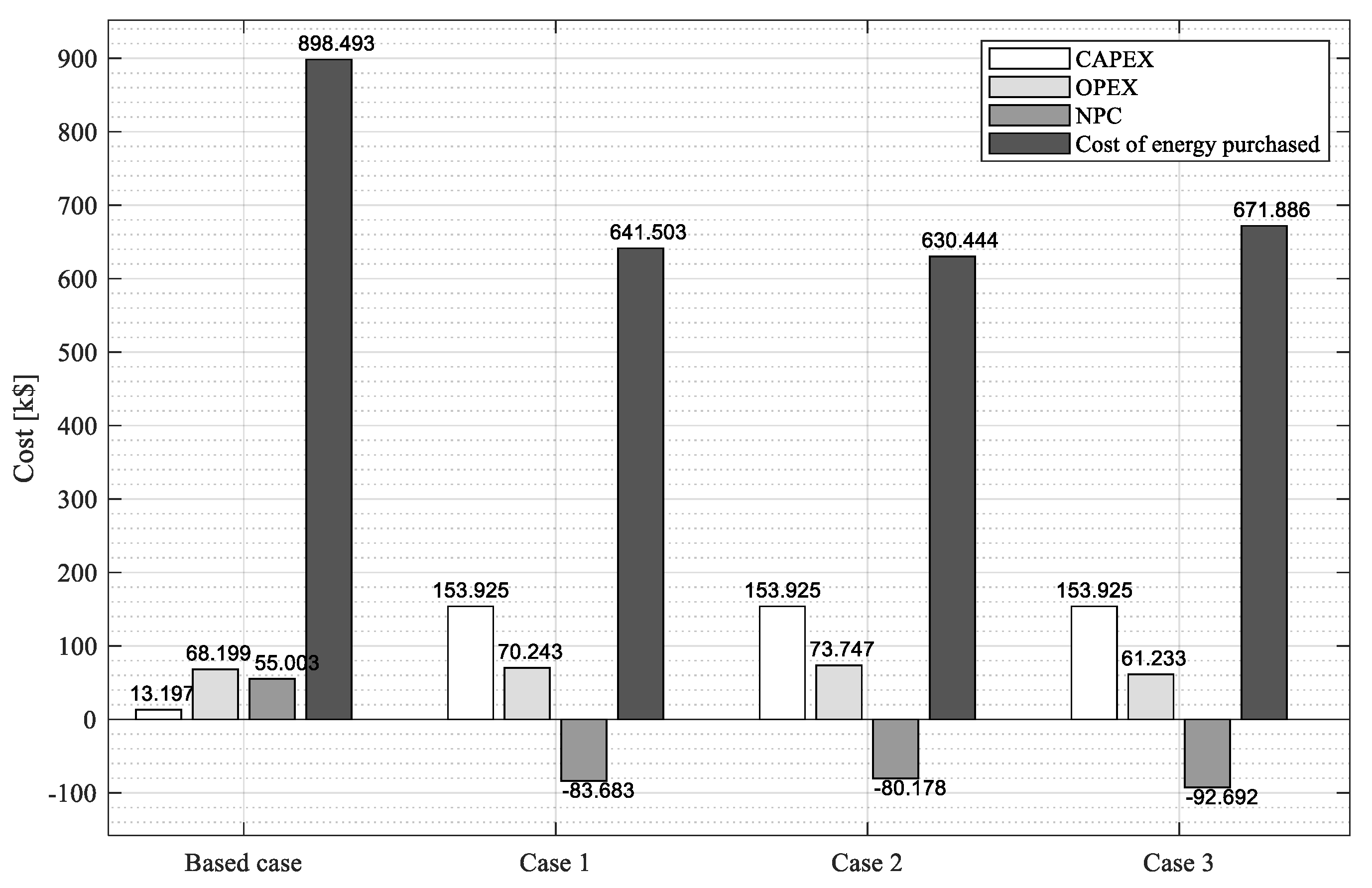
3.2. CePV and DePV Integration

3.2.1. Scenario 1: Zero Injection

The information presented in

Table 5. Comparison of PV installation with zero injection into the grid.

Items	Base Case	Case 1	Case 2	Case 3
PV capacity per HH [kWp]	-	-	0.828	0.828
Number of PV	-	-	87	87
Total PV capacity [kWp]	-	72	72	72
Max. Voltage [pu]	1	1	1	1
Min. Voltage [pu]	0.910	0.910	0.910	0.910
Payback period [Year. Month]	3.634	-	-	-
Total energy loss [MWh]	189.274	184.948	162.007	157.673
Energy purchased [MWh]	7425.564	5301.675	5210.281	5552.774
PV produced [MWh]	-	2119.563	2188.016	1841.189
Cost of energy purchased [k$]	898.493	641.503	630.444	671.886
CAPEX [k$]	13.197	153.925	153.925	153.925
OPEX [k$]	68.199	70.243	73.747	61.233
NPC [k$]	55.003	−83.683	−80.178	−92.692
Autonomous energy [%]	-	29	30	25
CO2 emissions [tons]	2970.226	2254.939	2168.381	2292.357
CO2 emissions reduction [%]	-	24	27	23

shows the results of the zero-injection grid scenario, comparing different cases such as the base case without PV (i.e., M2-LB), Case 1 with a CePV zero injection MV grid, Case 2 with a DePV zero injection MV grid, and Case 3 with a DePV zero injection LV grid. The table indicates that the base case without PV has the highest NPC of 55.003 k$, which means it is the most cost-effective system among all the cases studied. Therefore, the topology without PV is the best option for this particular scenario of zero injection.

For PV integration, Case 2, which involves autonomous operation using solar energy, displays the best system in terms of energy and CO₂ emission reductions compared to Case 1 and Case 3. This means the system performs better when it can operate autonomously using solar energy, resulting in lower CO₂ emissions.

Figure 11 displays the cost of each case, which has CAPEX, OPEX, NPC, and the cost of energy purchased. The base case has lower CAPEX and OPEX costs than Cases 1, 2, and 3. However, the base case has a profit with a higher NPC of $55.003 k$ compared to Cases 1, 2, and 3. In addition, the base case spends the most money on purchasing energy, with a cost of 898.493 k$, compared to Cases 1, 2, and 3.

3.2.2. Scenario 2: Injection to the MV Grid without Sell-Back Price

Table 6. Perform PV injection to the MV grid (no sell-back price).

Items	Base Case	Case 1	Case 2
PV capacity per HH [kWp]	-	-	0.828
Number of PV	-	-	87
Total PV capacity [kWp]	-	72	72
Max. Voltage [pu]	1	1	1
Min. Voltage [pu]	0.910	0.910	0.910
Payback period [Year. Month]	3.634	-	-
Total Energy loss [MWh]	189.274	188.758	252.045
Energy purchased [MWh]	7425.564	5187.568	5177.661
PV produced [MWh]	-	4350.979	4350.979
Energy injects to MV grid [MWh]	-	2113.498	2040.305
Cost of energy purchased [k$]	898.493	627.696	626.497
CAPEX [k$]	13.197	125.341	125.341
OPEX [k$]	68.199	79.457	79.740
NPC [k$]	55.003	−45.884	−45.601
Autonomous time [%]	-	36	36
Autonomous energy [%]	-	59	59
CO2 emissions [tons]	2970.226	2362.192	2253.805
CO2 emissions reduction [%]	-	20	24

presents the results of scenario 2, which includes three different cases: the base case without PV, Case 1 with CePV, and Case 2 with DePV. This study concludes that the base case without PV is the best scenario because it has the highest NPC of 55.003 k$ compared to the other scenarios. This suggests that for this particular LVAC distribution network, the most cost-effective option is to not use solar power and stick with the base case.

For PV integration, both Case 1 and Case 2 provide the same percentage of autonomous operation time and energy at 36% and 59%, respectively. However, Case 2 shows better CO₂ emission reductions than Case 1 and the base case, indicating that the system performs better when it can operate autonomously and results in lower CO₂ emissions.

In Figure 12, the costs of CAPEX, OPEX, NPC, and energy purchases for each case are presented. The base case shows lower CAPEX and OPEX expenses compared to Cases 1 and 2. However, it has a profile with a higher NPC of 55.003 k$ than Cases 1 and 2. Additionally, the base case incurs the highest cost for purchasing energy, totaling 898.493 k$.

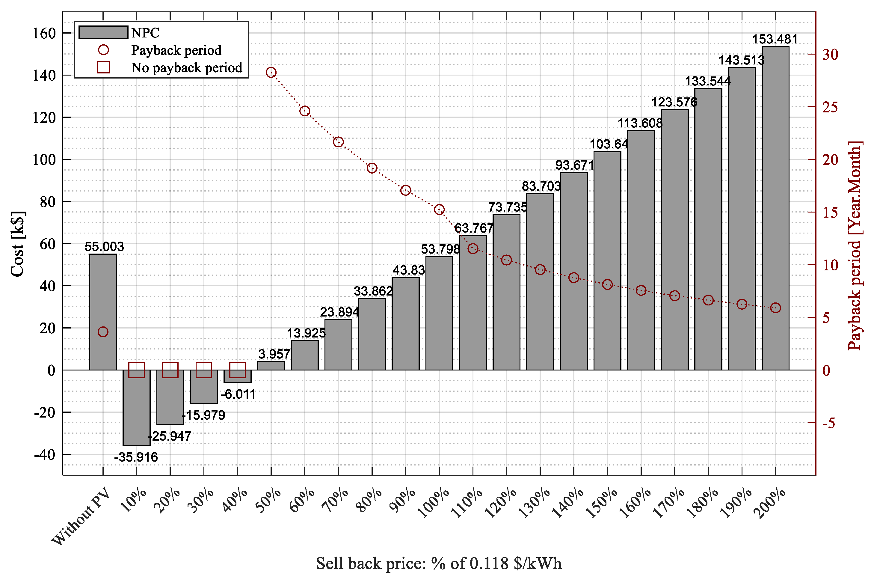
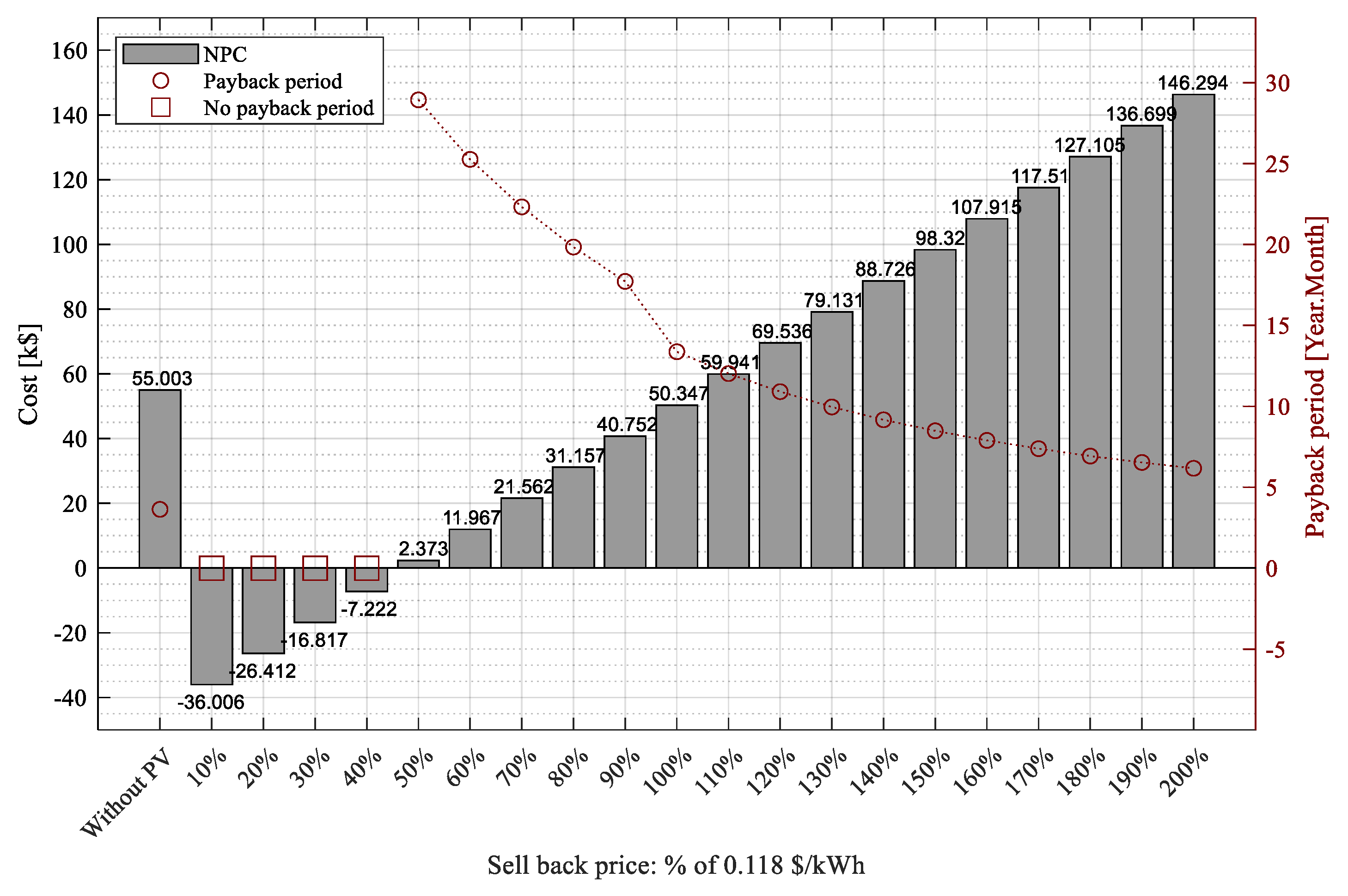
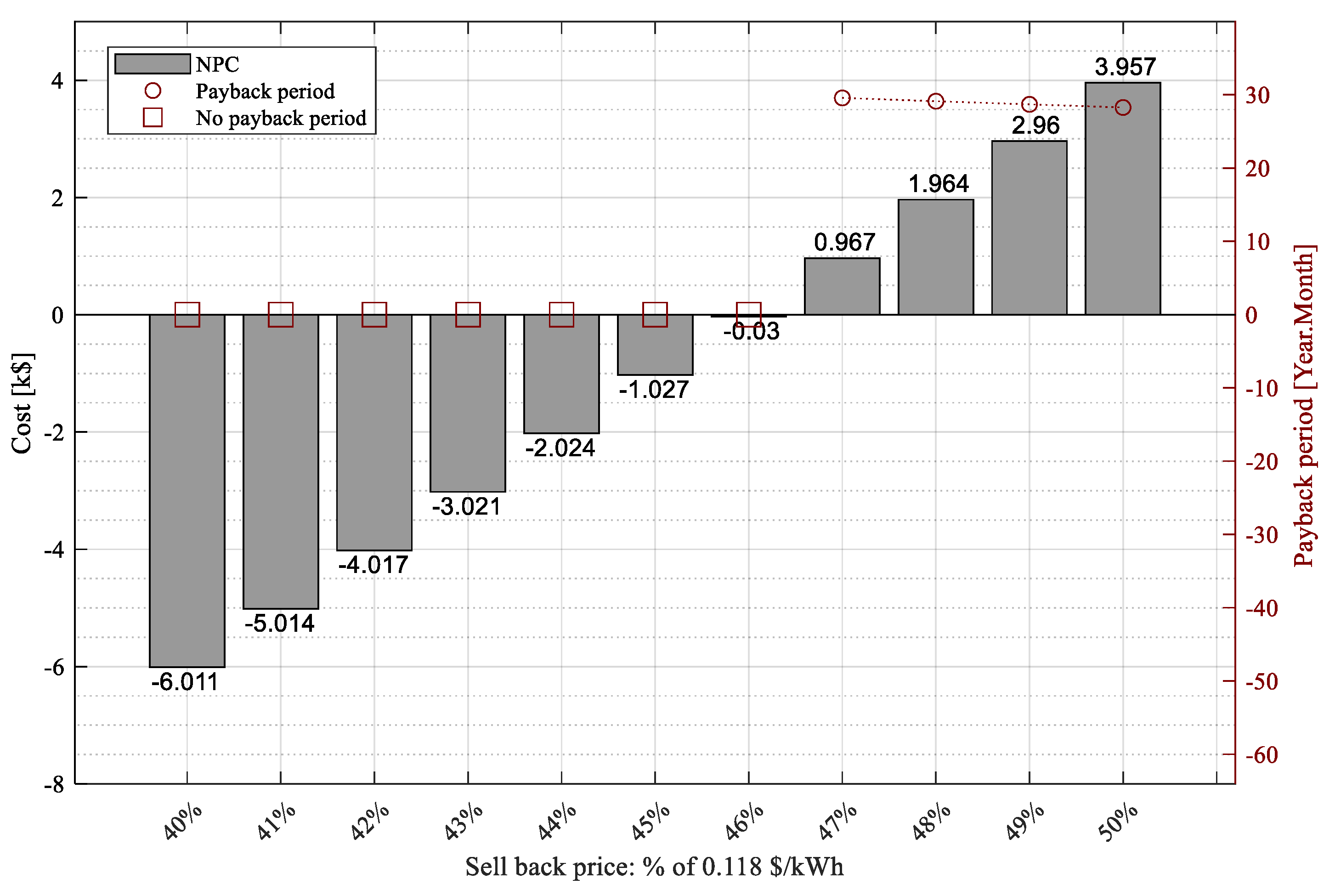
3.2.3. Scenario 3: Injection to the MV Grid with Sell-Back Price

• Strategy 1: Finding the sell-back price to get the profit

Figure 13 shows a bar graph comparing the cost of NPC and the payback period with and without CePV. CePV proposes that the sell-back price start at 10% to 200% of 0.118 $/kWh. For an explanation of the figure, as the sell-back price increases, the value of NPC also increases while the payback period decreases, as shown in the graph. To be profitable with CePV integration, compared to the NPC of topology without PV, the price of selling back electricity must be more than 110% of the price of buying electricity from the power grid ($0.118 per kWh), and the payback period starts at 11.5 years and decreases from there.

Figure 14 has a graph comparing the NPC and payback period without PV and with DePV. DePV studies selling electricity back at a price starting at 10% to 120% of 0.118 $/kWh. To make a profit with DePV integration, compared to the NPC of topology without PV, the selling price of electricity needs to be at least 110% higher than the cost of buying electricity from the power grid, and the payback period is decremented starting from 12 (year, month).

• Strategy 2: Minimize the sell-back price to get the profit

Figure 15 is a graph that displays the NPC and payback period of the CePV system at different sell-back prices. The graph demonstrates that for the CePV system to make a profit, it needs to sell the cost of electricity back to the grid at a price higher than 47% of the cost it pays to buy electricity from the grid, and the payback period decreases from a value of 29.6 (year, month), which is $0.118 per kWh.

Figure 16 shows the graph of the NPC and payback period of DePV with the proposed percentage of the sell-back price. To make a profit, DePV needs to sell the cost of electricity back to the grid at a price higher than 48% of the cost it pays to buy electricity from the grid (which is $0.118 per kWh), and the payback period is decremented starting from 29.8 (year, month).

To summarize, the first strategy, CePV and DePV, both need to sell electricity back at 110% of 0.118 $/kWh to make a profit compared to the NPC of the topology without PV. However, the second strategy shows that CePV is better than DePV because it has a lower sell-back price, starting at 47%. This means that investing in CePV gives a better return compared to investing in DePV. After simulation, notice that as the sell-back price increases, the value of NPC also increases while the payback period decreases.

4. Conclusions

This research study compares different topologies with and without PV integration in rural areas of Cambodia over 30 years. The different radial topologies are evaluated and compared based on the shortest path method for minimizing cable length. Pole and load balancing techniques are developed to minimize power losses, improve voltage, and simulate methods for minimizing energy loss over 24 h. With a radial topology and phase power balancing, Method 2 with load balancing (M2-LB) has the highest NPC and is the best approach for radial topology. The study of systems with and without PV (CePV and DePV) integration into the optimal radial topology is also investigated; Scenario 1 is for zero injection into the grid, with three cases: CePV with zero injection into MV grid, DePV with zero injection to the MV grid, and DePV with zero injection to the LV grid. With this scenario, the base case is the highest NPC for the LVAC distribution network. Scenario 2 has three cases; PV injection into the MV grid without a sell-back price, and the base case without PV integration is the best case with the highest NPC. Next, Scenario 3 has two sell-back price strategies. Strategy 1 compares the topology without PV to the topology with PV to find the sell-back price to profit from CePV and DePV; upon comparing a topology without PV, the sell-back price should be at least 110% of 0.118 $/kWh. Strategy 2: Find the minimal sell-back price for CePV and DePV, in which the minimum sell-back price is also provided, which has the minimum sell-back price of 47% and 48% of 0.118 $/kWh for the cases of CePV and DePV, respectively, to generate profit from the project. In addition, autonomous operation and environmental indications are also provided. In conclusion, this study provides a planning tool for an effective economic analysis considering CAPEX, OPEX, NPC, voltage improvement, and environmental indicators in the LVAC distribution network with DePV-CePV integration. However, the integration of PV and storage into the low-voltage distribution system will be investigated in future work.

References

1. Akinyemi, A.; Musasa, K.; Davidson, I. Analysis of voltage rise phenomena in electrical power network with high concentration of renewable distributed generations. Res. Sq. 2022, 12, 7815. [Google Scholar] [CrossRef] [PubMed]
2. Al-Jaafreh, M.A.A.; Mokryani, G. Planning and operation of LV distribution networks: A comprehensive review. IET Energy Syst. Integr. 2019, 1, 133–146. [Google Scholar] [CrossRef]
3. Chhlonh, C.; Alvarez-Herault, M.C.; Vai, V.; Raison, B. Comparative planning of LVAC for microgrid topologies with PV-storage in rural areas—Cases study in Cambodia. In Proceedings of the 2022 IEEE PES Innovative Smart Grid Technologies Conference Europe, Novi Sad, Serbia, 10–12 October 2022; pp. 1–5. [Google Scholar]
4. Khon, K.; Chhlonh, C.; Vai, V.; Alvarez-Herault, M.C.; Raison, B.; Bun, L. Comprehensive low voltage microgrid planning methodology for rural electrification. Sustainability 2023, 15, 2841. [Google Scholar] [CrossRef]
5. Vai, V.; Bun, L. Study on the impact of integrated PV uncertainties into an optimal LVAC topology in a rural village. ASEAN Eng. J. 2020, 10, 79–92. [Google Scholar] [CrossRef]
6. Eth, O.; Vai, V.; Bun, L.; Eng, S.; Khon, K. Optimal radial topology with phase balancing in LV distribution system considering energy loss reduction: A case study in Cambodia. In Proceedings of the 2022 4th International Conference on Electrical, Control and Instrumentation Engineering (ICECIE), Kuala Lumpur, Malaysia, 26 November 2022; pp. 1–6. [Google Scholar]
7. Jimenez, V.A.; Will, A.L.E.; Lizondo, D.F. Phase reassignment for load balance in low-voltage distribution networks. Int. J. Electr. Power Energy Syst. 2022, 137, 107691. [Google Scholar] [CrossRef]
8. Homaee, O.; Mirzaei, M.J.; Najafi, A.; Leonowicz, Z.; Jasinski, M. A practical probabilistic approach for load balancing in data-scarce LV distribution systems using discrete PSO and 2 m + 1 PEM. Int. J. Electr. Power Energy Syst. 2021, 135, 107530. [Google Scholar] [CrossRef]
9. You, L.; Vai, V.; Eam, D.; Hem, P.; Heang, S.; Eng, S. Optimal topology of LVAC in a rural village using Water Cycle Algorithms. In Proceedings of the 2022 IEEE International Conference on Power Systems Technology (POWERCON), Kuala Lumpur, Malaysia, 12–14 September 2022; pp. 1–5. [Google Scholar]
10. Eam, D.; Vai, V.; You, L.; Hem, P.; Heang, S.; Eng, S. Phase balancing improvement in unbalanced MV distribution systems. In Proceedings of the 2022 19th International Conference on Electrical Engineering/Electronics, Computer, Telecommunications and Information Technology (ECTI-CON), Prachuap Khiri Khan, Thailand, 24–27 May 2022; pp. 1–4. [Google Scholar]
11. Ibraheem, W.E.; Gan, K.C.; Mohd, M.R. Impact of photovoltaic (PV) systems on distribution networks. Int. Rev. Model. Simul. 2014, 7, 298–310. [Google Scholar]
12. Dinh, B.H.; Nguyen, T.T.; Nguyen, T.T.; Pham, T.D. Optimal location and size of photovoltaic systems in high voltage transmission power networks. Ain Shams Eng. J. 2021, 12, 2839–2858. [Google Scholar] [CrossRef]
13. Montoya, O.D.; Grisales-Noreña, L.F.; Giral-Ramírez, D.A. Optimal placement and sizing of PV sources in distribution grids using a Modified Gradient-Based Metaheuristic Optimizer. Sustainability 2022, 14, 3318. [Google Scholar] [CrossRef]
14. Dakić, P.; Kotur, D. Optimal placement of PV systems from the aspect of minimal power losses in distribution network based on genetic algorithm. Therm. Sci. 2018, 22, 1157–1170. [Google Scholar] [CrossRef]
15. Thapar, S. Centralized vs decentralized solar: A comparison study (India). Renew. Energy 2022, 194, 687–704. [Google Scholar] [CrossRef]
16. Husein, M.; Chung, I.Y. Optimal design and financial feasibility of a university campus microgrid considering renewable energy incentives. Appl. Energy 2018, 225, 273–289. [Google Scholar] [CrossRef]
17. Sackey, D.M.; Amoah, M.; Jehuri, A.B.; Owusu-Manu, D.G.; Acapkovi, A. Techno-economic analysis of a microgrid design for a commercial health facility in Ghana- Case study of Zipline Sefwi-Wiawso. Sci. Afr. 2023, 19, e01552. [Google Scholar] [CrossRef]
18. Sharma, S.; Sood, Y.R.; Sharma, N.K.; Bajaj, M.; Zawbaa, H.M.; Turky, R.A.; Turky, S. Modeling and sensitivity analysis of grid-connected hybrid green microgrid system. Ain Shams Eng. J. 2022, 13, 101679. [Google Scholar] [CrossRef]
19. Sadollah, A.; Eskandar, H.; Lee, H.K.; Yoo, D.G.; Kim, J.H. Water cycle algorithm: A detailed standard code. SoftwareX 2016, 5, 37–43. [Google Scholar] [CrossRef]
20. Eam, D.; Vai, V.; Eng, S.; You, L. Optimizing phase allocation arrangement for a rural lvac distribution system: A case study in Cambodia. In Proceedings of the 2022 4th International Conference on Electrical, Control and Instrumentation Engineering (ICECIE), Kuala Lumpur, Malaysia, 26 November 2022; pp. 1–6. [Google Scholar]
21. Uzum, B.; Onen, A.; Hasanien, H.M.; Muyeen, S.M. Rooftop solar PV penetration impacts on distribution network and further growth factors—A comprehensive review. Electronics 2021, 10, 55. [Google Scholar] [CrossRef]
22. Karimi, M.; Mokhlis, H.; Naidu, K.; Uddin, S.; Bakar, A.H.A. Photovoltaic penetration issues and impacts in distribution network—A review. Renew. Sustain. Energy Rev. 2016, 53, 594–605. [Google Scholar] [CrossRef]
23. EAC. Report on the Decision on Setting the Price List for Electricity for all Types of Consumers Who Buy Electricity from the Substation and from the Distribution Network Originates from the National Network of Private Electricity Suppliers for 2023; Electricity Authority of Cambodia: Phnom Penh, Cambodia, 2023. Available online: https://www.eac.gov.kh/document/tariffdecidelist (accessed on 12 June 2023).
24. Vai, V.; Alvarez-Herault, M.C.; Raison, B.; Bun, L. Optimal low-voltage distribution topology with integration of pv and storage for rural electrification in developing countries: A case study of Cambodia. J. Mod. Power Syst. Clean Energy 2020, 8, 531–539. [Google Scholar] [CrossRef]
25. NASA. ASDC Processing, Archiving, and Distributing Earth Science Data; NASA Langley Research Center (LaRC): Hampton, VA, USA, 2023. Available online: https://eosweb.larc.nasa.gov/ (accessed on 12 June 2023).
26. EAC. Salient Features of Power Development in the Kingdom of Cambodia in 2022; Electricity Authority of Cambodia: Phnom Penh, Cambodia, 2022. Available online: https://www.eac.gov.kh/site/annualreport?lang=en (accessed on 31 December 2022).
27. Vai, V.; Eng, S. Study of grid-connected PV system for a low voltage distribution system: A case study of Cambodia. Energies 2022, 15, 5003. [Google Scholar] [CrossRef]
28. ADB. Inflation Rate in Asia and the Pacific, Asian Development Outlook (ADO); Asian Development Bank/ERCD: Mandaluyong, Philippines, 2023; Available online: https://data.adb.org/dataset/inflation-rate-asia-and-pacific-asian-development-outlook (accessed on 4 April 2023).
29. Our World in Data. Carbon Intensity of Electricity. 2022. Available online: https://ourworldindata.org/grapher/carbon-intensity-electricity (accessed on 12 June 2023).
30. IPCC. Technology-Specific Cost and Performance Parameters; The Intergovernmental Panel on Climate Change (IPCC): Geneva, Switzerland, 2014; Available online: https://www.ipcc.ch/site/assets/uploads/2018/02/ipcc_wg3_ar5_annex-iii.pdf (accessed on 12 June 2023).
Figure 1. Flowchart of the proposed method.
Energies 16 05995 g001
Figure 2. Flowchart of shortest path method.
Energies 16 05995 g002
Figure 3. LV distribution topology using pole balancing (a) and load balancing (b).
Energies 16 05995 g003
Figure 4. Flow chart of Method 1 (a) and Method 2 (b).
Energies 16 05995 g004
Figure 5. LV distribution network with DePV installation.
Energies 16 05995 g005
Figure 6. Studied site in Batheay-Kampong Cham-Cambodia [12°08′36.8″ N,104°57′30.7″ E].
Energies 16 05995 g006
Figure 7. Heatmap of PV curve for 365 days.
Energies 16 05995 g007
Figure 8. Load and PV curve for simulation.
Energies 16 05995 g008
Figure 9. Cash flow of M2-LB algorithm.
Energies 16 05995 g009
Figure 10. Optimal radial topology by M2-LB algorithm.
Energies 16 05995 g010
Figure 11. The bar graph for the cost of scenario 1.
Energies 16 05995 g011
Figure 12. The bar graph for the cost of scenario 2.
Energies 16 05995 g012
Figure 13. Without PV vs. CePV with sell-back prices.
Energies 16 05995 g013
Figure 14. Without PV vs. DePV with sell-back prices.
Energies 16 05995 g014
Figure 15. CePV with sell-back prices.
Energies 16 05995 g015
Figure 16. DePV with sell-back prices.
Energies 16 05995 g016