
Comparative Study of Global Sensitivity Analysis and Local Sensitivity Analysis in Power System Parameter Identification


Abstract
:1. Introduction
2. Sensitivity Analysis Methods
2.1. Local Sensitivity Analysis Method
2.2. Global Sensitivity Analysis Method
2.2.1. Sobol Method
2.2.2. Morris Method
2.2.3. Regional Sensitivity Analysis Method
2.2.4. Scatter Plot Method
2.2.5. Andres Visualization Test Method
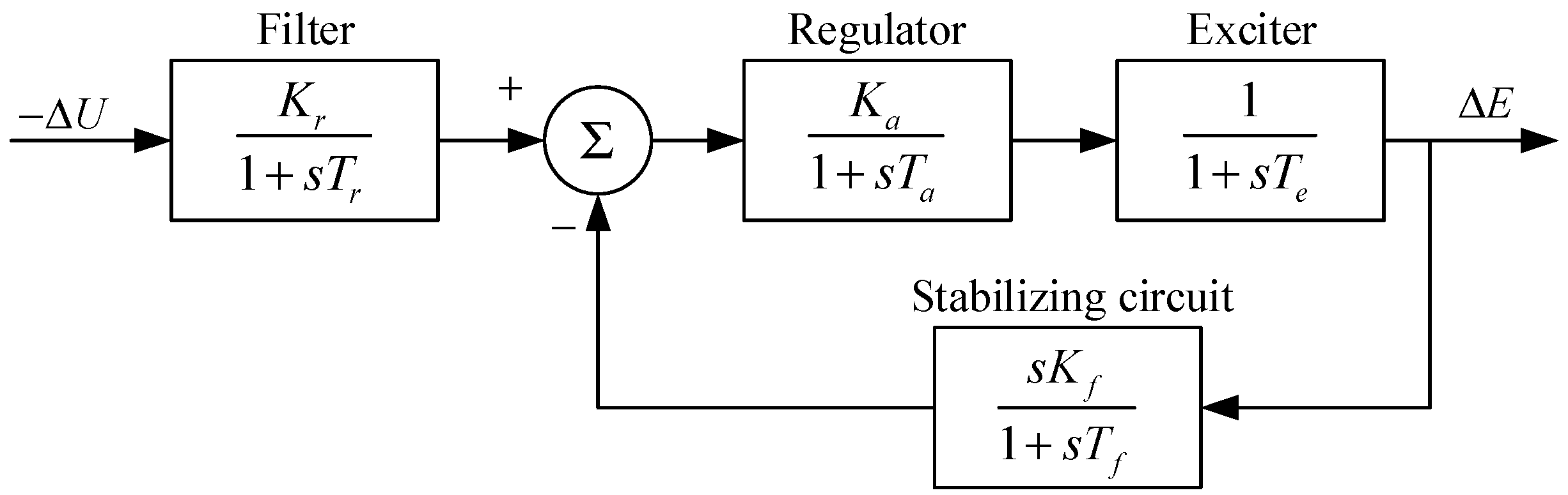
3. Model of Excitation System
4. Sensitivity Analysis Results
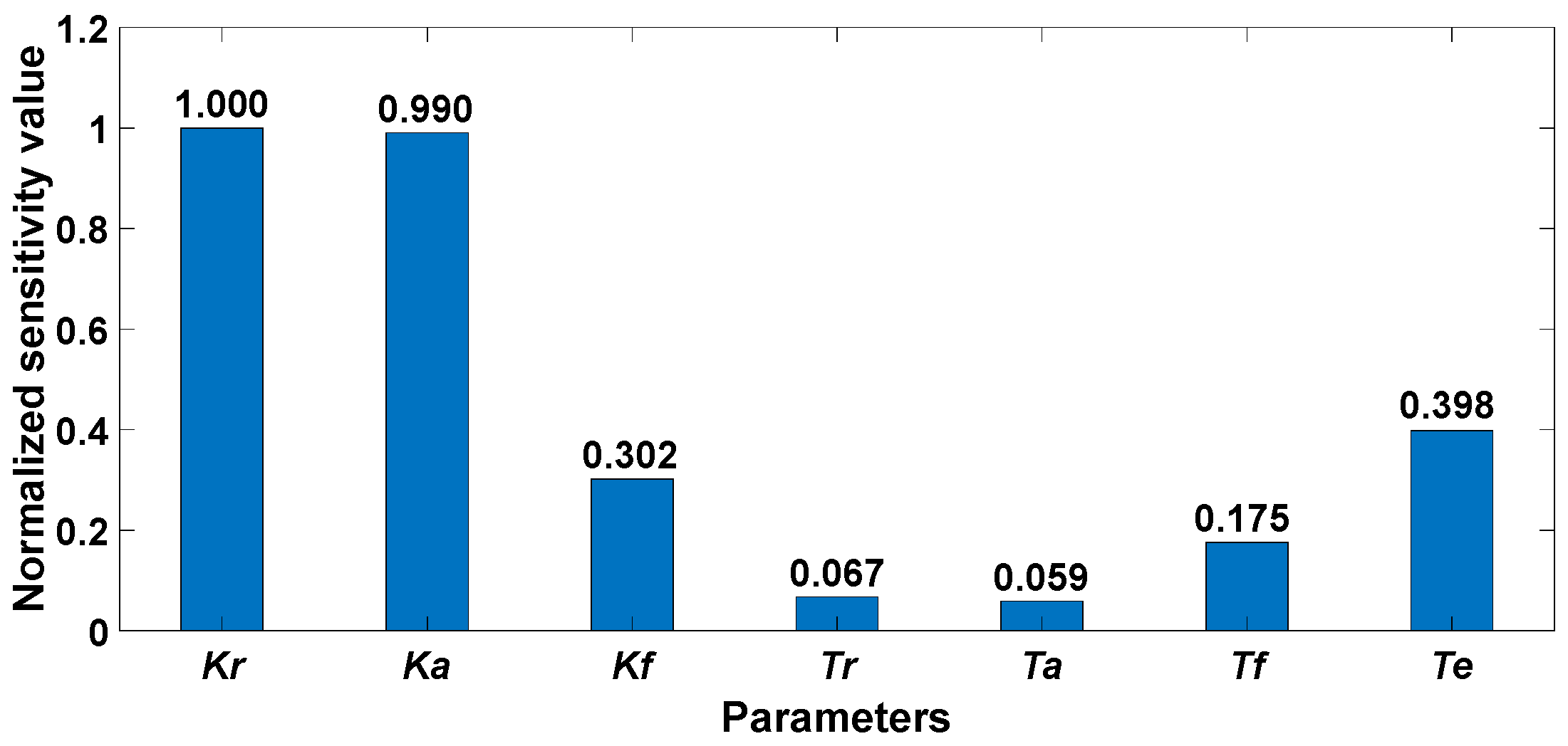
4.1. LSA Results
4.2. GSA Results
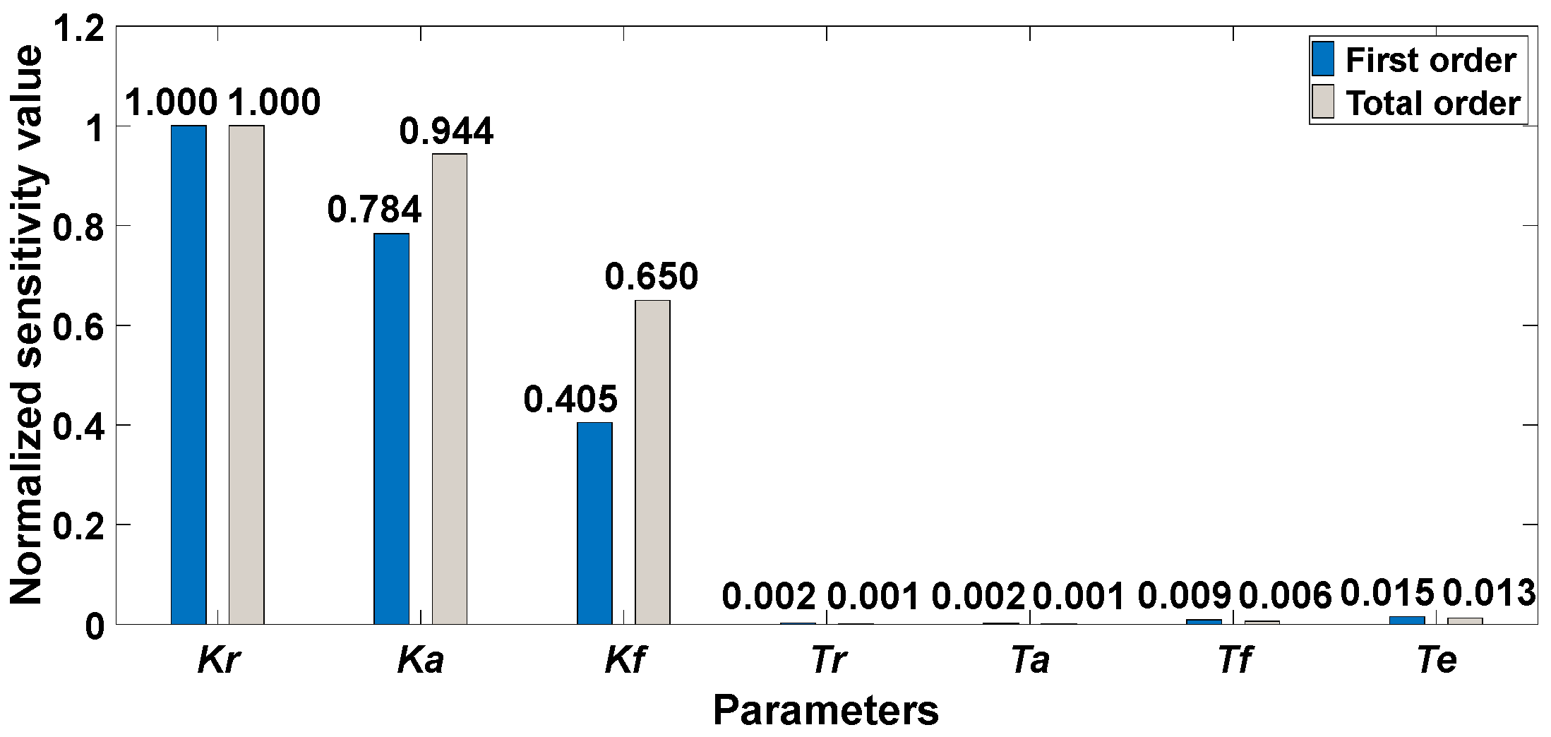
4.2.1. Sobol Method
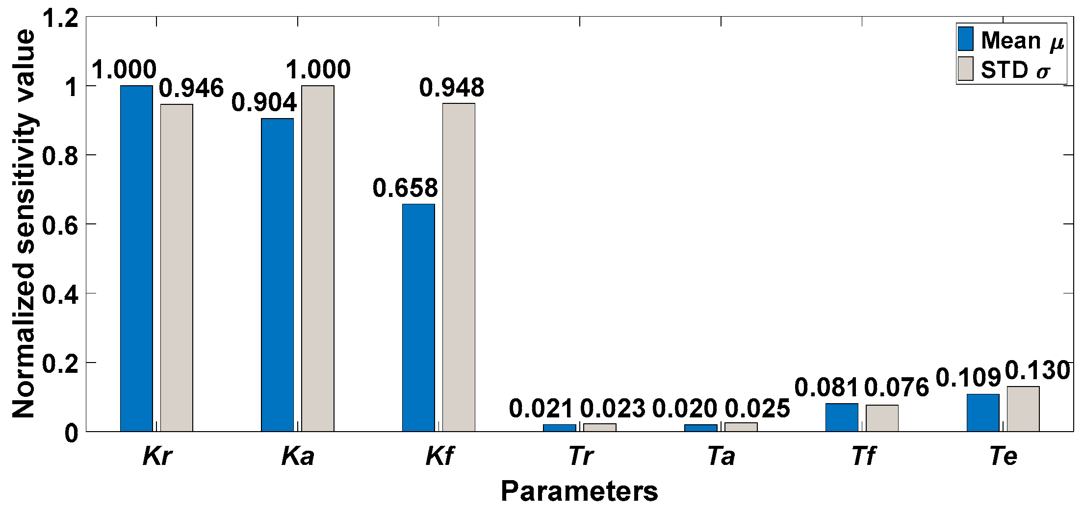
4.2.2. Morris Method
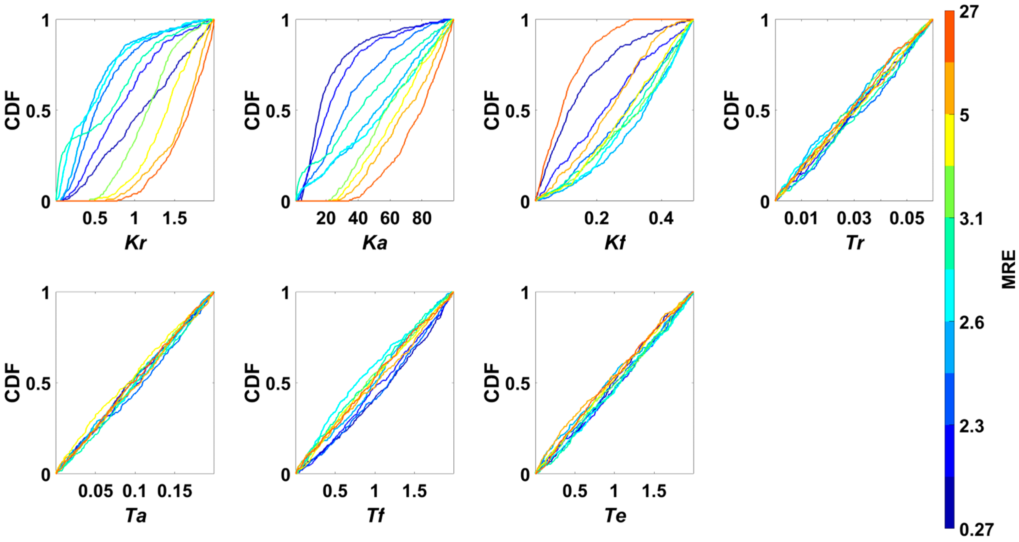
4.2.3. RSA Method
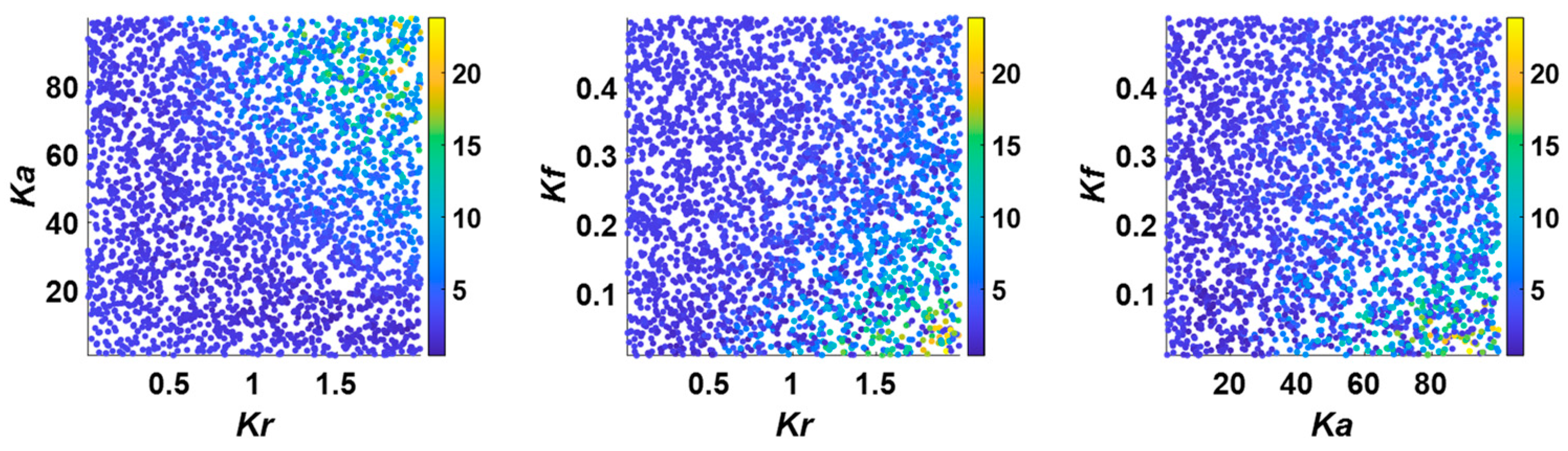
4.2.4. Scatter Plot Method
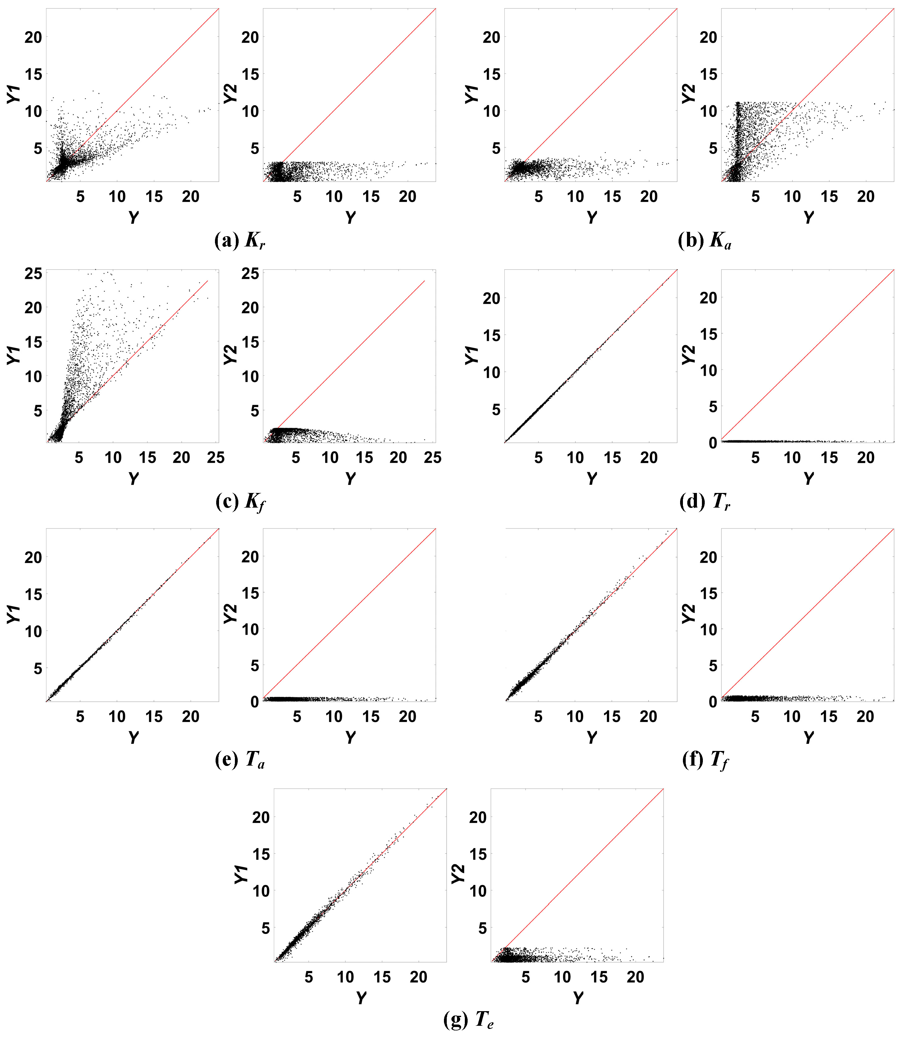
4.2.5. AVT Method
4.3. Comparison of the LSA and GSA Results
- In terms of the amount of calculation, the GSA is far more than that of LSA. The relationship between the number of times that various sensitivity analysis methods calculate the model output, the number of parameters N, and the number of parameter samples Ns is summarized in Table 4. If the single calculation of the model output is time-consuming, unless a suitable algorithm is found [52,53], the analysis speed of the GSA method may be unacceptable.
- Both LSA and GSA can be used to distinguish between key and non-key parameters. Although the LSA method and the numerical GSA method have the same parameter-sensitive ordering, the key parameters determined by the two kinds of methods are different. The key parameters in the LSA result are {Kr, Ka, Te, Kf, Tf}. When integrating the results of the five GSA methods, the key parameter is {Kr, Ka, Kf}. The reason is that the difference in parameter sensitivity is more significant in the GSA results, resulting in fewer key parameters being found.
- Although the analysis process and result display form of the five GSA methods are different, the conclusions are the same. Therefore, there is no need to use multiple GSA methods at the same time. Because the results of numerical methods are clearer and can be used to rank parameter sensitivity, we recommend the numerical GSA method.
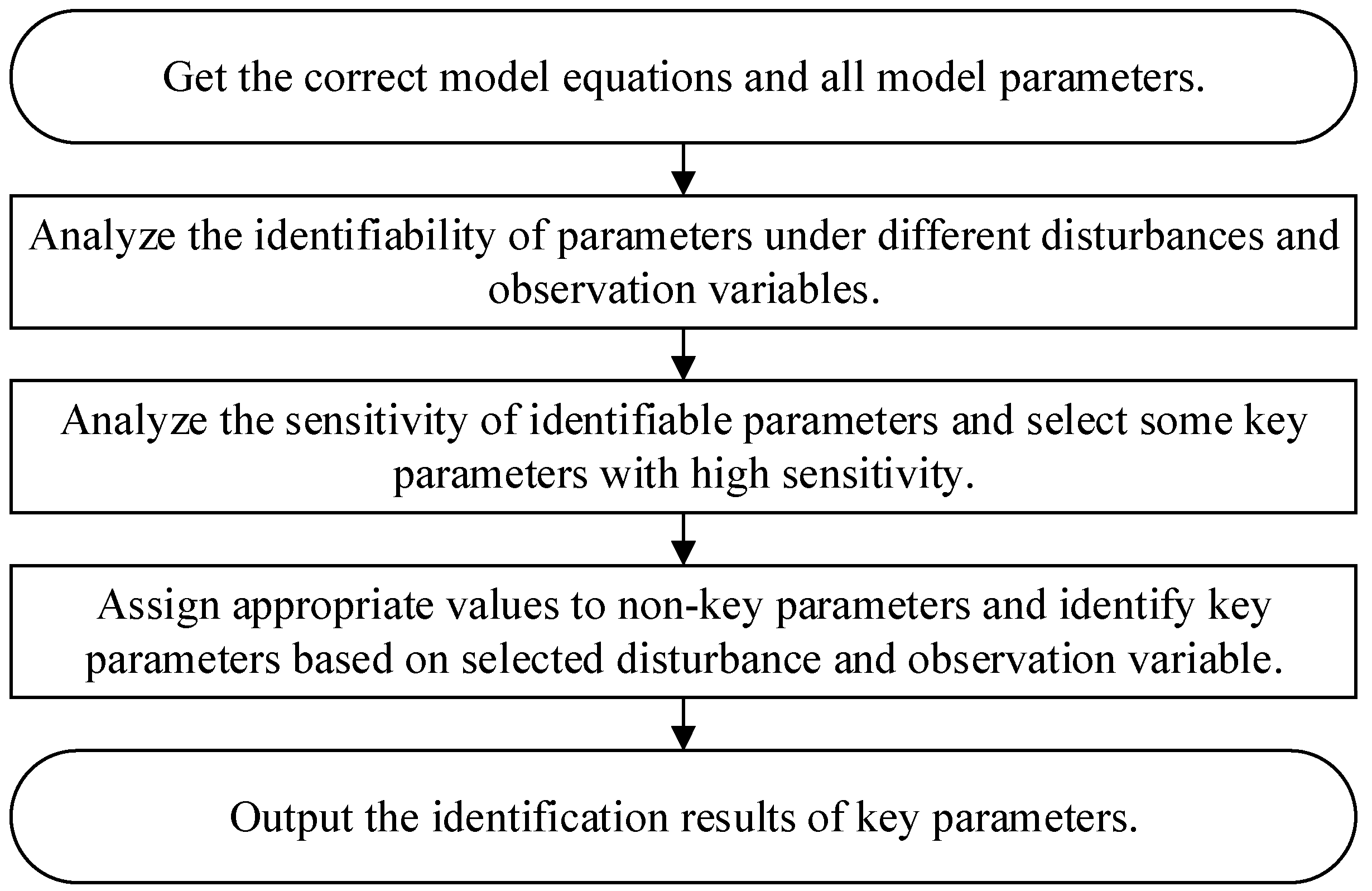
5. Comparison under Existing Parameter Identification Strategy
5.1. Identification Result According to LSA
5.2. Identification Result According to GSA
5.3. Example of High Sensitivity Not Equating to Identifiability
5.4. Discussion of the LSA-Based and GSA-Based Identification Results
6. Comparison under an Alternating Identification Strategy of High- and Low-Sensitivity Parameters
6.1. Process of the Alternating Identification
- Parameter identifiability analysis uses formula derivation or numerical methods [3] instead of the GSA methods. The identifiability analysis results in Section 3 and the sensitivity analysis results in Section 4 clearly show that the high sensitivity of the parameters does not mean that the parameters can be uniquely identified, such as three gain parameters Kr, Ka, and Kf.
- Sensitivity can be analyzed by LSA or GSA. The parameters are divided into only two groups, namely, the high-sensitivity parameter group and the low-sensitivity parameter group. The boundary of the grouping is 1/10 of the highest sensitivity value.
- The initial value of each parameter is obtained by identifying all the parameters at the same time once.
- Alternating identification starts from the low-sensitivity parameter group because, in the first identification of all parameters, the accuracy of the high-sensitivity parameter group is higher than that of the low-sensitivity parameter group.
- The random search of the PSO algorithm does not guarantee that each round of search can obtain a better fitting accuracy of the model output. Therefore, 10 opportunities are set for the identification of each parameter group. If the fitting error cannot be reduced within 10 identification iterations, the entire identification process ends.
- The expected final value of the fitting error is set to less than 0.01%.
- In the following comparison, when the GAIS can at least improve the identification accuracy of all key parameters, the identification is considered successful.
6.2. Application of LSA and GSA in the Alternate Identification Process
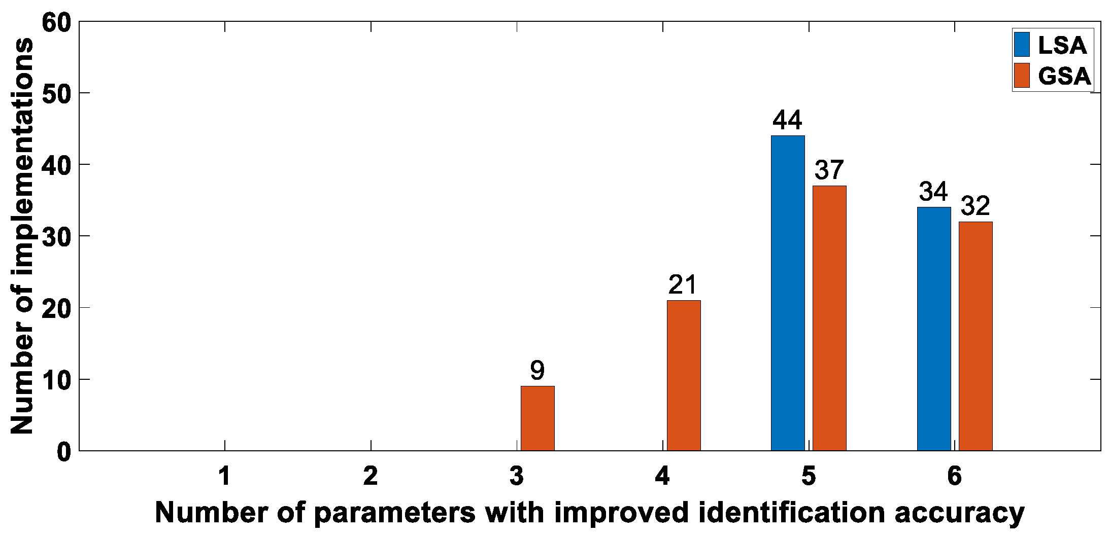
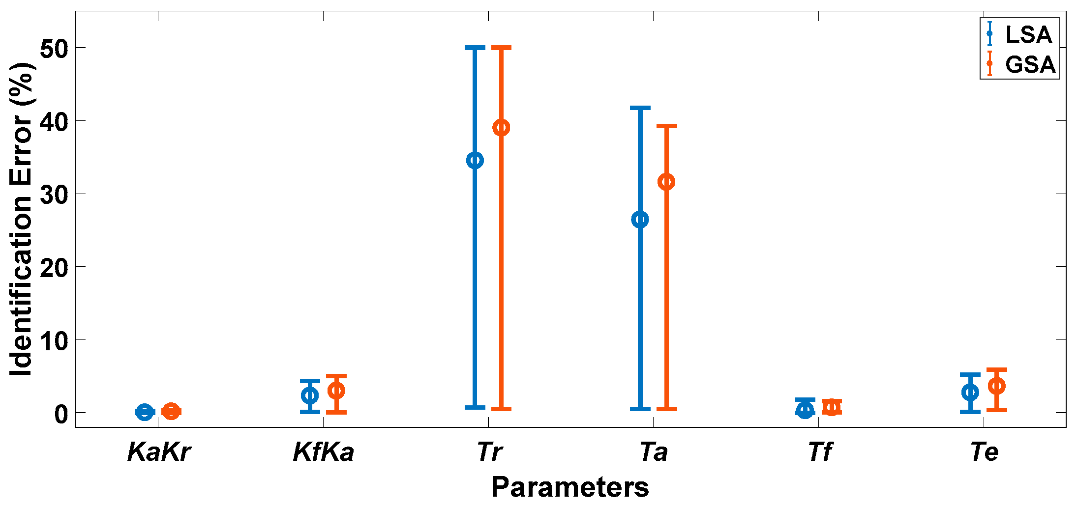
- For parameter groups obtained by LSA, the success rate of GAIS is 78%. In the 100 identifications, the identification accuracy of all parameters was improved in 34 identifications, and the identification accuracy of all key parameters and one non-key parameter was improved in 44 identifications. Table 8 gives an example that only the accuracy of the parameter Tr did not improve, while the identification accuracy of other parameters and the fitting error of the model were significantly improved.
- For parameter groups obtained by GSA, the success rate of GAIS is 99%. In 99 successful identifications, the accuracy of at least three parameters (two key parameters and one non-key parameter) can be improved. The identification accuracy of all parameters is improved in 32 identifications, which is very close to the identification results based on LSA. Table 9 gives an example that the identification accuracy of only the three parameters KaKr, KfKa, and Tf are improved, and the identification accuracy of other parameters remains unchanged or slightly reduced.
7. Conclusions
- The calculation amount of the GSA methods is much larger than that of the LSA method, especially the numerical GSA methods. The GSA method may be inconvenient to use in a model that takes a long time for a single calculation;
- The results of the five GSA methods on the grouping of high- and low-sensitivity parameters are the same. Because the difference in the high- and low-sensitivity values is more prominent in the GSA results, the grouping results of the key and non-key parameters are different from the LSA method;
- Under the strategy of identifying only key parameters, the identification accuracy based on the GSA is not as good as that based on the LSA when the non-key parameters are inaccurate because the GSA enlarges the difference between high- and low-sensitivity values, resulting in more non-key parameters found;
- When the groupwise alternating identification strategy of high- and low-sensitivity parameters is used, the identification accuracy based on the LSA or GSA is equivalent. However, LSA is better than GSA in terms of the corresponding relationship between identification accuracy and sensitivity values.
Author Contributions
Funding
Data Availability Statement
Conflicts of Interest
References
- Ju, P.; Handschin, E. Identifiability of Load Models. IEE Proc. Gener. Transm. Distrib. 1997, 144, 45. [Google Scholar] [CrossRef]
- Choi, B.-K.; Chiang, H.-D. Multiple Solutions and Plateau Phenomenon in Measurement-Based Load Model Development: Issues and Suggestions. IEEE Trans. Power Syst. 2009, 24, 824–831. [Google Scholar] [CrossRef]
- Ju, P.; Jin, Y.; Chen, Q.; Shao, Z.; Mao, C. Identifiability and Identification of a Synthesis Load Model. Sci. China Technol. Sci. 2010, 53, 461–468. [Google Scholar] [CrossRef]
- Qin, C.; Ju, P.; Wu, F.; Liu, L. Distinguishability Analysis of Controller Parameters with Applications to DFIG Based Wind Turbine. Sci. China Technol. Sci. 2013, 56, 2465–2472. [Google Scholar] [CrossRef]
- Moghaddam, I.N.; Salami, Z.; Easter, L. Sensitivity Analysis of an Excitation System in Order to Simplify and Validate Dynamic Model Utilizing Plant Test Data. IEEE Trans. Ind. Appl. 2015, 51, 3435–3441. [Google Scholar] [CrossRef]
- Mitra, P.; Vittal, V. Role of Sensitivity Analysis in Load Model Parameter Estimation. In Proceedings of the 2017 IEEE Power & Energy Society General Meeting, Chicago, IL, USA, 16–20 July 2017; Volume 2018, pp. 1–5. [Google Scholar]
- Ma, J.; Han, D.; He, R.M.; Dong, Z.Y.; Hill, D.J. Reducing Identified Parameters of Measurement-Based Composite Load Model. IEEE Trans. Power Syst. 2008, 23, 76–83. [Google Scholar] [CrossRef]
- Ju, P.; Qin, C.; Wu, F.; Xie, H.; Ning, Y. Load Modeling for Wide Area Power System. Int. J. Electr. Power Energy Syst. 2011, 33, 909–917. [Google Scholar] [CrossRef]
- Son, S.; Lee, S.H.; Choi, D.-H.; Song, K.-B.; Park, J.-D.; Kwon, Y.-H.; Hur, K.; Park, J.-W. Improvement of Composite Load Modeling Based on Parameter Sensitivity and Dependency Analyses. IEEE Trans. Power Syst. 2014, 29, 242–250. [Google Scholar] [CrossRef]
- Zhu, Z.; Geng, G.; Jiang, Q. Multi-Scenario Parameter Estimation for Synchronous Generation Systems. IEEE Trans. Power Syst. 2017, 32, 1851–1859. [Google Scholar] [CrossRef]
- Ghomi, M.; Sarem, Y.N. Review of Synchronous Generator Parameters Estimation and Model Identification. In Proceedings of the 42nd International Universities Power Engineering Conference, Brighton, UK, 4–6 September 2007; pp. 228–235. [Google Scholar] [CrossRef]
- Kian, M.; Najafabadi, T.A.; Lesani, H.; Kazemi, F. Direct Continuous-Time Parameter Identification of Excitation System with the Generator Online. In Proceedings of the 2018 IEEE Texas Power and Energy Conference (TPEC), College Station, TX, USA, 8–9 February 2018; Volume 2018, pp. 1–6. [Google Scholar]
- Saavedra-Montes, A.J.; Ramirez-Scarpetta, J.M.; Ramos-Paja, C.A.; Malik, O.P. Identification of Excitation Systems with the Generator Online. Electr. Power Syst. Res. 2012, 87, 1–9. [Google Scholar] [CrossRef]
- Shi, D.; Tylavsky, D.J.; Koellner, K.M.; Logic, N.; Wheeler, D.E. Transmission Line Parameter Identification Using PMU Measurements. Eur. Trans. Electr. Power 2011, 21, 1574–1588. [Google Scholar] [CrossRef] [Green Version]
- Li, F.; Wang, Q.; Hu, J.X.; Tang, Y. An Estimation and Correction Combined Method for Hvdc Model Parameters Identification. IEEE Access 2021, 9, 51020–51028. [Google Scholar] [CrossRef]
- Arif, A.; Wang, Z.; Wang, J.; Mather, B.; Bashualdo, H.; Zhao, D. Load Modeling—A Review. IEEE Trans. Smart Grid 2018, 9, 5986–5999. [Google Scholar] [CrossRef]
- Abbassi, R.; Abbassi, A.; Jemli, M.; Chebbi, S. Identification of Unknown Parameters of Solar Cell Models: A Comprehensive Overview of Available Approaches. Renew. Sustain. Energy Rev. 2018, 90, 453–474. [Google Scholar] [CrossRef]
- Zhang, J.; Cui, M.; He, Y. Parameters Identification of Equivalent Model of Permanent Magnet Synchronous Generator (PMSG) Wind Farm Based on Analysis of Trajectory Sensitivity. Energies 2020, 13, 4607. [Google Scholar] [CrossRef]
- Hu, Y.-L.; Wu, Y.-K. Review on Model Validation and Parameter Estimation Approaches of Wind Power Generators. J. Eng. 2017, 2017, 2407–2411. [Google Scholar] [CrossRef]
- Guewouo, T.; Luo, L.; Tarlet, D.; Tazerout, M. Identification of Optimal Parameters for a Small-Scale Compressed-Air Energy Storage System Using Real Coded Genetic Algorithm. Energies 2019, 12, 377. [Google Scholar] [CrossRef] [Green Version]
- Borgonovo, E.; Plischke, E. Sensitivity Analysis: A Review of Recent Advances. Eur. J. Oper. Res. 2016, 248, 869–887. [Google Scholar] [CrossRef]
- Douglas-Smith, D.; Iwanaga, T.; Croke, B.F.W.; Jakeman, A.J. Certain Trends in Uncertainty and Sensitivity Analysis: An Overview of Software Tools and Techniques. Environ. Model. Softw. 2020, 124, 104588. [Google Scholar] [CrossRef]
- Ginocchi, M.; Ponci, F.; Monti, A. Sensitivity Analysis and Power Systems: Can We Bridge the Gap? A Review and a Guide to Getting Started. Energies 2021, 14, 8274. [Google Scholar] [CrossRef]
- Song, X.; Zhang, J.; Zhan, C.; Xuan, Y.; Ye, M.; Xu, C. Global Sensitivity Analysis in Hydrological Modeling: Review of Concepts, Methods, Theoretical Framework, and Applications. J. Hydrol. 2015, 523, 739–757. [Google Scholar] [CrossRef] [Green Version]
- Qian, G.; Mahdi, A. Sensitivity Analysis Methods in the Biomedical Sciences. Math. Biosci. 2020, 323, 108306. [Google Scholar] [CrossRef]
- Wagener, T.; Pianosi, F. What Has Global Sensitivity Analysis Ever Done for Us? A Systematic Review to Support Scientific Advancement and to Inform Policy-Making in Earth System Modelling. Earth Sci. Rev. 2019, 194, 1–18. [Google Scholar] [CrossRef]
- Perz, S.G.; Muñoz-Carpena, R.; Kiker, G.; Holt, R.D. Evaluating Ecological Resilience with Global Sensitivity and Uncertainty Analysis. Ecol. Modell. 2013, 263, 174–186. [Google Scholar] [CrossRef]
- Pang, Z.; O’Neill, Z.; Li, Y.; Niu, F. The Role of Sensitivity Analysis in the Building Performance Analysis: A Critical Review. Energy Build. 2020, 209, 109659. [Google Scholar] [CrossRef]
- Saad, S.; Ossart, F.; Bigeon, J.; Sourdille, E.; Gance, H. Global Sensitivity Analysis Applied to Train Traffic Rescheduling: A Comparative Study. Energies 2021, 14, 6420. [Google Scholar] [CrossRef]
- Tsvetkova, O.; Ouarda, T.B.M.J. A Review of Sensitivity Analysis Practices in Wind Resource Assessment. Energy Convers. Manag. 2021, 238, 114112. [Google Scholar] [CrossRef]
- Preece, R.; Milanovic, J.V. Assessing the Applicability of Uncertainty Importance Measures for Power System Studies. IEEE Trans. Power Syst. 2016, 31, 2076–2084. [Google Scholar] [CrossRef]
- Ni, F.; Nijhuis, M.; Nguyen, P.H.; Cobben, J.F.G. Variance-Based Global Sensitivity Analysis for Power Systems. IEEE Trans. Power Syst. 2018, 33, 1670–1682. [Google Scholar] [CrossRef]
- Zhang, B.Z.; Wang, M.; Su, W. Reliability Assessment of Converter- Dominated Power Systems Using Variance-Based Global Sensitivity Analysis. IEEE Open Access J. Power Energy 2021, 8, 248–257. [Google Scholar] [CrossRef]
- Ye, K.; Zhao, J.; Huang, C.; Duan, N.; Zhang, Y.; Field, T. A Data-Driven Global Sensitivity Analysis Framework for Three-Phase Distribution System with PVs. IEEE Trans. Power Syst. 2021, 36, 4809–4819. [Google Scholar] [CrossRef]
- Shuai, C.; Deyou, Y.; Weichun, G.; Chuang, L.; Guowei, C.; Lei, K. Global Sensitivity Analysis of Voltage Stability in the Power System with Correlated Renewable Energy. Electr. Power Syst. Res. 2021, 192, 106916. [Google Scholar] [CrossRef]
- Liao, X.; Zhang, M.; Le, J.; Zhang, L.; Li, Z. Global Sensitivity Analysis of Static Voltage Stability Based on Extended Affine Model. Electr. Power Syst. Res. 2022, 208, 107872. [Google Scholar] [CrossRef]
- Xu, X.; Yan, Z.; Shahidehpour, M.; Wang, H.; Chen, S. Power System Voltage Stability Evaluation Considering Renewable Energy with Correlated Variabilities. IEEE Trans. Power Syst. 2018, 33, 3236–3245. [Google Scholar] [CrossRef]
- Xu, X.; Yan, Z.; Shahidehpour, M.; Chen, S.; Wang, H.; Li, Z.; Zhou, Q. Maximum Loadability of Islanded Microgrids with Renewable Energy Generation. IEEE Trans. Smart Grid 2018, 10, 4696–4705. [Google Scholar] [CrossRef]
- Lu, Z.; Xu, X.; Yan, Z.; Wang, H. Density-Based Global Sensitivity Analysis of Islanded Microgrid Loadability Considering Distributed Energy Resource Integration. J. Mod. Power Syst. Clean Energy 2020, 8, 94–101. [Google Scholar] [CrossRef]
- Hasan, K.N.; Preece, R. Influence of Stochastic Dependence on Small-Disturbance Stability and Ranking Uncertainties. IEEE Trans. Power Syst. 2018, 33, 3227–3235. [Google Scholar] [CrossRef]
- Hasan, K.N.; Preece, R.; Milanovic, J.V. Priority Ranking of Critical Uncertainties Affecting Small-Disturbance Stability Using Sensitivity Analysis Techniques. IEEE Trans. Power Syst. 2017, 32, 2629–2639. [Google Scholar] [CrossRef] [Green Version]
- Cruz May, E.; Bassam, A.; Ricalde, L.J.; Escalante Soberanis, M.A.; Oubram, O.; May Tzuc, O.; Alanis, A.Y.; Livas-García, A. Global Sensitivity Analysis for a Real-Time Electricity Market Forecast by a Machine Learning Approach: A Case Study of Mexico. Int. J. Electr. Power Energy Syst. 2021, 135, 107505. [Google Scholar] [CrossRef]
- Zhang, F.; Wang, X.; Hou, X.; Han, C.; Wu, M.; Liu, Z. Variance-Based Global Sensitivity Analysis of a Hybrid Thermoelectric Generator Fuzzy System. Appl. Energy 2022, 307, 118208. [Google Scholar] [CrossRef]
- Luo, Y.; Wang, Z.; Zhu, J.; Lu, T.; Xiao, G.; Chu, F.; Wang, R. Multi-Objective Robust Optimization of a Solar Power Tower Plant under Uncertainty. Energy 2022, 238, 121716. [Google Scholar] [CrossRef]
- Carta, J.A.; Díaz, S.; Castañeda, A. A Global Sensitivity Analysis Method Applied to Wind Farm Power Output Estimation Models. Appl. Energy 2020, 280, 115968. [Google Scholar] [CrossRef]
- Dong, M.; Li, Y.; Song, D.; Yang, J.; Su, M.; Deng, X.; Huang, L.; Elkholy, M.H.; Joo, Y.H. Uncertainty and Global Sensitivity Analysis of Levelized Cost of Energy in Wind Power Generation. Energy Convers. Manag. 2021, 229, 113781. [Google Scholar] [CrossRef]
- Tian, X.; Lii, X.; Zhao, L.; Tan, Z.; Luo, S.; Li, C. Simplified Identification Strategy of Load Model Based on Global Sensitivity Analysis. IEEE Access 2020, 8, 131545–131552. [Google Scholar] [CrossRef]
- Shen, W.J.; Li, H.X. A Sensitivity-Based Group-Wise Parameter Identification Algorithm for the Electric Model of Li-Ion Battery. IEEE Access 2017, 5, 4377–4387. [Google Scholar] [CrossRef]
- Pianosi, F.; Sarrazin, F.; Wagener, T. A Matlab Toolbox for Global Sensitivity Analysis. Environ. Model. Softw. 2015, 70, 80–85. [Google Scholar] [CrossRef] [Green Version]
- Sarrazin, F.; Pianosi, F.; Wagener, T. An Introduction to the SAFE Matlab Toolbox with Practical Examples and Guidelines. In Sensitivity Analysis in Earth Observation Modelling; Petropoulos, G.P., Srivastava, P.K., Eds.; Elsevier: Amsterdam, The Netherlands, 2017; pp. 363–378. ISBN 978-0-12-803011-0. [Google Scholar]
- Saltelli, A.; Ratto, M.; Andres, T.; Campolongo, F.; Cariboni, J.; Gatelli, D.; Saisana, M.; Tarantola, S. Global Sensitivity Analysis: The Primer; John Wiley & Sons, Ltd.: Chichester, UK, 2007; ISBN 9780470725184. [Google Scholar]
- Lin, Y.; Wang, Y.; Wang, J.; Wang, S.; Shi, D. Global Sensitivity Analysis in Load Modeling via Low-Rank Tensor. IEEE Trans. Smart Grid 2020, 11, 2737–2740. [Google Scholar] [CrossRef] [Green Version]
- Liao, X.; Liu, K.; Le, J.; Zhu, S.; Huai, Q.; Li, B.; Zhang, Y. Extended Affine Arithmetic-Based Global Sensitivity Analysis for Power Flow with Uncertainties. Int. J. Electr. Power Energy Syst. 2020, 115, 105440. [Google Scholar] [CrossRef]
- Han, W.; Yang, P.; Ren, H.; Sun, J. Comparison Study of Several Kinds of Inertia Weights for PSO. In Proceedings of the 2010 IEEE International Conference on Progress in Informatics and Computing, Shanghai, China, 10–12 December 2010; Volume 1, pp. 280–284. [Google Scholar]


| Numerical GSA Method | Visualized GSA Method |
|---|---|
| Sobol method Morris method | Regional sensitivity analysis Scatter plots Andres visualization test |
| Parameter | Symbol | Typical Value |
|---|---|---|
| Filter gain | Kr | 1.00 |
| Regulator gain | Ka | 20.00 |
| Stabilizing circuit gain | Kf | 0.04 |
| Filter time constant | Tr | 0.04 s |
| Regulator time constant | Ta | 0.04 s |
| Stabilizing circuit time constant | Tf | 0.70 s |
| Exciter time constant | Te | 0.80 s |
| Parameter | Value Range | Parameter | Value Range |
|---|---|---|---|
| Kr | [0.01, 2.00] | Tr | [0, 0.06] |
| Ka | [1, 100] | Ta | [0, 0.2] |
| Kf | [0.01, 0.5] | Tf | [0, 2] |
| Te | [0, 2] |
| Method | Amount of Calculation | Method | Amount of Calculation |
|---|---|---|---|
| LSA | 2 × N | RSA | Ns |
| Sobol | (N + 2) × Ns | Scatter plot | Ns |
| Morris | (N + 1) × Ns | AVT | Ns |
| Result | Parameters | Fitting Error | |||||
|---|---|---|---|---|---|---|---|
| * Tr | * Ta | KaKr | KfKa | Tf | Te | ||
| 1 | 0.049 | 0.181 | 18.54 | 1.018 | 0.472 | 0.546 | 0.29% |
| 2 | 0.060 | 0.077 | 19.46 | 0.887 | 0.626 | 0.693 | 0.16% |
| 3 | 0.056 | 0.083 | 19.44 | 0.890 | 0.620 | 0.688 | 0.16% |
| 4 | 0.047 | 0.112 | 19.26 | 0.938 | 0.579 | 0.629 | 0.20% |
| 5 | 0.018 | 0.106 | 19.72 | 0.865 | 0.626 | 0.704 | 0.11% |
| 6 | 0.056 | 0.044 | 19.86 | 0.837 | 0.680 | 0.754 | 0.05% |
| 7 | 0.032 | 0.086 | 19.71 | 0.845 | 0.645 | 0.735 | 0.11% |
| 8 | 0.017 | 0.050 | 20.26 | 0.784 | 0.712 | 0.809 | 0.04% |
| 9 | 0.050 | 0.030 | 19.90 | 0.815 | 0.766 | 0.846 | 0.07% |
| 10 | 0.015 | 0.075 | 20.00 | 0.799 | 0.682 | 0.789 | 0.03% |
| Emin | — | — | 0.02% | 0.11% | 1.78% | 1.13% | 0.03% |
| Emax | — | — | 7.30% | 27.3% | 32.6% | 31.8% | 0.29% |
| Eavr | — | — | 2.19% | 8.90% | 10.7% | 11.5% | 0.12% |
| Result | Parameters | Fitting Error | |||||
|---|---|---|---|---|---|---|---|
| * Tr | * Ta | * Tf | * Te | KaKr | KfKa | ||
| 1 | 0.053 | 0.200 | 1.599 | 1.558 | 16.04 | 0.369 | 0.77% |
| 2 | 0.032 | 0.036 | 0.461 | 1.995 | 15.58 | 0.078 | 0.69% |
| 3 | 0.035 | 0.116 | 0.045 | 0.548 | 16.73 | 1.198 | 0.59% |
| 4 | 0.011 | 0.169 | 1.571 | 1.191 | 18.25 | 0.648 | 0.63% |
| 5 | 0.048 | 0.003 | 0.953 | 1.625 | 17.20 | 0.262 | 0.46% |
| 6 | 0.021 | 0.065 | 1.315 | 0.649 | 18.90 | 0.984 | 0.55% |
| 7 | 0.022 | 0.043 | 0.475 | 1.002 | 18.99 | 0.668 | 0.27% |
| 8 | 0.042 | 0.159 | 1.534 | 1.503 | 16.75 | 0.408 | 0.68% |
| 9 | 0.051 | 0.170 | 0.539 | 1.301 | 16.26 | 0.501 | 0.55% |
| 10 | 0.027 | 0.123 | 1.157 | 0.669 | 20.07 | 0.950 | 0.51% |
| Emin | — | — | — | — | 0.36% | 16.5% | 0.27% |
| Emax | — | — | — | — | 22.1% | 90.3% | 0.77% |
| Eavr | — | — | — | — | 12.7% | 42.5% | 0.57% |
| Result | Parameters | Fitting Error | ||||
|---|---|---|---|---|---|---|
| Kr | Ka | Kf | KaKr | KfKa | ||
| 1 | 0.678 | 27.35 | 0.037 | 18.54 | 1.018 | 0.29% |
| 2 | 1.457 | 13.36 | 0.066 | 19.46 | 0.887 | 0.16% |
| 3 | 0.218 | 89.00 | 0.010 | 19.44 | 0.890 | 0.16% |
| 4 | 0.911 | 21.15 | 0.044 | 19.26 | 0.938 | 0.20% |
| 5 | 1.187 | 16.61 | 0.052 | 19.72 | 0.865 | 0.11% |
| 6 | 0.764 | 26.00 | 0.032 | 19.86 | 0.837 | 0.05% |
| 7 | 1.582 | 12.45 | 0.068 | 19.71 | 0.845 | 0.11% |
| 8 | 0.258 | 78.38 | 0.010 | 20.26 | 0.784 | 0.04% |
| 9 | 0.344 | 57.89 | 0.014 | 19.90 | 0.815 | 0.07% |
| 10 | 0.250 | 79.91 | 0.010 | 20.00 | 0.799 | 0.03% |
| Emin | 8.92% | 5.73% | 6.94% | 0.02% | 0.11% | 0.03% |
| Emax | 78.2% | 344% | 75.0% | 7.30% | 27.3% | 0.29% |
| Eavr | 48.0% | 128% | 49.3% | 2.19% | 8.90% | 0.12% |
| Result | Parameters | Fitting Error | |||||
|---|---|---|---|---|---|---|---|
| KaKr | KfKa | Tr | Ta | Tf | Te | ||
| Initial | 18.95 | 0.871 | 0.034 | 0.137 | 0.457 | 0.688 | 0.25% |
| 5.26% | 8.88% | 14.4% | 242% | 34.7% | 14.0% | ||
| Final | 19.99 | 0.812 | 0.052 | 0.032 | 0.687 | 0.778 | 0.01% |
| 0.07% | 1.45% | 28.7% | 20.5% | 1.81% | 2.72% | ||
| Result | Parameters | Fitting Error | |||||
|---|---|---|---|---|---|---|---|
| KaKr | KfKa | Tr | Ta | Tf | Te | ||
| Initial | 20.42 | 0.893 | 0.031 | 0.052 | 0.800 | 0.812 | 0.11% |
| 2.09% | 11.6% | 23.8% | 30.0% | 14.3% | 1.49% | ||
| Final | 20.03 | 0.826 | 0.057 | 0.028 | 0.701 | 0.767 | 0.01% |
| 0.16% | 3.19% | 42.6% | 30.3% | 0.12% | 4.09% | ||
Disclaimer/Publisher’s Note: The statements, opinions and data contained in all publications are solely those of the individual author(s) and contributor(s) and not of MDPI and/or the editor(s). MDPI and/or the editor(s) disclaim responsibility for any injury to people or property resulting from any ideas, methods, instructions or products referred to in the content. |
© 2023 by the authors. Licensee MDPI, Basel, Switzerland. This article is an open access article distributed under the terms and conditions of the Creative Commons Attribution (CC BY) license (https://creativecommons.org/licenses/by/4.0/).
Share and Cite
Qin, C.; Jin, Y.; Tian, M.; Ju, P.; Zhou, S. Comparative Study of Global Sensitivity Analysis and Local Sensitivity Analysis in Power System Parameter Identification. Energies 2023, 16, 5915. https://doi.org/10.3390/en16165915
Qin C, Jin Y, Tian M, Ju P, Zhou S. Comparative Study of Global Sensitivity Analysis and Local Sensitivity Analysis in Power System Parameter Identification. Energies. 2023; 16(16):5915. https://doi.org/10.3390/en16165915
Chicago/Turabian StyleQin, Chuan, Yuqing Jin, Meng Tian, Ping Ju, and Shun Zhou. 2023. "Comparative Study of Global Sensitivity Analysis and Local Sensitivity Analysis in Power System Parameter Identification" Energies 16, no. 16: 5915. https://doi.org/10.3390/en16165915
APA StyleQin, C., Jin, Y., Tian, M., Ju, P., & Zhou, S. (2023). Comparative Study of Global Sensitivity Analysis and Local Sensitivity Analysis in Power System Parameter Identification. Energies, 16(16), 5915. https://doi.org/10.3390/en16165915