
Open-Access Model of a PV–BESS System: Quantifying Power and Energy Exchange for Peak-Shaving and Self Consumption Applications

 , , and
Abstract
1. Introduction
1.1. Relevant Literature
1.2. Contributions
- Describing in detail two open-access models for PV systems that can be coupled with a BESS model, detailing how all the parts integrate into a general PV–BESS model;
- Proposing the most suitable uses for each PV system model, based on their inherent advantages and drawbacks and available data;
- Making available a model for two different modes of operation, i.e., a PV–BESS for peak-shaving applications and a PV–BESS system that maximizes self-consumption; and
- Demonstrating the dynamics of a PV–BESS system using both integrated models for peak-shaving and self-consumption applications, validating them with measurements of a PV system in Costa Rica.
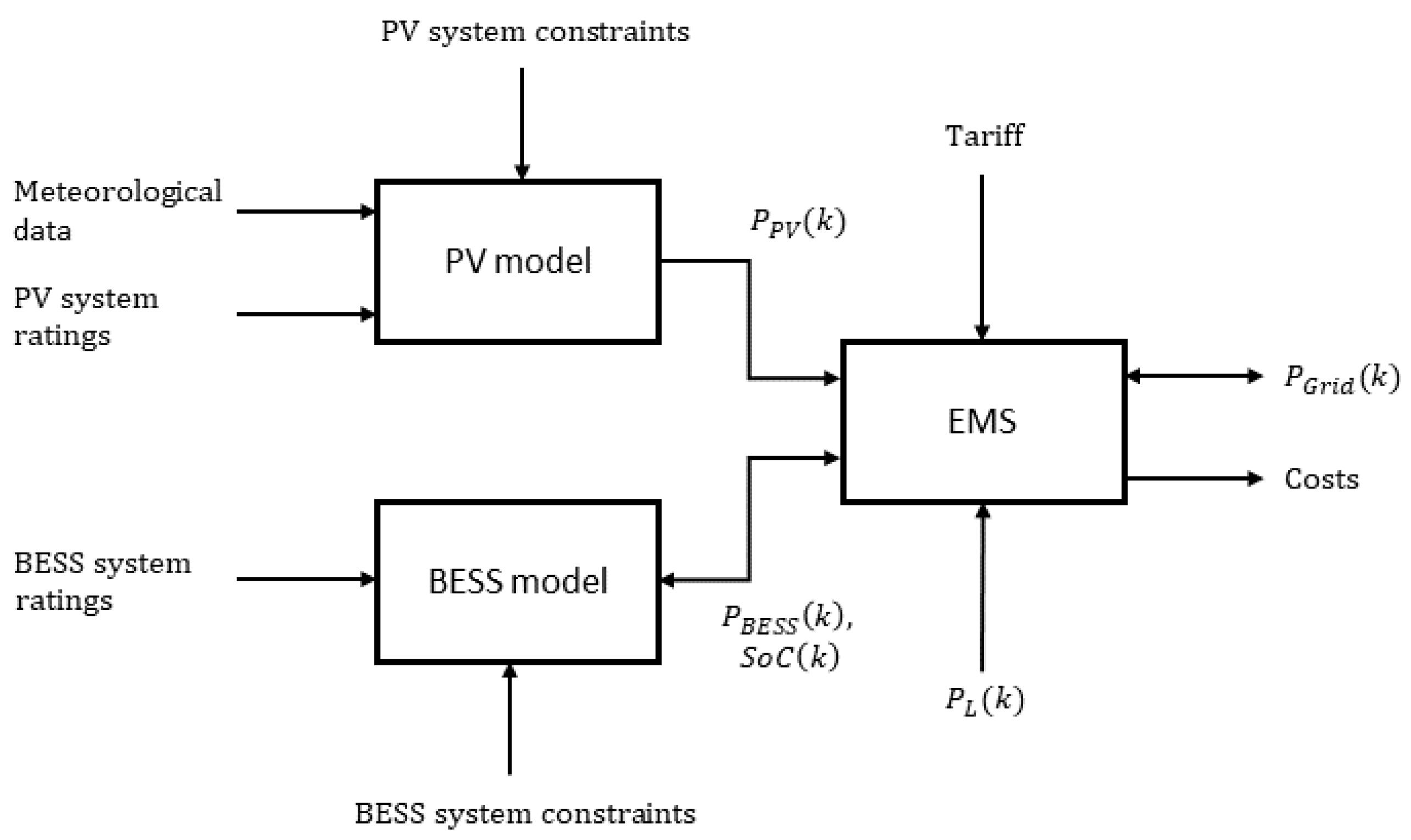
2. PV–BESS Model
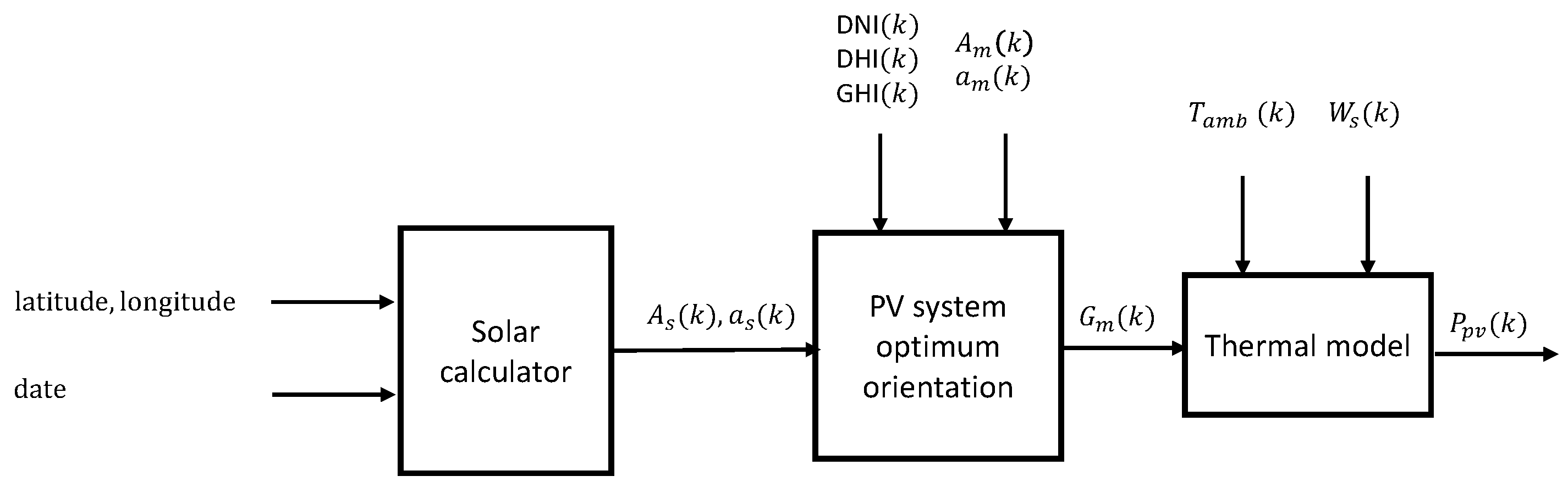
2.1. PV Modeling
2.1.1. Meteorological Data-Based Model
2.1.2. Gaussian Model
2.1.3. Battery Modeling
3. Inputs to the Models
3.1. PV System Installed
3.2. Load
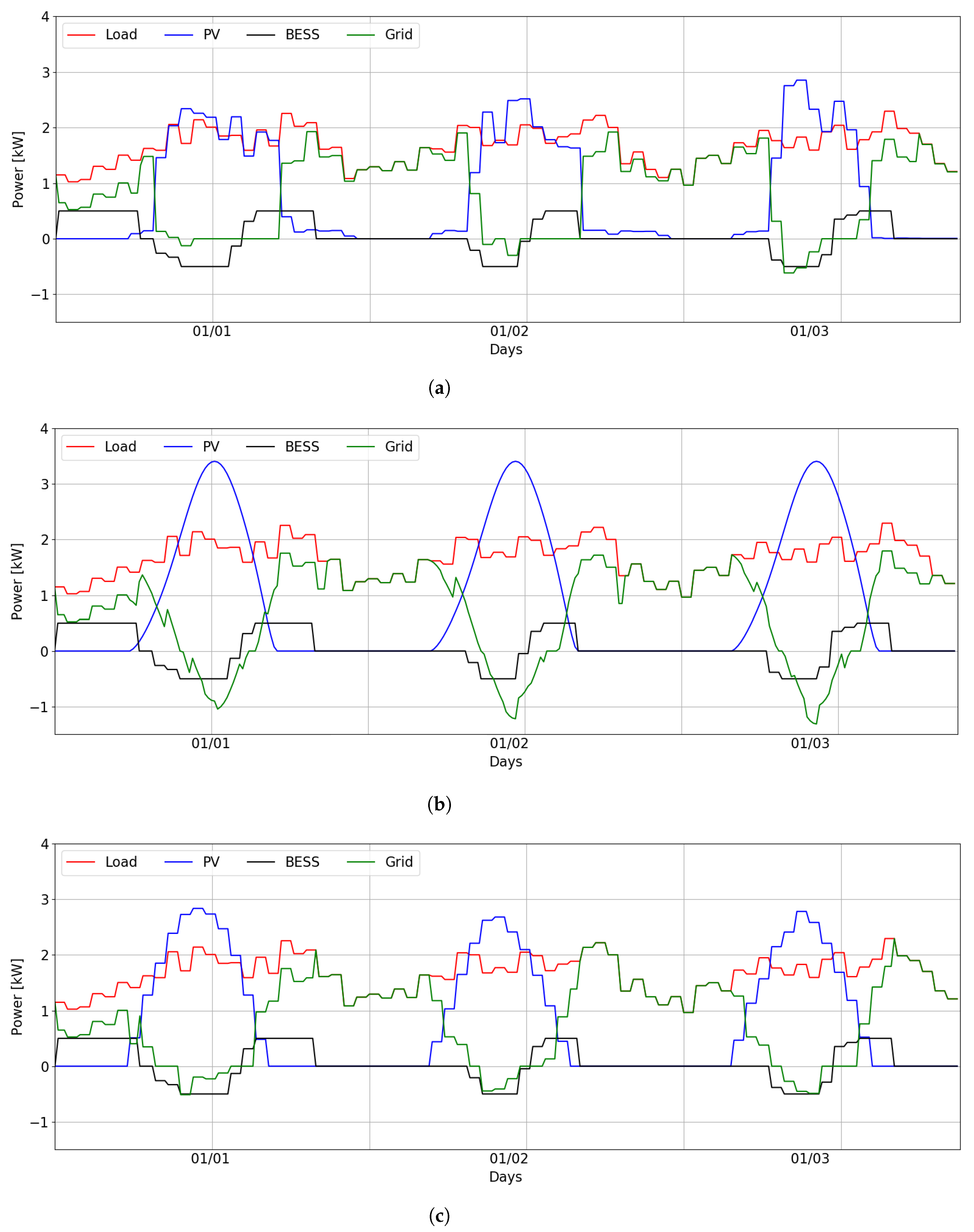
4. Results and Discussion
4.1. PV Generation
4.2. PV–BESS
4.2.1. Self-Consumption
4.2.2. Peak-Shaving
5. Conclusions
Author Contributions
Funding
Data Availability Statement
Acknowledgments
Conflicts of Interest
Abbreviations
| BESS | Battery Energy Storage System |
| DG | Distributed Generation |
| DR | Demand Response |
| DSO | Distribution System Operators |
| EMS | Energy Management Systems |
| ESS | Energy Storage Systems |
| RES | Renewable Energy Sources |
| SoC | State-of-Charge |
References
- IRENA. World Energy Transitions Outlook: 1.5 °C Pathway; IRENA: Masdar City, United Arab Emirates, 2021; pp. 1–312. [Google Scholar]
- Alpízar-Castillo, J.; Ramírez-Elizondo, L.; Bauer, P. The Effect of Non-Coordinated Heating Electrification Alternatives on a Low-Voltage Distribution Network with High PV Penetration. In Proceedings of the 2023 IEEE 17th International Conference on Compatibility, Power Electronics, and Power Engineering (CPE-POWERENG), Tallinn, Estonia, 14–16 June 2023. [Google Scholar]
- Alpízar-Castillo, J.; Ramirez-Elizondo, L.; Bauer, P. Assessing the Role of Energy Storage in Multiple Energy Carriers toward Providing Ancillary Services: A Review. Energies 2023, 16, 379. [Google Scholar] [CrossRef]
- IRENA. Renewable Power Generation Costs in 2021; IRENA: Masdar City, United Arab Emirates, 2022. [Google Scholar]
- Alotaibi, I.; Abido, M.A.; Khalid, M.; Savkin, A.V. A comprehensive review of recent advances in smart grids: A sustainable future with renewable energy resources. Energies 2020, 13, 6269. [Google Scholar] [CrossRef]
- Van Sark, W. Photovoltaic System Design and Performance. Energies 2019, 12, 1826. [Google Scholar] [CrossRef]
- PVsyst–Logiciel Photovoltaïque. 2023. Available online: https://www.pvsyst.com/fr/ (accessed on 17 February 2023).
- PV*SOL–Plan and Design Better pv Systems with Professional Solar Software|PV*SOL and PV*SOL Premium. 2023. Available online: https://pvsol.software/en/ (accessed on 17 February 2023).
- Sanjari, M.J.; Gooi, H.B. Probabilistic Forecast of PV Power Generation Based on Higher Order Markov Chain. IEEE Trans. Power Syst. 2017, 32, 2942–2952. [Google Scholar] [CrossRef]
- Carriere, T.; Vernay, C.; Pitaval, S.; Kariniotakis, G. A Novel Approach for Seamless Probabilistic Photovoltaic Power Forecasting Covering Multiple Time Frames. IEEE Trans. Smart Grid 2020, 11, 2281–2292. [Google Scholar] [CrossRef]
- Bessa, R.J.; Trindade, A.; Silva, C.S.; Miranda, V. Probabilistic solar power forecasting in smart grids using distributed information. Int. J. Electr. Power Energy Syst. 2015, 72, 16–23. [Google Scholar] [CrossRef]
- Li, G.; Guo, S.; Li, X.; Cheng, C. Short-term Forecasting Approach Based on bidirectional long short-term memory and convolutional neural network for Regional Photovoltaic Power Plants. Sustain. Energy Grids Netw. 2023, 34, 101019. [Google Scholar] [CrossRef]
- Rana, M.M.; Romlie, M.F.; Abdullah, M.F.; Uddin, M.; Sarkar, M.R. A novel peak load shaving algorithm for isolated microgrid using hybrid PV-BESS system. Energy 2021, 234, 1157. [Google Scholar] [CrossRef]
- Rezaul Alam, M.; Alam, M.; Saha, T.K.; Sohrab Hasan Nizami, M. A PV variability tolerant generic multifunctional control strategy for battery energy storage systems in solar PV plants. Int. J. Electr. Power Energy Syst. 2023, 153, 109315. [Google Scholar] [CrossRef]
- Singh, R.; Bansal, R.; Singh, A.R. Optimization of an isolated photo-voltaic generating unit with battery energy storage system using electric system cascade analysis. Electr. Power Syst. Res. 2018, 164, 188–200. [Google Scholar] [CrossRef]
- Duman, A.C.; Erden, H.S.; Gönül, Ö.; Güler, Ö. Optimal sizing of PV-BESS units for home energy management system-equipped households considering day-ahead load scheduling for demand response and self-consumption. Energy Build. 2022, 267, 112164. [Google Scholar] [CrossRef]
- Hassan, M.U.; Saha, S.; Haque, M.E. A framework for the performance evaluation of household rooftop solar battery systems. Int. J. Electr. Power Energy Syst. 2021, 125, 106446. [Google Scholar] [CrossRef]
- Kim, I.; James, J.A.; Crittenden, J. The case study of combined cooling heat and power and photovoltaic systems for building customers using HOMER software. Electr. Power Syst. Res. 2017, 143, 490–502. [Google Scholar] [CrossRef]
- Li, Q.; Tao, Y.; Li, Z.; Zhang, Y.; Zhang, Z. Simulation and modeling for active distribution network BESS system in DIgSILENT. Energy Rep. 2022, 8, 97–102. [Google Scholar] [CrossRef]
- ERA-Interim. Climate Data Guide; National Center for Atmospheric Research: Boulder, CO, USA, 2018. [Google Scholar]
- Narayan, N.; Papakosta, T.; Vega-Garita, V.; Qin, Z.; Popovic-Gerber, J.; Bauer, P.; Zeman, M. Estimating battery lifetimes in Solar Home System design using a practical modelling methodology. Appl. Energy 2018, 228, 1629–1639. [Google Scholar] [CrossRef]
- Vega-Garita, V.; Hanif, A.; Narayan, N.; Ramirez-Elizondo, L.; Bauer, P. Selecting a suitable battery technology for the photovoltaic battery integrated module. J. Power Sources 2019, 438, 227011. [Google Scholar] [CrossRef]
- Narayan, N.; Vega-Garita, V.; Qin, Z.; Popovic-Gerber, J.; Bauer, P.; Zeman, M. A modeling methodology to evaluate the impact of temperature on Solar Home Systems for rural electrification. In Proceedings of the 2018 IEEE International Energy Conference, ENERGYCON 2018, Limassol, Cyprus, 3–7 June 2018. [Google Scholar] [CrossRef]
- Vega-Garita, V.; De Lucia, D.; Narayan, N.; Ramirez-Elizondo, L.; Bauer, P. PV-battery integrated module as a solution for off-grid applications in the developing world. In Proceedings of the 2018 IEEE International Energy Conference, ENERGYCON 2018, Limassol, Cyprus, 3–7 June 2018. [Google Scholar] [CrossRef]
- Alpízar-Castillo, J.; Vega-Garita, V. PV BESS Model. 2023. Available online: https://github.com/jjac13/PV_BESS_model (accessed on 6 June 2023).
- US Naval Observatory Astronomical Applications Department. Computing Approximate Solar Coordinates. 2023. Available online: https://aa.usno.navy.mil/faq/sun_approx (accessed on 17 February 2023).
- Duffie, J.A.; Beckman, W.A. Solar Engineering of Thermal Processes; Wiley: Hoboken, NJ, USA, 2013; p. 936. [Google Scholar]
- Alpízar-Castillo, J. Simplified Model to Approach the Theoretical Clear Sky Solar PV Generation Curve through a Gaussian Approximation. Niger. J. Technol. 2021, 40, 44–48. [Google Scholar] [CrossRef]
- Wang, L.; Yan, R.; Saha, T.K. Voltage regulation challenges with unbalanced PV integration in low voltage distribution systems and the corresponding solution. Appl. Energy 2019, 256, 113927. [Google Scholar] [CrossRef]
- Datta, U.; Kalam, A.; Shi, J. Smart control of BESS in PV integrated EV charging station for reducing transformer overloading and providing battery-to-grid service. J. Energy Storage 2020, 28, 113927. [Google Scholar] [CrossRef]
- Stecca, M.; Elizondo, L.R.; Soeiro, T.B.; Bauer, P.; Palensky, P. A comprehensive review of the integration of battery energy storage systems into distribution networks. IEEE Open J. Ind. Electron. Soc. 2020, 1, 46–65. [Google Scholar] [CrossRef]
- ICE. Plan de Expansión de la Generación Eléctrica 2018–2034; Technical Report; ICE: London, UK, 2019. [Google Scholar]


| BESS Model | PV Model | Control | Requirements | Language | Ref. |
|---|---|---|---|---|---|
| Simulink© block | Simulink© block | Rule-based | Irradiance, temperature, PV system rating, BESS rating | Matlab-Simulink© | [13] |
| Energy balance | - | Multifunctional control | PV generation data, BESS rating | Matlab©, RSCAD-RTDS© | [14] |
| Energy balance | Analytical approximation | Electric system cascade analysis (ESCA) (rule-based) | Irradiance, temperature, sun altitude, latitude, | Matlab© | [15] |
| Energy balance | Isotropic solar radiation | Mixed-integer linear programming (MILP) | Irradiance, temperature, latitude, PV system rating, BESS rating | Matlab© | [16] |
| Energy balance | - | Monte-Carlo | PV generation data, BESS rating | Not indicated | [17] |
| Proprietary software | Proprietary software | Proprietary software | Irradiance, latitude and longitude, PV system rating, BESS rating | HOMER© | [18] |
| Voltage source in series with an internal resistor | - | PQ control | PV generation data, BESS rating | DIgSILENT© | [19] |
| Period | Timeframe | Cost ($/kWh) |
|---|---|---|
| Night | 00:01–06:00 | 0.04646 |
| 20:01–00:00 | ||
| Valley | 06:01–10:00 | 0.11102 |
| 12:31–17:30 | ||
| Peak | 10:01–12:30 | 0.27079 |
| 17:30–20:00 |
| Parameter | Symbol | Value | Unit |
|---|---|---|---|
| BESS | |||
| Energy | 10.78 | kWh | |
| Power of the converter | 0.5 | kW | |
| Charging efficiency | 97 | % | |
| Discharging efficiency | 97 | % | |
| Initial state-of-charge | SoC | 50 | % |
| Minimum state-of-charge | SoC | 20 | % |
| Maximum state-of-charge | SoC | 80 | % |
| PV system | |||
| Peak power | 5.525 | kW | |
| Power of the inverter | 7.6 | kW | |
| Tilt of the modules | 10.5 | ° | |
| Azimuth of the modules | 200 | ° | |
| Albedo coefficient | 0.2 | ||
| Module efficiency at STC | 16.19 | % | |
| Thermal coefficient | −0.0035 | ||
| Month | Measurements | Gauss Model | MDB Model |
|---|---|---|---|
| ($) | ($) | ($) | |
| January | 75.36 | 53.29 | 47.70 |
| February | 47.63 | 45.02 | 40.24 |
| March | 27.31 | 49.66 | 48.68 |
| April | 44.98 | 63.52 | 48.01 |
| May | 83.08 | 74.59 | 55.72 |
| June | 83.69 | 74.44 | 66.90 |
| July | 84.48 | 80.29 | 64.87 |
| August | 76.90 | 76.49 | 65.02 |
| September | 62.45 | 71.46 | 57.17 |
| October | 77.60 | 79.52 | 70.55 |
| November | 79.77 | 74.98 | 60.49 |
| December | 87.74 | 63.69 | 60.28 |
| Total | 830.98 | 806.95 | 685.64 |
Disclaimer/Publisher’s Note: The statements, opinions and data contained in all publications are solely those of the individual author(s) and contributor(s) and not of MDPI and/or the editor(s). MDPI and/or the editor(s) disclaim responsibility for any injury to people or property resulting from any ideas, methods, instructions or products referred to in the content. |
© 2023 by the authors. Licensee MDPI, Basel, Switzerland. This article is an open access article distributed under the terms and conditions of the Creative Commons Attribution (CC BY) license (https://creativecommons.org/licenses/by/4.0/).
Share and Cite
Alpízar-Castillo, J.; Vega-Garita, V.; Narayan, N.; Ramirez-Elizondo, L. Open-Access Model of a PV–BESS System: Quantifying Power and Energy Exchange for Peak-Shaving and Self Consumption Applications. Energies 2023, 16, 5480. https://doi.org/10.3390/en16145480
Alpízar-Castillo J, Vega-Garita V, Narayan N, Ramirez-Elizondo L. Open-Access Model of a PV–BESS System: Quantifying Power and Energy Exchange for Peak-Shaving and Self Consumption Applications. Energies. 2023; 16(14):5480. https://doi.org/10.3390/en16145480
Chicago/Turabian StyleAlpízar-Castillo, Joel, Victor Vega-Garita, Nishant Narayan, and Laura Ramirez-Elizondo. 2023. "Open-Access Model of a PV–BESS System: Quantifying Power and Energy Exchange for Peak-Shaving and Self Consumption Applications" Energies 16, no. 14: 5480. https://doi.org/10.3390/en16145480
APA StyleAlpízar-Castillo, J., Vega-Garita, V., Narayan, N., & Ramirez-Elizondo, L. (2023). Open-Access Model of a PV–BESS System: Quantifying Power and Energy Exchange for Peak-Shaving and Self Consumption Applications. Energies, 16(14), 5480. https://doi.org/10.3390/en16145480