Article

Short-Term Wind Power Prediction Based on CEEMDAN-SE and Bidirectional LSTM Neural Network with Markov Chain

1
Hubei Collaborative Innovation Center for High-Efficiency Utilization of Solar Energy, Hubei University of Technology, Wuhan 430068, China
2
Yichang Power Supply Company, State Grid Hubei Electric Power Co., Ltd., Yichang 443200, China
*
Author to whom correspondence should be addressed.
Energies 2023, 16(14), 5476; https://doi.org/10.3390/en16145476
Submission received: 29 June 2023 / Revised: 14 July 2023 / Accepted: 17 July 2023 / Published: 19 July 2023
(This article belongs to the Special Issue Modern Power System Stability and Optimal Operating)

Abstract

:
Accurate wind power data prediction is crucial to increase wind energy usage since wind power data are characterized by uncertainty and randomness, which present significant obstacles to the scheduling of power grids. This paper proposes a hybrid model for wind power prediction based on complementary ensemble empirical mode decomposition with adaptive noise (CEEMDAN), sample entropy (SE), bidirectional long short-term memory network (BiLSTM), and Markov chain (MC). First, CEEMDAN is used to decompose the wind power series into a series of subsequences at various frequencies, and then SE is employed to reconstruct the wind power series subsequences to reduce the model’s complexity. Second, the long short-term memory (LSTM) network is optimized, the BiLSTM neural network prediction method is used to predict each reconstruction component, and the results of the different component predictions are superimposed to acquire the total prediction results. Finally, MC is used to correct the model’s total prediction results to increase the accuracy of the predictions. Experimental validation with measured data from wind farms in a region of Xinjiang, and computational results demonstrate that the proposed model can better fit wind power data than other prediction models and has greater prediction accuracy and generalizability for enhancing wind power prediction performance.

1. Introduction

Intending to achieve zero carbon emissions in all countries, the global generation and installed capacity of new energy are gradually increasing, and the sector is entering a period of rapid development [1]. As a clean energy source, wind power contributes to the goal of zero carbon emissions [2]. The Global Wind Energy Council (GWEC) released the Global Wind Report 2023 [3], which indicates that 77.6 GW of wind power was installed globally in 2022, with a cumulative installed capacity of 906 GW, an increase of 8.3% over the previous year. With the increasing global demand for net-zero greenhouse gas emissions and the pressing need to attain energy security, the market outlook for the global wind power industry is expected to become even more optimistic. However, due to the high uncertainty and randomness of wind power, the grid must reserve a substantial quantity of spare capacity to mitigate the effects of this uncertainty and randomness [4]. Therefore, improving the accuracy of wind power prediction can help promote new energy consumption to effectively manage and dispatch wind power generation systems.
There are three primary methods for forecasting wind power. The first is a physical method, which requires the use of a range of geographical information. Wind power is obtained by incorporating wind power data into the numerical weather prediction (NWP) model and combining it with geographic information surrounding the wind turbine. Globally, several wind energy forecasting systems based on physical methodologies and applicable to global or local regions have been developed. The Wind Atlas Analysis and Application Program (WAsP) model, which was created by Ris National Laboratory in Denmark [5], has been widely utilized in wind energy resource assessment and forecasting throughout the globe. In Ref. [6], applying numerical weather forecasting to the field of wind power prediction, the k-means clustering algorithm is used to process NWP data, simplify the prediction model, and increase the accuracy of the prediction. Ref. [7] combines sequential forward feature selection algorithms and NWP models for power prediction to improve the overall quality of wind power forecasting. The second method is the statistical method, which predicts future wind power by establishing the relationship between historical data and wind power. The methods used are the autoregressive (AR) [8] model, the autoregressive moving average (ARMA) [9] model, the autoregressive integrated moving average (ARIMA) [10] model, and the generalized autoregressive conditional heteroskedasticity (GRACH) [11] model. These models predict future data with the linear characteristics of historical data. Due to the volatility of wind power, these algorithms are ineffective at predicting nonlinear wind power data. With the accelerated development of deep learning, numerous deep-learning models, such as convolutional neural networks (CNNs) [12], support vector machines (SVMs) [13], and LSTM [14], are utilized in the field of wind power prediction. Ref. [15] proposed an ultra-short-term prediction method for wind farm power generation based on long- and short-term memory networks, which has a higher prediction accuracy than artificial neural networks and support vector machines. However, using a single AI method for long-time series training can fall into the problem of local optimum or overfitting, bringing errors into the prediction results.
The third strategy involves combining prediction models. A single prediction model cannot attain a higher level of prediction accuracy; however, combining multiple models can improve prediction performance. Based on the various possible combinations, they can be broadly categorized as data correction prediction models and multi-step processing prediction models. Considering the issue of bias in the prediction results, [16] proposes an NWP wind speed correction model, and the corrected NWP wind speed is utilized for wind power prediction. In Ref. [17], combining optical gradient augmentation machine (LigutGBM) and BiLSTM for prediction, the LigutGBM method is used to correct the prediction error of the neural network model, and the results demonstrate that LigutGBM can further improve the prediction accuracy compared to the original method.
Considering that the fluctuations of wind power data cannot be accurately described by a single model, many researchers have adopted a multi-step processing approach to make predictions to extract the complete characteristics of wind power data in recent years. Initially, the original wind power sequence is decomposed, then the sequence is initially processed, the decomposed subsequence is predicted by a neural network model, and then the predicted data are superimposed to obtain the final predicted value [18]. Ref. [19] introduces singular entropy to evaluate and eliminate data following singular spectrum decomposition and then contrasts and calculates various preprocessing methods using artificial neural network models. Ref. [20] uses variational modal decomposition to decompose the original data into multiple eigenmodal functions, then uses the Max-Relevance and Min-Redundancy algorithm to analyze the correlation between the modes, and then predicts them using the improved LSTM algorithm, achieving good results.
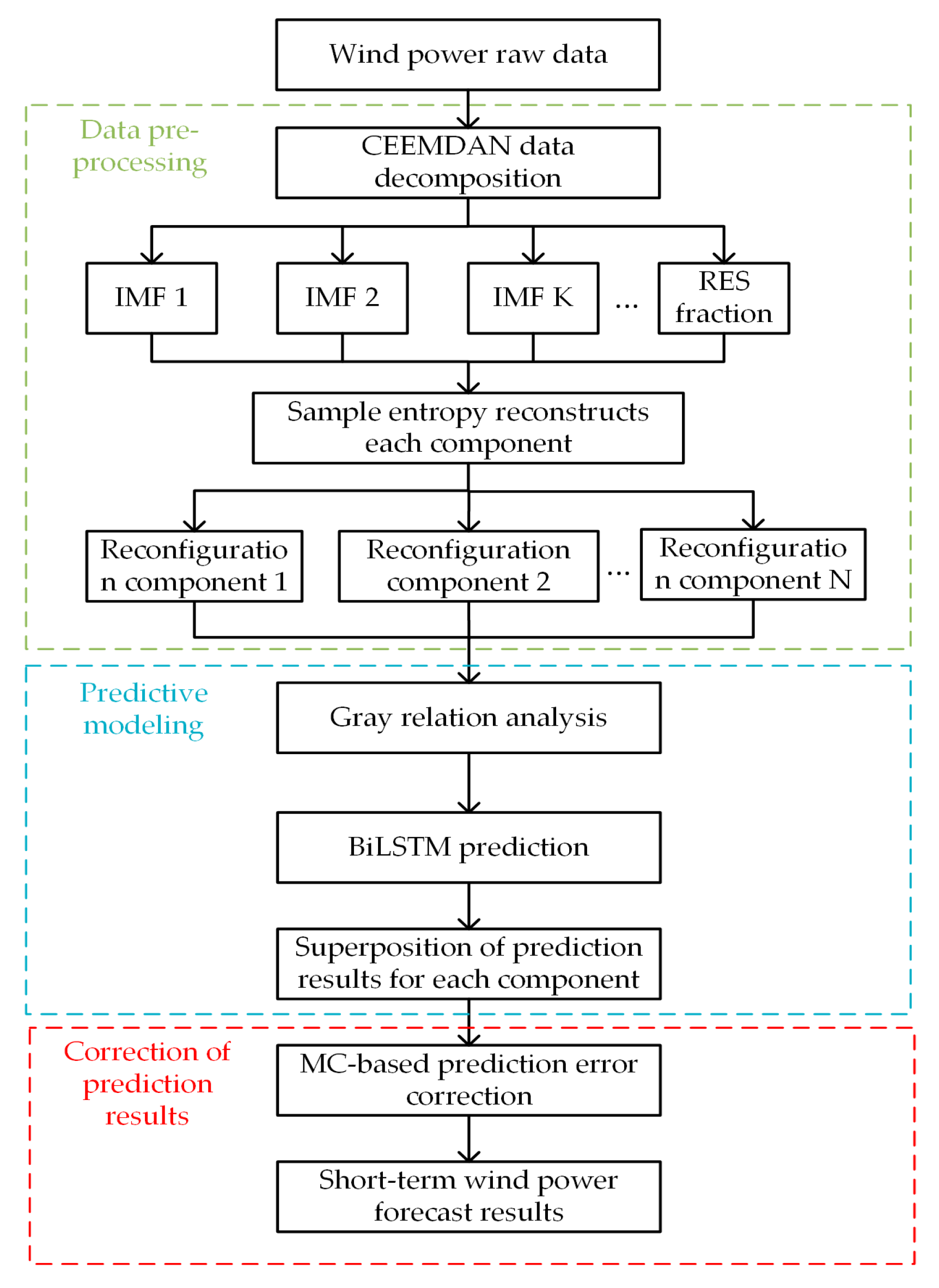
Based on the above analysis, this paper combines data correction and multi-step prediction to propose a wind power prediction model based on improved CEEMDAN and Markov chain. Initially, the original wind power data are preprocessed by CEEMDAN to obtain multiple intrinsic mode function (IMF) components and residual components; secondly, the components are reconstructed by using sample entropy and combined into several different new components based on the entropy value; subsequently, the different components are predicted by using BiLSTM neural network, and the data are superimposed to obtain the total predicted value; finally, the predicted values are data-corrected following the original wind power data.
Experiments on a wind power data set from a region in Xinjiang validate the model’s ability to improve prediction accuracy and prediction efficiency relative to other models. The following are the primary contributions of this paper.
  • A hybrid prediction model that incorporates CEEMDAN, SE, BiLSTM, and MC is proposed. In comparison to EMD, CEEMDAN is capable of resolving the issues of modal mixing and incomplete decomposition, as well as enhancing the efficacy of decomposition.
  • The decomposed subsequences are reconstructed by using SE to combine components with close entropy values into one reconstructed component to eliminate redundant features of wind power data, improve prediction accuracy and shorten prediction time.
  • An improved LSTM neural network model, BiLSTM neural network, is utilized. BiLSTM is a network with two LSTMs in reverse parallel, which can transmit both forward and reverse information to better mine the wind power data information.
  • MC is used to correct the data after the neural network prediction, and the k-step transfer matrix is used to characterize the data deviation, bringing the corrected data closer to the actual value.
  • The model of this paper was compared to other prediction models, validated on the data set, and evaluated by four indicators to demonstrate its superiority over other models.

2. Wind Power Data Pre-Processing

2.1. Wind Power Data Source

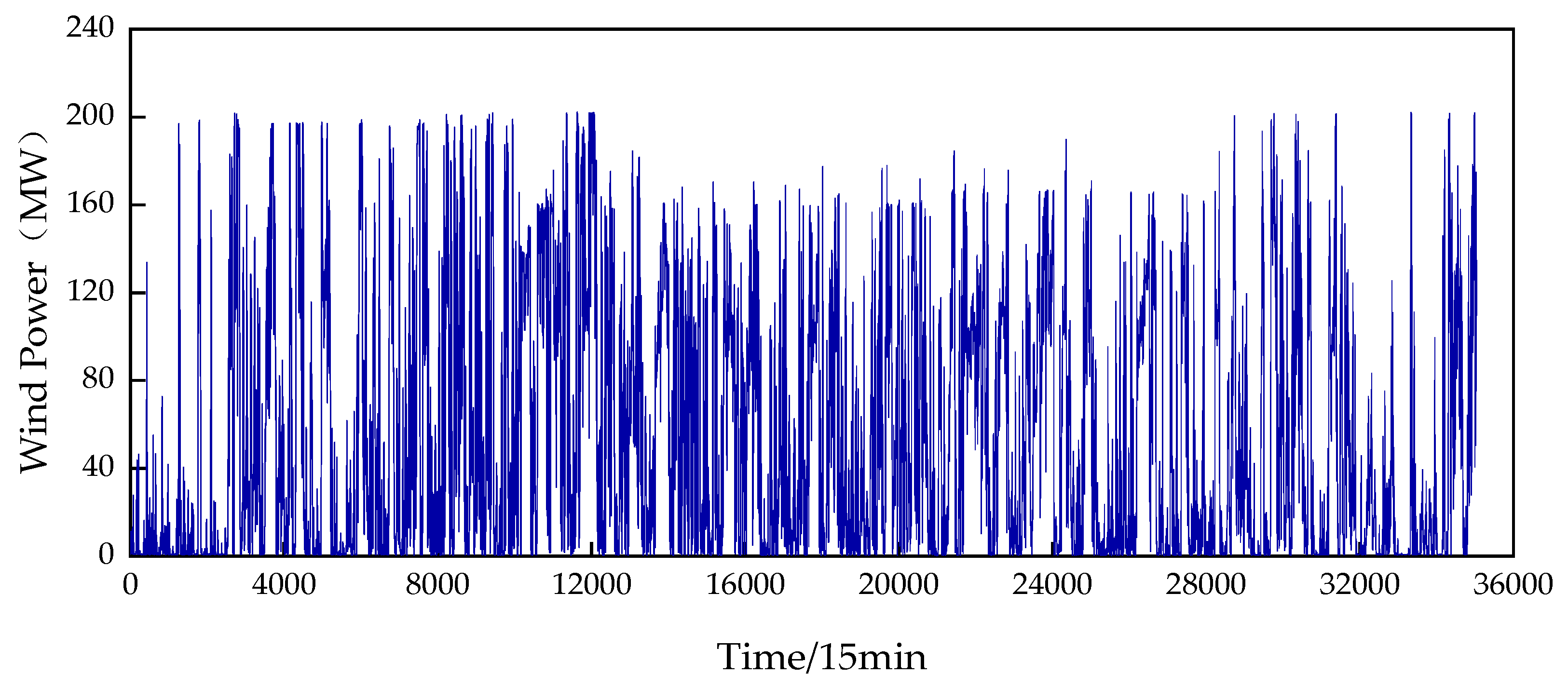
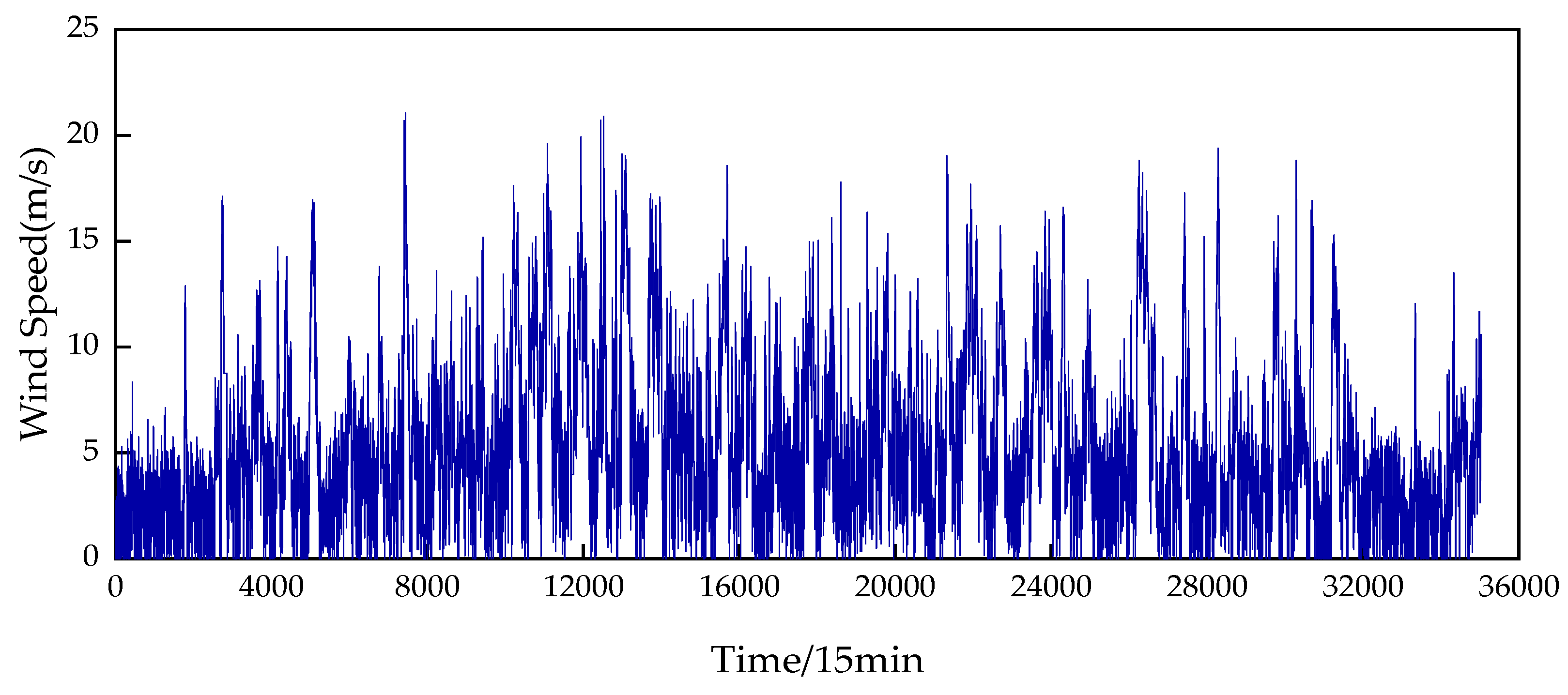
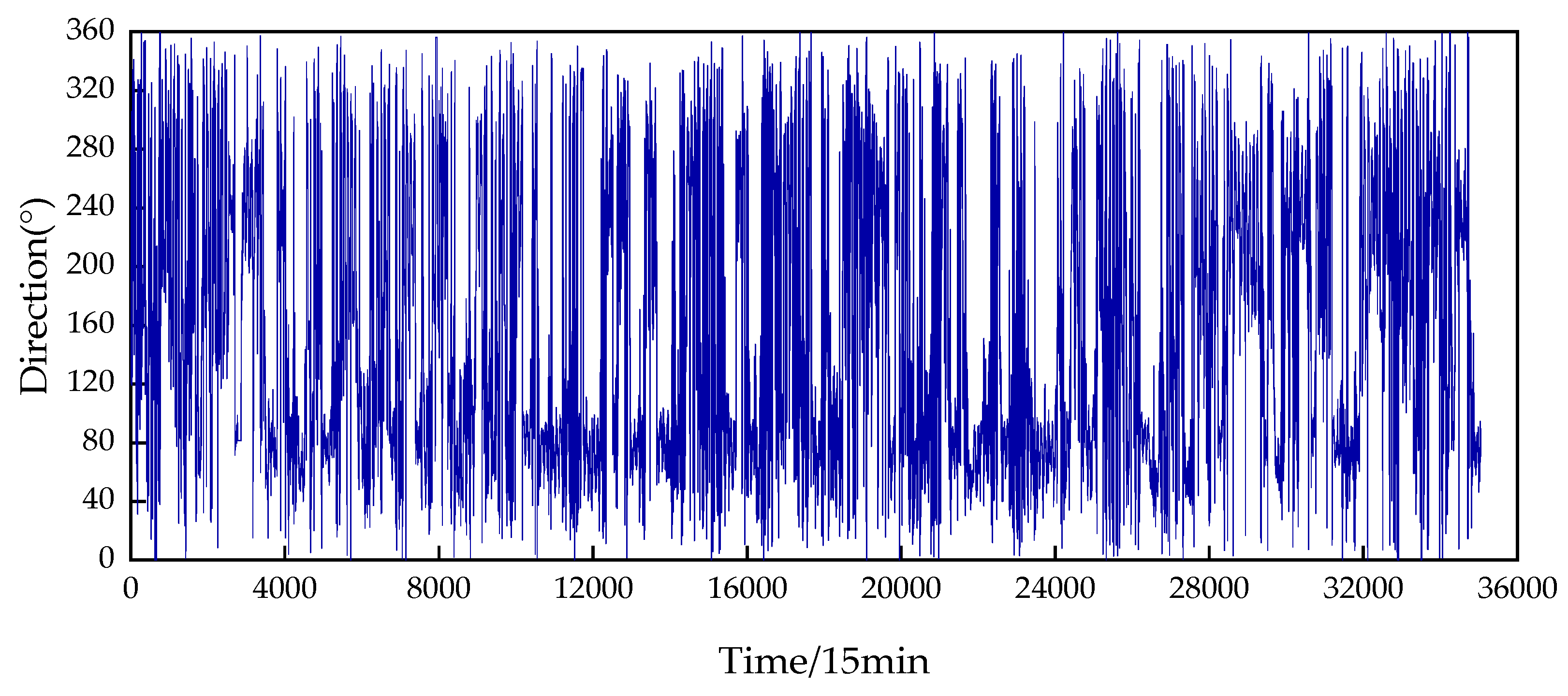
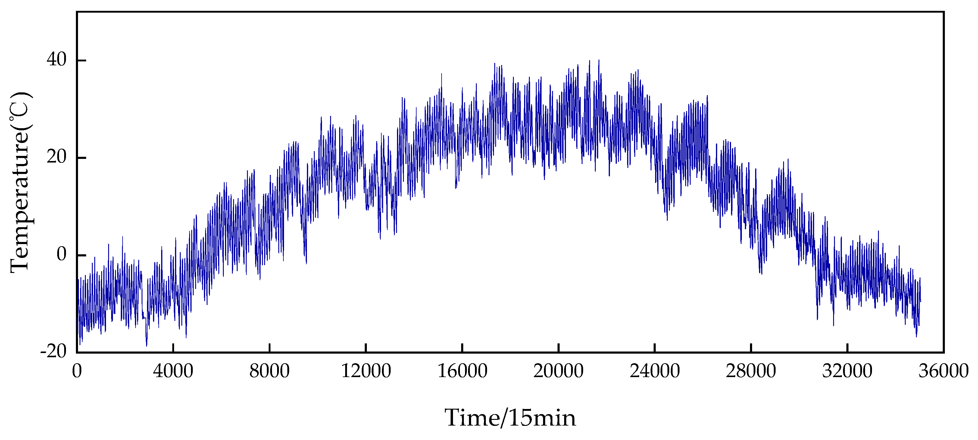
To predict the value of wind power, this paper uses measured data from the first wind farm of Santang Lake, a wind power base in Hami City, Xinjiang Province, China. The wind farm has an installed capacity of 201 MW and is made up of 134 wind turbines rated at 1.5 MW. Data were collected at fifteen-minute intervals from 1 January 2021 to 31 December 2021. In addition, NWP data were used to analyze wind power characteristics, all of which were obtained from https://xihe-energy.com/#climate, accessed on 1 May 2023, and have been placed in Appendix A for specific data. Table 1 shows the summarized values of the collected data.

2.2. Wind Speed-Wind Power Curve

Wind power generation refers to the process in which wind turbines utilize the blades of the wind turbine to convert the kinetic energy of the wind into mechanical energy, which is then converted into electrical energy by the generator. Due to the natural characteristics of wind energy, the wind speed is constantly fluctuating, so the output power of the wind turbine is also constantly fluctuating [21]. In this paper, the Weibull distribution is used to model the uncertainty of wind power and to represent the relationship between the variation of wind speed and wind power [22], as shown in Equation (1):
P w , t = 0 , v < v i , v > v o 1 2 C P ρ S v 3 , v i v v n P w , v n v v o
where C p denotes the wind energy utilization coefficient, which is the ratio of the absorbed wind energy to the initial wind energy; ρ denotes the air density; S denotes the blade contact area; v denotes the wind speed; and vi, vn, and vo denote the cut-in, rated, and cut-out wind speeds, respectively.
To visualize the distribution of wind speed and power during the actual operation of the wind turbine, the wind speed–wind power (v-P) scatter plot of the wind farm can be drawn, as shown in Figure 1. The data chosen for Figure 1 are based on the data from the Xinjiang wind farm, which has an overall installed capacity of 201 MW. From Figure 1, it can be seen that the wind power data are volatile and uncertain. At low wind speeds, wind power is minimal, whereas at high wind speeds, wind power rises and peaks at a certain point, and then decreases as wind speed continues to increase [23]. Consequently, wind power generation systems must have accurate data for predicting wind power.

2.3. Wind Power Data Outlier Handling

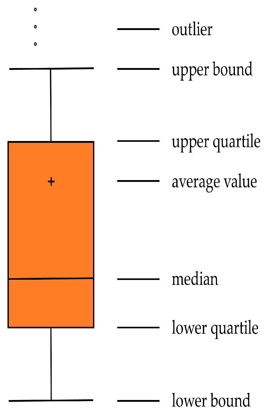
In the actual wind power prediction, there are some data anomalies in wind farms due to wind abandonment, power outages, and measurement device failures, so the anomalous data need to be dealt with. The box-and-line plot is based entirely on actual data, and it provides a realistic and intuitive picture of the distribution pattern of the data. In addition, the box-and-line plot uses interquartile spacing as a criterion for judging outliers, which makes its identification of outliers more objective and has certain advantages, as shown in Figure 2 for the box-and-line plot [24]. In this paper, a mathematical model based on the principle of quartiles is used to process the anomalous data of wind farms, to find out the anomalous values of the data outside the upper and lower boundaries, and to choose the average value method to correct the data, as shown in Equation (2):
A t = A t 1 + A t + 1 2
where A t is the outlier, A t 1 is the data before the outlier, and A t + 1 is the data after the outlier.

2.4. Normalization of Wind Power Data

For time series data, there is always the problem of missing data in the original data, and during the data preprocessing phase, the missing values should be filled in first to ensure the data’s integrity [25]. To satisfy the data structure of the input layer of the convolutional neural network more effectively, in this paper, the time series data are transformed into one-dimensional data, so that the data have the same metric scale, and the data in the range of [0, 1] are normalized. As shown in Equation (3):
x 0 = x t x min x max x min
where x 0 is the normalized data; x t is the actual value; and x min and x max are the minimum value and maximum value of each type of data, respectively.
When the neural network makes a prediction, the prediction needs to be restored to the original power interval according to the inverse normalization formula as shown in Equation (4) [26].
x = x 0 ( x max x min ) + x min
where x is the inverse normalized value.

2.5. CEEMDAN-Based Wind Power Data Decomposition

Due to the unpredictability of wind power data, which is directly incorporated into the prediction model, noise interference in the data may reduce the accuracy of the prediction. Consequently, the application of plausible data classification can provide highly credible training data for prediction models, thereby reducing prediction errors and enhancing prediction accuracy [27].
Additionally, the impact of external conditions, such as meteorological and environmental factors, on the wind farm may result in data anomalies. When using wind power data for modeling and analysis, it is necessary to preprocess the data to eliminate unnecessary disturbances and errors [28]. Many researchers use empirical mode decomposition (EMD) [29] to pre-process wind power data, and EMD can decompose the data to extract the intrinsic mode function (IMF) at various frequencies. The processing and analysis of IMF at various time scales can reveal wind power data’s hidden feature information [30].
However, the EMD method generates problems with modal mingling and incomplete decomposition when decomposing, so we present the CEEMADN method. Based on the EMD method, the CEEMDAN method adaptively superimposes a new white noise into its residual component whenever a new IMF is derived from the decomposition until the residual component is no longer decomposable and the decomposition concludes [31]. The following is the specific procedure of the CEEMDAN method for decomposing wind power data.
  • Adding white noise w i n with a mean value of 0 to the original signal x n , the data signal of the i-th experiment is
    x i n = x n + ε w i n   i = 1 , 2 , , I
    where ε is the weight coefficient of white noise; i = 1 , 2 , , I is the number of trials.
  • The signal x i n is decomposed by EMD, and the first modal component I M F 1 n and the first residual component are obtained after decomposition as r 1 n .
    I M F 1 n = 1 I i = 1 I I M F 1 i n
    r 1 n = x n I M F 1 n
  • Assuming that E K is the modal operator, the second modal component I M F 2 n is obtained by adding white noise ε 1 E 1 w i n to the residual component r 1 n and then performing EMD decomposition.
    I M F 2 n = 1 I i = 1 I E 1 r 1 n + ε 1 E 1 w i n
    where ε 1 is the white noise weight coefficient, w i n is the white noise produced during the ith processing, r 1 n is the first modal component, and E 1 is the modal operator. I represents the total amount of decomposition sequences. The second residual component remaining is denoted as r 2 n .
    r 2 n = r 1 n I M F n
  • Using the above method yields the kth modal component I M F k + 1 n and the kth residual component r k n .
    I M F k + 1 n = 1 I i = 1 I E 1 r k n + ε k E k w i n
    r k n = r k 1 n I M F k n
  • Using the above steps until the CEEMDAN stopping condition is met, the final data decomposition is
    x n = k = 1 K I M F k n + R n
    where R n is the residual component.
Decomposition of wind power data using the CEEMDAN algorithm can transform unstructured raw data into a more stable, ordered sequence, thereby capturing more wind power data features. If each subcomponent of the CEEMDAN decomposition is predicted individually and explicitly, this will increase computation time and slow prediction.

2.6. Reconstruction of Wind Power Sequences Based on Sample Entropy

Richman and Moorman’s SE is an enhanced version of the approximate entropy (AE) algorithm [32]. The value of the sample entropy represents the time series’ complexity. The higher the value of sample entropy, the more complicated the time series, and vice versa. SE can therefore effectively reduce the complexity of computation and modeling by combining sequences with similar entropy values for prediction, thus improving prediction accuracy and efficiency [33]. Here is how to calculate the sample entropy:
There exists a time series Z = z 1 , z 2 , z N which forms an m-dimensional vector, Z m i = z i , z i + 1 , , z i + m 1 b. Define the distance between Z i and Z j in the sequence as d m Z i ,   Z j denoted as:
d m Z i ,   Z j = max k 0 , m 1 z i + m z j + m
Given a similarity tolerance r, for each value of i, count d m Z i ,   Z j < r , and the ratio of its ratio to the total number of distances is B m r . Then, the definition of sample entropy is
S a m p E n m , r = lim N ln B m r ln B m + 1 r
When N is finite, the calculation can be performed using Equation (15):
S a m p E n m , r , N = ln B m r ln B m + 1 r
Reconstructing the wind power series by sample entropy can reduce the error caused by repeated modeling and merge the sub-series with similar entropy values into a new series based on the sample entropy value. The reconstructed components are then processed for RF feature selection to eliminate the redundant features of the wind power series and improve the prediction performance [34].

3. Wind Power Prediction Model Based on BiLSTM Neural Network

3.1. Gray Relation Analysis

Gray Relation Analysis (GRA) is an algorithm used to analyze the degree of similarity between parameters. The essence of this algorithm is to analyze the similarity between the trends of each parameter over time, that is, to calculate the degree of correlation between the rate of change of the values of each parameter between two adjacent moments. The closer the interrelationship between the data, the greater the gray correlation.
The value of wind power is influenced by several factors, including meteorological factors and the internal structure of the wind turbine. To calculate the effect of these factors on wind power, a gray correlation analysis was employed. Calculating the degree of correlation between various factors and wind power, the method determines the magnitude of each factor’s influence on wind power and selects several factors with the highest correlation as input parameters for prediction. This method can effectively improve the accuracy of predictions, investigate the laws and characteristics underlying wind power data, and avoid the errors caused by an excessive amount of balanced data input [35]. The specific analysis steps are as follows:
Firstly, the wind power data sequence obtained after normalization according to Equation (3) is
x 0 = x 0 1 , x 0 2 , , x 0 n
The normalized data series for each factor are as follows:
x i = x i 1 , x i 2 , , x i n
Calculate the gray correlation coefficient ξ i k
ξ i ( k ) = min i min k x 0 ( k ) x i ( k ) + ρ max i max k x 0 ( k ) x i ( k ) x 0 ( k ) x i ( k ) + ρ max i max k x 0 ( k ) x i ( k )
where ρ is the resolution factor, and ρ = 0.5 is taken in this paper.
The gray relation between the series of each influence factor and the wind power data series is calculated, γ i .
γ i = 1 n k = 1 n ξ i k
The closer the value of γ i is to 1, the better the correlation. The influencing factors were ranked according to their correlation.

3.2. LSTM Neural Network

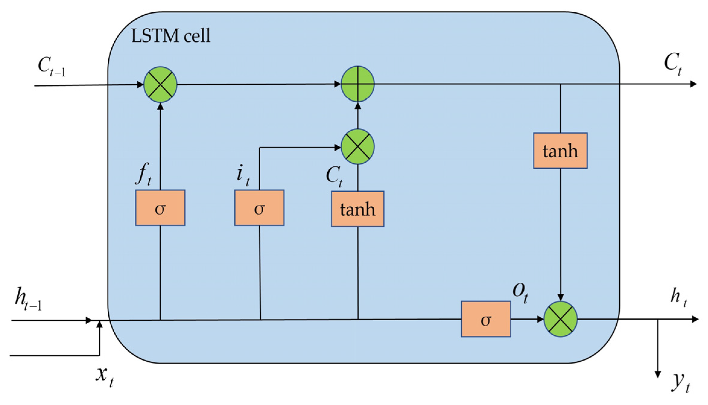
LSTM is a temporal recurrent neural network based on a recurrent neural network (RNN). LSTM introduces three gates, the forgetting gate, input gate, and output gate, to solve the gradient disappearance and gradient explosion problems existing in RNN [36], and its structure is shown in Figure 3. LSTM can fully exploit the wind power information when backpropagation is performed, allowing the wind power prediction model to continue learning at multiple time steps to reduce the error of wind power prediction and improve its accuracy. For a given moment t, the operator in the LSTM cell has the following equation:
h t = f h t 1 , X t
i t = σ W i h t 1 , X t + b i
f t = σ W f h t 1 , X t + b f
o t = σ W o h t 1 , X t + b o
C t = tanh W c h t 1 , X t + b c
S t = f t S t 1 + i t C t
h t = o t tanh S t
where W is the weight of the corresponding gate and memory; b is the bias added when calculating the corresponding gate and memory; S t is the current cell state; C t is the candidate value of the new cell state S t ; h t denotes the output information of the current time series; o t denotes the output gate; f t denotes the forgetting gate; and i t denotes the input gate.

3.3. BiLSTM Neural Network

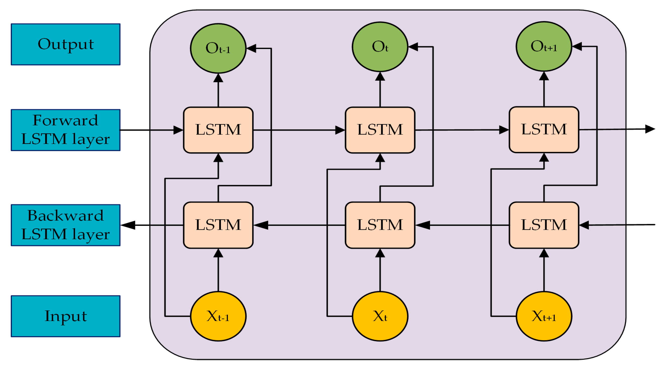
BiLSTM is developed from LSTM. The BiLSTM can mine time series data from both the past and the future since it comprises two LSTMs running in reverse parallel and containing all the information in both the forward and reverse directions. The structure diagram is shown in Figure 4.
The input layer of BiLSTM feeds the input data into the forward network and the backward network, respectively, and the output of the network is spliced and processed, and the output is shown in Equation (27). The last output of the forward and backward is stitched together and used as the input to the next layer, and the output dimension is set to two times the input dimension to minimize the complexity of the model.
h j = h j , h j   j = 1 , 2 , , n 1
where h j denotes the final output result of the jth data after forward and backward transmission, and j = 1 , 2 , , n 1 is the total number of input data.

3.4. Wind Power Data Residual Correction Based on MC

MC is a Markov process that considers both time and state discretization. MC describes a sequence of states where the state at a given moment is only related to a finite number of preceding states. In addition, the states and times described by the model are discrete, meaning that only a limited number can be selected [37], so it is suitable for correcting prediction problems with volatility.
Wind power data are discrete time series, and the probability of wind power is affected by random factors such as wind speed and temperature, resulting in a decrease in model accuracy [38]. This paper uses MC to correct the error situation of the forecast day based on the error situation of the historical day so that the corrected wind power output is closer to the actual value [39]. In this paper, using a Markov-chain-based method, historical data are used as input parameters, the possible prediction error states for each period can be derived via chain derivation, and the prediction results are then adjusted accordingly. This method can effectively reduce the prediction bias and improve the prediction accuracy. The steps of Markov-chain-based prediction error correction are as follows:
  • Calculation of wind power error series:
    β n = q i q i ,   n = 1 , 2 , , N
    where q i a represents the actual historical wind power data of sample point n; q i represents the predicted value of sample point n derived from the prediction model; and N represents the number of sample points.
  • The sample means x ¯ and standard deviation δ of the error series are computed, and the wind power error series is subdivided into five intervals using the mean-variance state division method by the MC:
    H 1 = min e s , s , x ¯ δ H 2 = x ¯ δ , x ¯ 0.5 δ H 3 = x ¯ 0.5 δ , x ¯ + 0.5 δ H 4 = x ¯ + 0.5 δ , x ¯ + δ H 5 = x ¯ + δ , max e s , s
  • Compute the k-step state transfer matrix P s , where P i j s is
    P i j s = M i j s / M i
    where P i j s is the probability that state H i transfers to the state H j after s steps, M i j s is the number of times state H i transfers to state H j after s steps, and M i is the total number of times state H j occurs. Then the s-step state transfer probability matrix can be expressed as
    P ( s ) = p 11 ( s ) p 12 ( s ) p 15 ( s ) p 21 ( s ) p 12 ( s ) p 25 ( s ) p 51 ( s ) p 52 ( s ) p 55 ( s ) = P ( 1 ) s
  • Since the wind power error sequence is divided into five intervals, the state where the first five values of the wind power error sequence are located is taken as the initial state, and take the row vector P i ( 5 ) = P i 1 ( 5 ) , P i 2 ( 5 ) , , P i 5 ( 5 ) , i = 1 , 2 , , 5 corresponding to each initial state in the transfer matrix p 5 , thus forming a new probability matrix as
    R = p i 1 ( 1 ) p i 2 ( 1 ) p i 5 ( 1 ) p i 1 ( 2 ) p i 2 ( 2 ) p i 5 ( 2 ) p i ) ( 5 ) p ( 5 ) p i s ( 5 )
  • Take the state corresponding to max P j = i = 1 N p i j ( s ) , i [ 1 , N ] , j [ 1 , N ] , which is also the state to which the error sequence is most likely to be transferred, to be the state of that corrected error sequence. The corrected value of this error is
    β ˜ n = β n + 0.5 E 1 + E 2
    where E1 and E2 are the upper and lower bounds of He for the residual state interval to be corrected.
  • Correction of the predicted wind power series for the day to be forecast is
    q i = q i + β ˜ n
    where q i and q i are the predicted wind power values before and after correction, respectively.

3.5. The Model’s Evaluation Standards

Four indicators are selected to evaluate the short-term wind power prediction results: root mean square error (RMSE), mean absolute error (MAE), mean absolute percentage error (MAPE), and accuracy rate ( R A R ). The smaller the values of RMSE, MAE, and MAPE, the smaller the prediction error of the model, and the closer the value to 1, the better the model performance. The formula for calculating the four indicators is as follows:
R M S E = 1 N i = 1 N y i y ^ i 2
M A E = 1 N i = 1 N y i y ^ i
M A P E = 1 N i = 1 N y i y ^ i y i × 100 %
R A R = 1 i = 1 N y i y ^ i 2 i = 1 N y ¯ i y ^ i 2
where N is the number of prediction series; y i and y ^ i are the measured and predicted values of wind power, respectively; and y ¯ i is the average value of measured power.

4. CEEMDAN-SE-BiLSTM-MC Prediction Model Building

In this study, a CEEMDAN-SE-BiLSTM-MC-based wind power short-term prediction model is proposed for the characteristics of intermittent and stochastic fluctuations in wind power data. The prediction process is shown in Figure 5, and the process is as follows:
  • Using the CEEMDAN algorithm, the raw wind power data are decomposed to derive several modal components and residual components. The sample entropy values of each component are calculated, and the components with similar entropy values are combined and reconstructed to form a new power component sequence.
  • The correlation value of each wind power reconstruction power component is calculated according to the gray correlation algorithm, and the influence value with a gray relation greater than 0.9 is selected as input.
  • Each component is divided into a training set and a test set, and the reconstructed wind power components are predicted separately using the BiLSTM network, and the overall wind power prediction is obtained by summing up all the predicted values.
  • The prediction error between the historical wind power and the predicted power is calculated, and the preliminary prediction results are corrected using Markov chains to obtain the final predicted wind power.
  • The wind power prediction results are contrasted with the actual measured values, and then the prediction errors are analyzed.

5. Example Simulation Analysis

5.1. Experimental Data

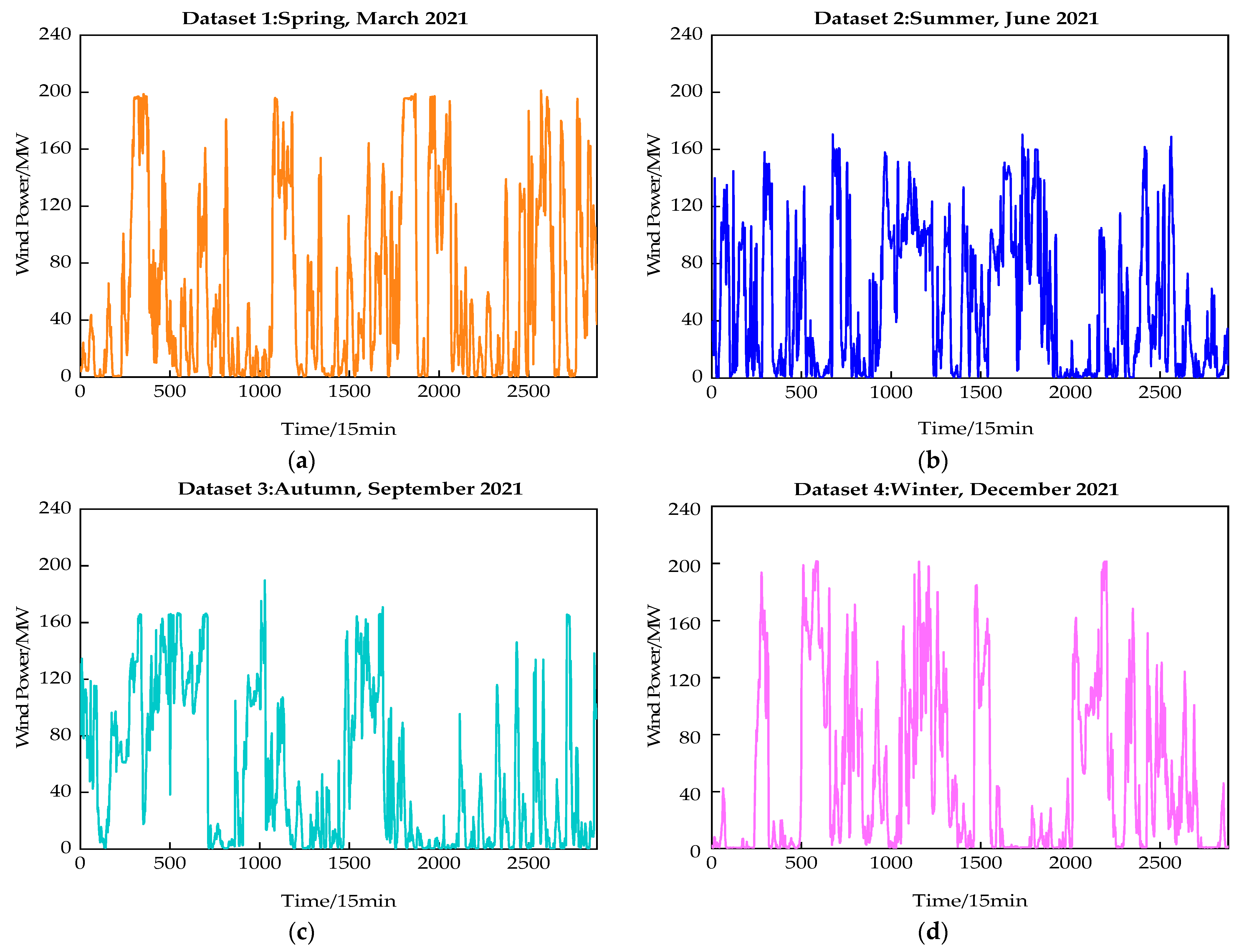
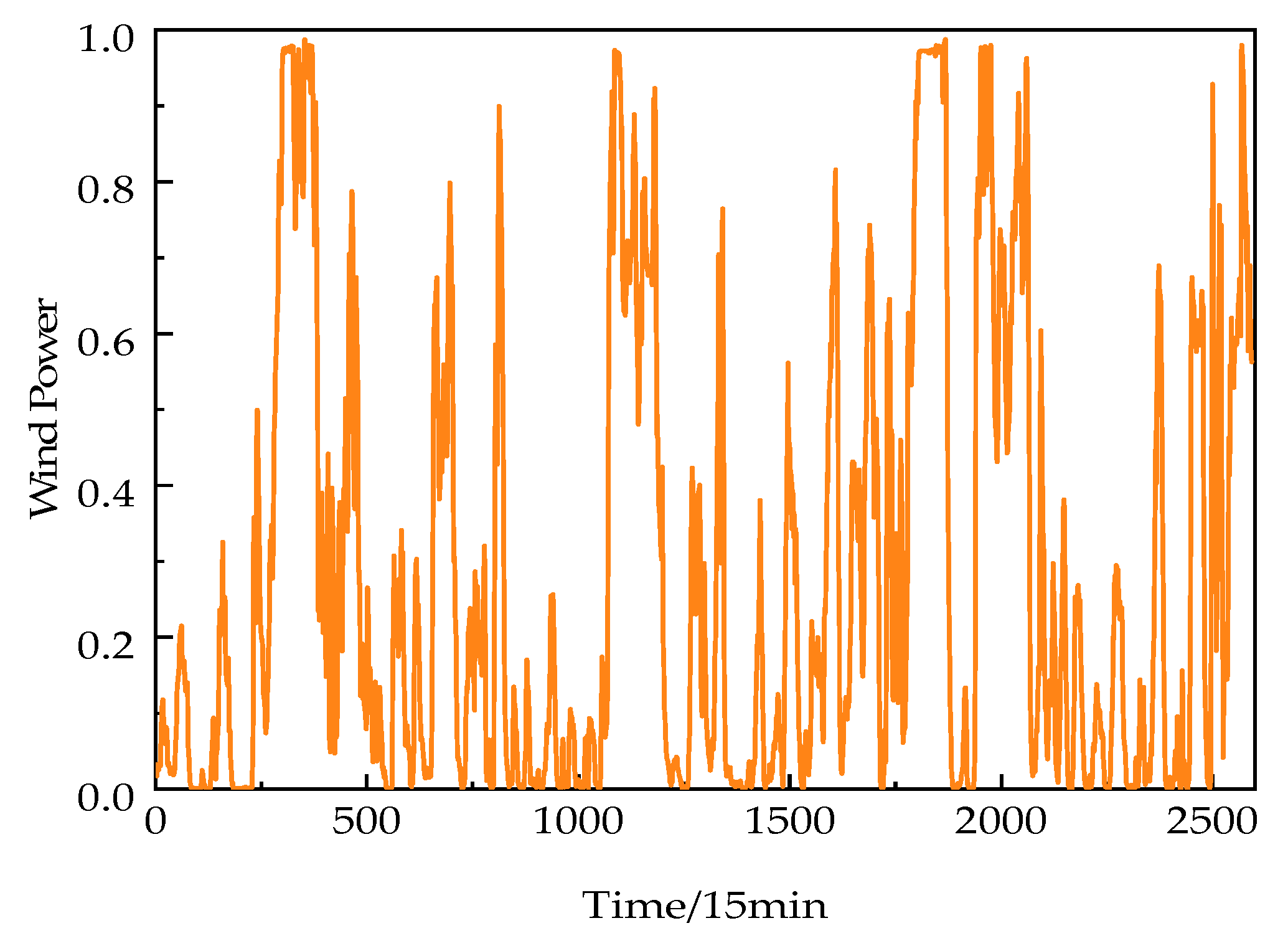
In this paper, the wind power data are sourced from a wind farm in Xinjiang, and to verify the effectiveness of the proposed model, four sets of wind power data from different seasons are selected as the input of the neural network, which are March 1–March 30, June 1–June 30, September 1–September 30, and December 1–December 30, as shown in Figure 6, to test the prediction performance of the model in different seasons. The temporal resolution of each data set is 15 min, and the first 2592 data of each data set are used as the training set of the prediction model according to the division of 9:1, and the remaining 288 data are used as the test set of the prediction model.
Table 2 shows the statistical information for each data set, which indicates that wind power displays a high degree of volatility and non-stationarity, with the power output being greater in the spring and winter and less in the summer and fall.
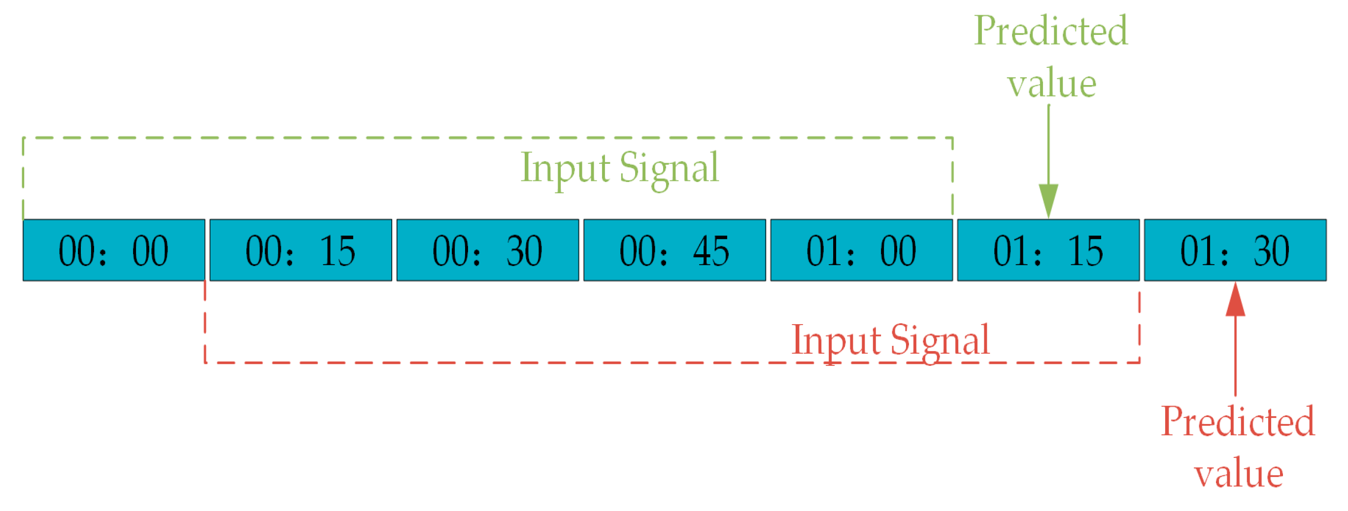
In this paper, the sliding window prediction method is used, and the schematic diagram of sliding window prediction is shown in Figure 7. At 1:00, the data from 00:00 to 01:15 is input, and at 1:30, the predicted wind power is output. The model is implemented within the deep-learning framework TensorFlow with the Adam optimizer, 100 iterations, a batch size of 32, a convolutional kernel size of 3, a learning rate of 0.001, and a deactivation rate of 0.1.

5.2. Results of GRA

Using the March data as an example, the data are first normalized to narrow the gap between the data in terms of magnitude to avoid too large an error in the training, and the results after data normalization are shown in Figure 8.
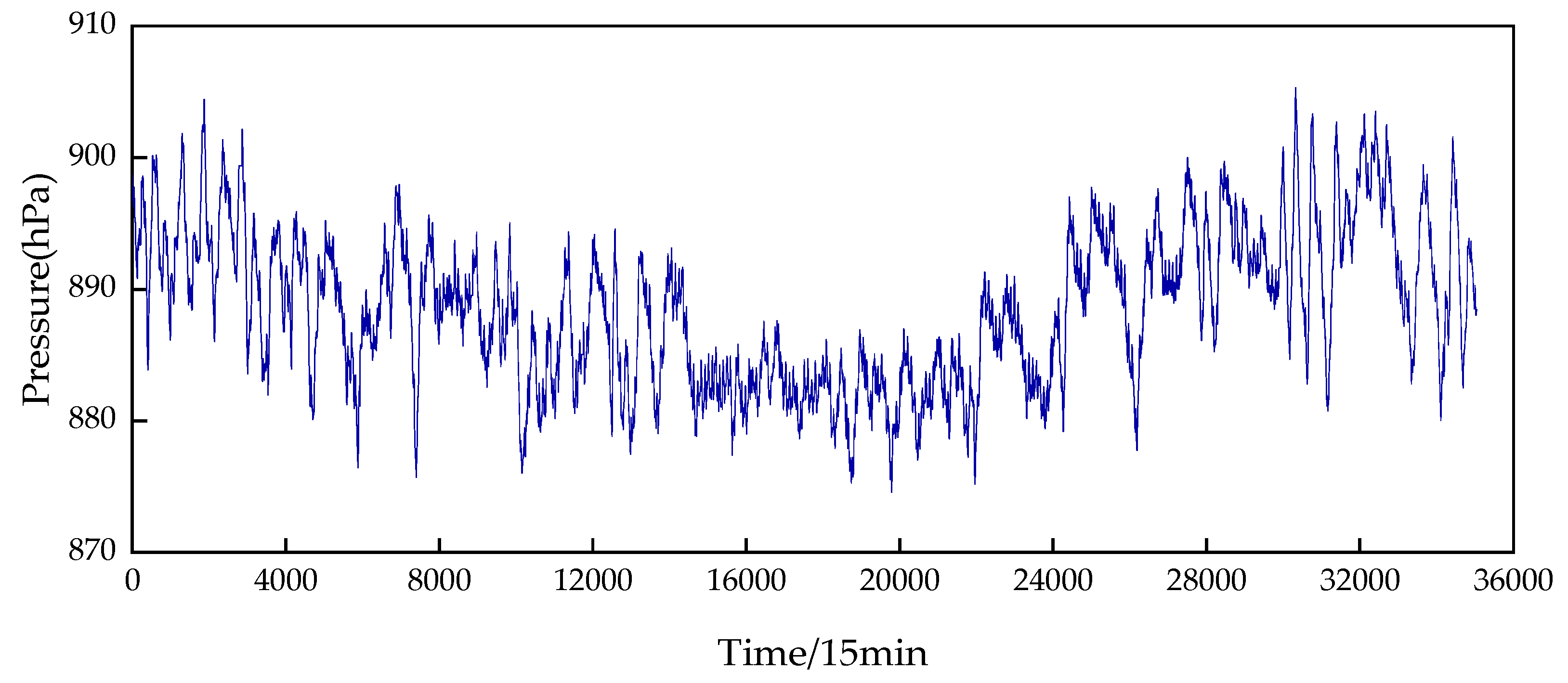
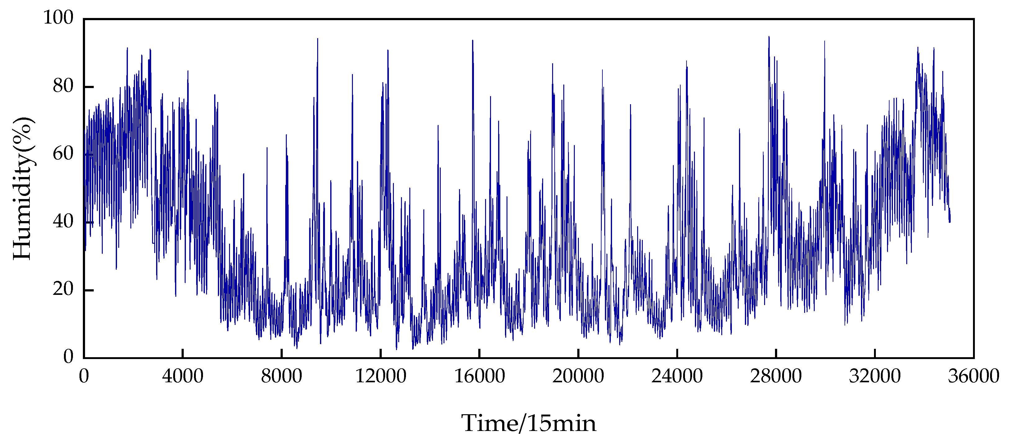
The calculations in this paper are based on actual monitoring data collected from a wind farm in the Xinjiang region of China in 2021. Power, wind speed, wind direction, temperature, air pressure, and humidity were selected as sample data for data relation analysis. Figure 9 depicts the relation analysis of each data type with the power data, which correspond to power, wind speed, wind direction, temperature, air pressure, and humidity with relation coefficients of 1, 0.932, 0.917, 0.908, 0.895, and 0.892, respectively. By comparing the high and low relations, power, wind speed, wind direction, and temperature will be selected as the prediction model input data in this paper.

5.3. Data Pre-Processing Results

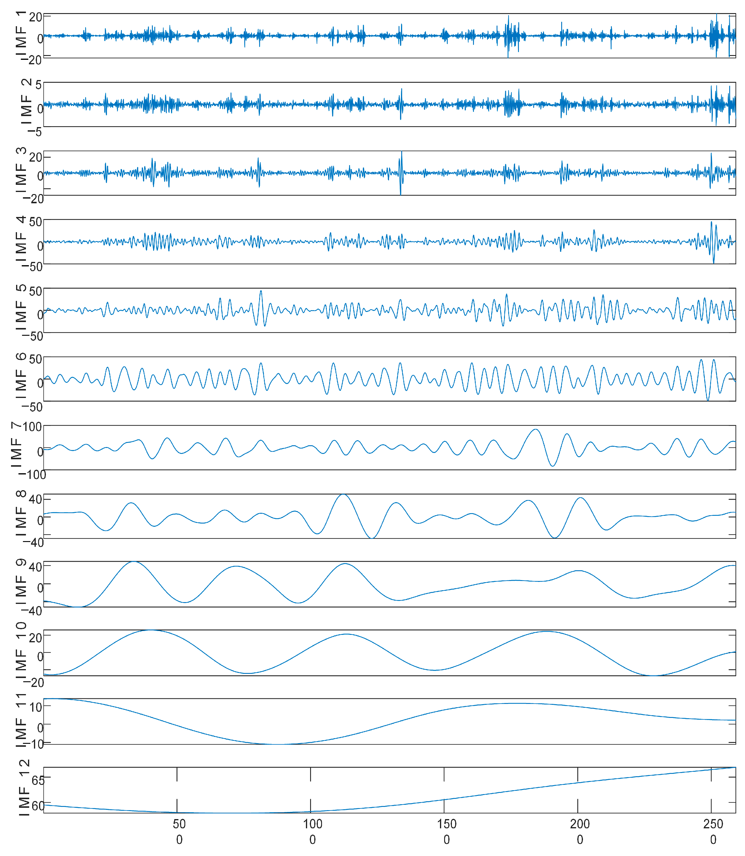
In this paper, the CEEMDAN algorithm is used to preprocess the wind power series with the added white noise standard deviation of 0.2 and the number of additions of 500, using the March data as an example, the resulting power components IMF1-IMF12 and IMF12 are the residual components, and the decomposition diagram is shown in Figure 10. It can be seen that the CEEMDAN algorithm decomposes the wind power series into multiple modal components with different frequency period characteristics, which is convenient for analyzing the hidden information in the data and overcoming the shortcomings of the original wind power series which are volatile and non-smooth.
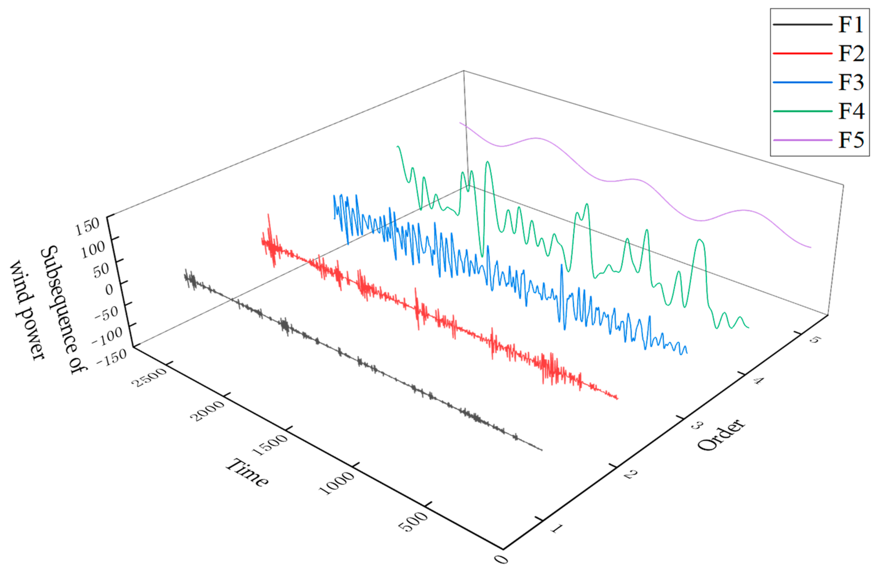
In this study, the sample entropy values of each power component were calculated to analyze the complexity and confusion of the data for each wind power component, and the results are presented in Table 3. According to the data in Table 3, it can be seen that the sample entropy value of each component decreases as the frequency of each IMF component decreases, which indicates that the complexity of the sample is decreasing and proves that the sample entropy value is valid. The quantities with close sample entropy values are combined to form a new reconstructed component to reduce the complexity of the computation. Table 4 presents the correspondence between the reconstructed power components and the original power components. By replacing the original power component sequence with a recombined power component sequence, the reconstructed power component sequence is used as the new prediction target.
Figure 11 depicts the results derived by reconstructing the CEEMDAN decomposed sequences based on Table 4’s results, and it can be seen that the sample entropy can reduce the redundancy of the data.

5.4. Analysis of Prediction Results

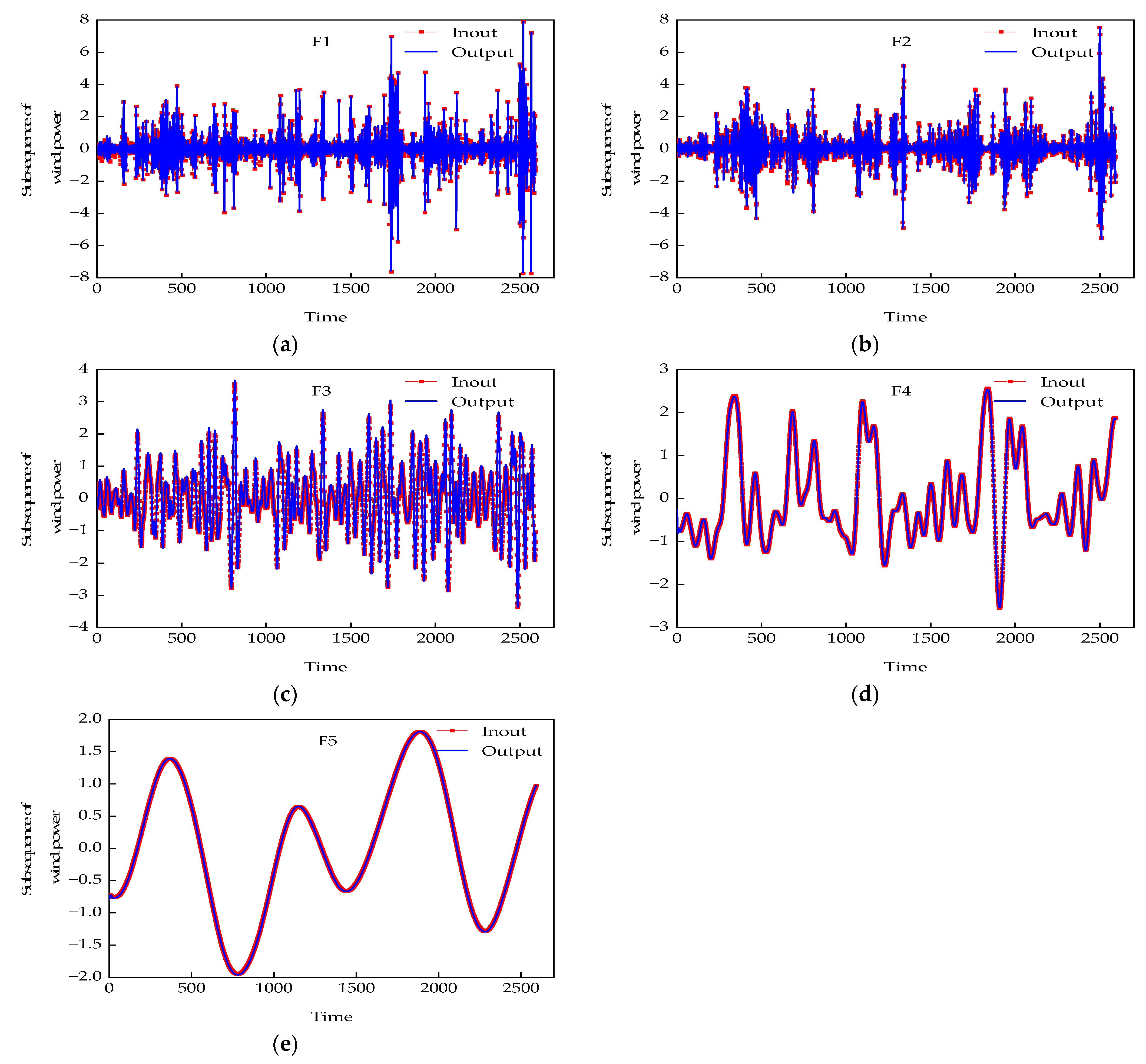
Figure 12 illustrates the results of training the five reconstructed components independently with BiLSTM. The red color represents the input data of the model, and the blue color represents the output data of the model. Figure 11 demonstrates that BiLSTM is capable of predicting the next value of each reconstructed component on time and that the trained BiLSTM network has excellent generalization ability and can be used for future wind power prediction.
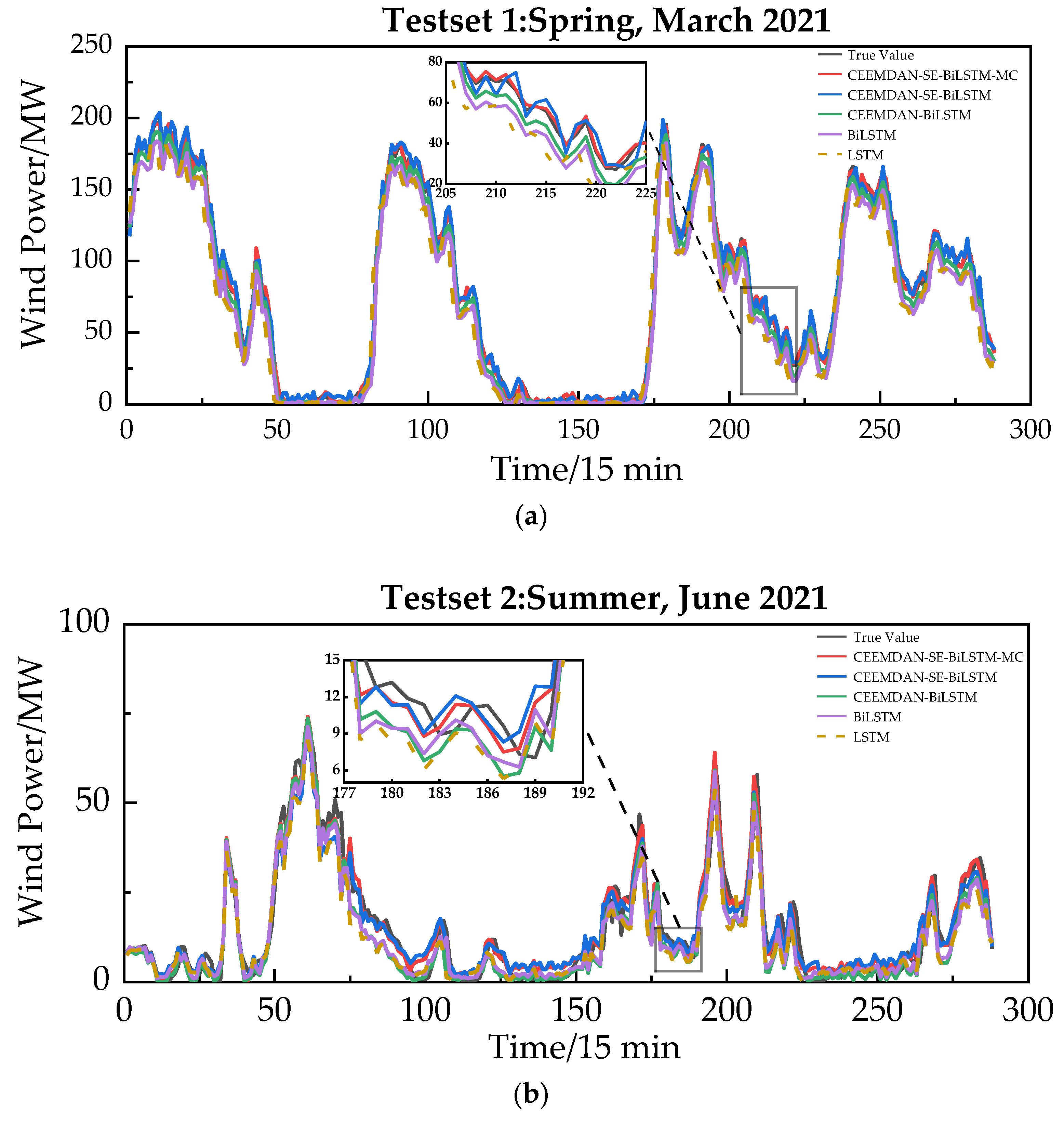
To verify the predictive effect of the model proposed in this study, five different control models were selected for comparison tests in the test set; these are CEEMDAN-SE-BiLSTM-MC, CEEMDAN-SE-BiLSTM, CEEMDAN-LSTM, BiLSTM, and LSTM, respectively. The predicted results are shown in Figure 13.
Figure 13 illustrates that the prediction curve of the prediction algorithm utilized in this paper has a superior fit and higher prediction accuracy. Table 5 illustrates the error results for each model.
As shown in Table 5, the models used in this paper have the highest prediction accuracy; the RMSE was 1.792 MW, 3.724 MW, 1.476 MW, and 1.429 MW in March, June, September, and December, respectively; the MAE was 1.479 MW, 2.826 MW, 1.275 MW, and 1.015 MW; the MAPE was 0.202 MW, 0.431 MW, 0.419 and 0.113 MW in March, June, September, and December, respectively., and the R A R was 0.999 MW, 0.953 MW, 0.999 MW, and 0.997 MW in March, June, September, and December, respectively. It can be seen that the CEEMDAN-SE-BiLSTM-MC model has a large prediction error when predicting the wind power of this power plant in June. This is because the wind power data of this wind farm during the summer is more volatile, but the model presented in this paper can still accurately anticipate it, demonstrating the model’s strong ability to fit the data.
From an examination of Table 4 and Figure 12, the following inferences can be made:
  • In June, when comparing the evaluation metrics of BiLSTM and CEEMDAN-BiLSTM, the RMSE, MAE, and MAPE of CEEMDAN-BiLSTM decreased by 3.5%, 32.2%, and 20.5%, respectively, while the R A R increased by 0.7%. In the remaining three months, the forecasting metrics improved due to the ability of the decomposition algorithm to decompose the raw data into multiple regular and smoother data, making it simpler for the model to capture more valuable information and produce more accurate forecasting results.
  • For the prediction model with sample entropy added, the RMSE, MAE, and MAPE of the model with sample entropy added are smaller than those of the model without sample entropy added, and the R A R is greater than that of the model without sample entropy added, compared with the prediction model without sample entropy added. Observably, the sample entropy reduces the error of the BiLSTM model’s prediction results and improves its prediction performance.
  • Taking the March data as an example, the RMSE, MAE, MAPE, and RAR of the BiLSTM model are smaller than those of the LSTM model, and the R A R is improved by 3.6%, so the BiLSTM model has higher prediction accuracy in the experiment compared with the LSTM model, and the unique network architecture of the BiLSTM model has some advantages in the temporal prediction.
  • In addition, comparing the CEEMDAN-SE-BiLSTM-MC model with the CEEMDAN-SE-BiLSTM model, it can be seen that all four evaluation metrics of the MC error correction method outperform the model without using the error correction method. This illustrates the superiority of this error correction algorithm, which can further improve the prediction accuracy of the model while retaining the good robustness of the CEEMDAN-SE-BiLSTM model.
From the preceding analysis, it can be concluded that the CEEMDAN-SE-BiLSTM-MC model better fits the wind power data and has a superior wind power prediction effect.

6. Conclusions

This paper proposes a short-term wind power prediction model based on the CEEMDAN-SE-BiLSTM-MC algorithm for complex and evolving wind power data. First, the CEEMDAN algorithm is used to decompose the sequences, then the decomposed sequences are merged using SE to reduce the computational complexity, then the reconstructed subsequences are predicted using a BiLSTM neural network to superimpose the prediction results of each sequence, and then the total predicted power of the superimposed sequences is corrected by MC. Through example validation, the following conclusions were drawn:
  • The original wind power data were decomposed and reconstructed using CEEMDAN-SE. Compared with the unprocessed model, the model using CEEMDAN-SE had an 8% reduction in RMSE and a higher prediction accuracy in the middle of June, which indicates that CEEMDAN-SE can effectively process the wind power data and reduce the degree of redundancy of the data.
  • An improved LSTM neural network model is used to MC correct the predicted data, which effectively reduces the error of the predicted data and improves the accuracy of the prediction.
  • The CEEMDAN-SE-BiLSTM-MC model proposed in this paper is compared with other models, and the model is evaluated by four kinds of indexes using wind power data from four different months, which demonstrates the accuracy of this paper’s model in the prediction of wind power and has a better prediction effect compared with other prediction models.
Although the overall performance of the method presented in this paper is superior, the prediction results of individual points contain some errors when compared to other methods; therefore, the reasons for this must be investigated further in the future, and solutions are provided. Secondly, this paper only uses the historical data of a single wind farm to construct the model; in the future, data from multiple wind farms can be utilized for validation to improve the practical application value of the model. At the same time, to better serve the power dispatching work, the model can be software materialized to facilitate its use in engineering practice and provide strong support for the power dispatching work.

Author Contributions

Conceptualization, J.H. and L.H.; methodology, Y.L.; formal analysis, Y.W. (Yanyang Wang); investigation, Y.W. (Yu Wang); data curation, Z.L.; writing—original draft preparation, Y.L.; writing—review and editing, J.H. All authors have read and agreed to the published version of the manuscript.

Funding

This research received no external funding.

Data Availability Statement

Not applicable.

Conflicts of Interest

The authors declare no conflict of interest.

Abbreviations

CEEMDANComplementary ensemble empirical mode decomposition with adaptive noise
SESample entropy
BiLSTMBidirectional long short-term memory network
MCMarkov chain
NWPNumerical weather prediction
IMFIntrinsic mode function
EMDEmpirical mode decomposition
GRAGray Relation Analysis
RMSEResults root mean square error
MAEMean absolute error
MAPEMean absolute percentage error
RARAccuracy rate

Appendix A

Figure A1. Wind power versus time graph.
Energies 16 05476 g0a1
Figure A2. Wind speed versus time graph.
Energies 16 05476 g0a2
Figure A3. Direction versus time graph.
Energies 16 05476 g0a3
Figure A4. Temperature versus time graph.
Energies 16 05476 g0a4
Figure A5. Pressure versus time graph.
Energies 16 05476 g0a5
Figure A6. Humidity versus time graph.
Energies 16 05476 g0a6

References

  1. Liu, L.; Liu, J.; Ye, Y.; Liu, H.; Chen, K.; Li, D.; Dong, X.; Sun, M. Ultra-short-term wind power forecasting based on deep Bayesian model with uncertainty. Renew. Energy 2023, 205, 598–607. [Google Scholar] [CrossRef]
  2. Cheng, K.; Peng, X.X.; Xu, Q.Y.; Wang, B.; Liu, C.; Che, J.F. Short-term Wind Power Prediction Based on Feature Selection and Multi-level Deep Transfer Learning. High Volt. 2022, 48, 497–503. [Google Scholar]
  3. GWEC. The Global Wind Report. 2022. Available online: https://gwec.net/global-wind-report-2022/ (accessed on 1 May 2023).
  4. Cui, Y.; Wang, Y.J.; Huang, Y.H.; Wang, Z.; Wang, M.C. Closed-loop Wind Power Ultra-short-term Forecasting Strategy Based on Multi-attention Framework and Guided Supervised Learning. Proc. CSEE 2023, 43, 1334–1346. [Google Scholar]
  5. Tammelin, B.; Vihma, T.; Atlaskin, E.; Badger, J.; Fortelius, C.; Gregow, H.; Horttanainen, M.; Hyvonen, R.; Kilpinen, J.; Latikka, J.; et al. Production of the Finnish Wind Atlas. Wind. Energy 2013, 16, 19–35. [Google Scholar] [CrossRef]
  6. Wang, K.J.; Qi, X.X.; Liu, H.D.; Song, J.K. Deep belief network based k-means cluster approach for short-term wind power forecasting. Energy 2018, 165, 840–852. [Google Scholar] [CrossRef]
  7. Couto, A.; Estanqueiro, A. Enhancing wind power forecast accuracy using the weather research and forecasting numerical model-based features and artificial neuronal networks. Renew. Energy 2022, 201, 1076–1085. [Google Scholar] [CrossRef]
  8. Karakus, O.; Kuruoglu, E.E.; Altinkaya, M.A. One-day ahead wind speed/power prediction based on polynomial autoregressive model. IET Renew. Power Gener. 2017, 11, 1430–1439. [Google Scholar] [CrossRef] [Green Version]
  9. Zhang, Y.G.; Zhao, Y.; Kong, C.H.; Chen, B. A new prediction method based on VMD-PRBF-ARMA-E model considering wind speed characteristic. Energy Convers. Manag. 2020, 203, 112254. [Google Scholar] [CrossRef]
  10. Aasim; Singh, S.N.; Mohapatra, A. Repeated wavelet transform based ARIMA model for very short-term wind speed forecasting. Renew. Energy 2019, 136, 758–768. [Google Scholar]
  11. Chen, H.; Zhang, J.Z.; Tao, Y.B.; Tan, F.L. Asymmetric GARCH type models for asymmetric volatility characteristics analysis and wind power forecasting. Prot. Control. Mod. Power Syst. 2019, 4, 29. [Google Scholar] [CrossRef] [Green Version]
  12. Yildiz, C.; Acikgoz, H.; Korkmaz, D.; Budak, U. An improved residual-based convolutional neural network for very short-term wind power forecasting. Energy Convers. Manag. 2021, 228, 113731. [Google Scholar] [CrossRef]
  13. Liu, D.; Niu, D.X.; Wang, H.; Fan, L.L. Short-term wind speed forecasting using wavelet transform and support vector machines optimized by genetic algorithm. Renew. Energy 2014, 62, 592–597. [Google Scholar] [CrossRef]
  14. Qing, X.Y.; Niu, Y.G. Hourly day-ahead solar irradiance prediction using weather forecasts by LSTM. Energy 2018, 148, 461–468. [Google Scholar] [CrossRef]
  15. Zhu, Q.M.; Li, H.Y.; Wang, Z.Q.; Chen, J.F.; Wang, B. Ultra-short-term prediction of wind farm power generation based on long- and short-term memory networks. Power Syst. Technol. 2017, 41, 3797–3802. [Google Scholar]
  16. Li, Y.; Tang, F.; Gao, X.; Zhang, T.Y.; Qi, J.F.; Xie, J.R.; Li, X.N.; Guo, Y.H. Numerical Weather Prediction Correction Strategy for Short-Term Wind Power Forecasting Based on Bidirectional Gated Recurrent Unit and XGBoost. Front. Energy Res. 2022, 9, 836144. [Google Scholar] [CrossRef]
  17. Liu, Z.F.; Li, X.Y.; Zhao, H.Y. Short-Term Wind Power Forecasting Based on Feature Analysis and Error Correction. Energies 2023, 16, 4249. [Google Scholar] [CrossRef]
  18. Liu, H.; Duan, Z.; Chen, C.; Wu, H.P. A novel two-stage deep learning wind speed forecasting method with adaptive multiple error corrections and bivariate Dirichlet process mixture model. Energy Convers. Manag. 2019, 199, 111975. [Google Scholar] [CrossRef]
  19. Yang, Q.L.; Deng, C.H.; Chang, X.Q. Ultra-short-term/short-term wind speed prediction based on improved singular spectrum analysis. Renew. Energy 2022, 184, 36–44. [Google Scholar]
  20. Qin, G.Y.; Yan, Q.Y.; Zhu, J.Y.; Xu, C.B.; Kammen, D.M. Day-Ahead Wind Power Forecasting Based on Wind Load Data Using Hybrid Optimization Algorithm. Sustainability 2021, 13, 1164. [Google Scholar] [CrossRef]
  21. Huang, C.M.; Chen, S.J.; Yang, S.P.; Chen, H.J. One-Day-Ahead Hourly Wind Power Forecasting Using Optimized Ensemble Prediction Methods. Energies 2023, 16, 2688. [Google Scholar] [CrossRef]
  22. Wang, Z.M.; Liu, W.M. Wind energy potential assessment based on wind speed, its direction and power data. Sci. Rep. 2021, 11, 16879. [Google Scholar] [CrossRef] [PubMed]
  23. Etemadi, M.; Abdollahi, A.; Rashidinejad, M.; Aalami, H.A. Wind Turbine Output Power Prediction in a Probabilistic Framework Based on Fuzzy Intervals. Iran. J. Sci. Technol. Trans. Electr. Eng. 2021, 45, 131–139. [Google Scholar] [CrossRef]
  24. Zhou, H.J.; Yang, J.W.; Wang, Z.; Hu, L.; Cao, S.L. Research on ultra-short term prediction model of photovoltaic powergeneration based on LSTM. Power Technol. 2023, 47, 6. [Google Scholar]
  25. Wang, D.L.; Gan, J.; Mao, J.Q.; Chen, F.; Yu, L. Forecasting power demand in China with a CNN-LSTM model including multimodal information. Energy 2023, 263, 126012. [Google Scholar] [CrossRef]
  26. Wang, B.; Wang, T.C.; Yang, M.; Han, C.; Huang, D.W.; Gu, D.K. Ultra-Short-Term Prediction Method of Wind Power for Massive Wind Power Clusters Based on Feature Mining of Spatiotemporal Correlation. Energies 2023, 16, 2727. [Google Scholar] [CrossRef]
  27. Lian, L. Wind speed prediction based on CEEMD-SE and multiple echo state network with Gauss-Markov fusion. Rev. Sci. Instrum. 2022, 93, 15105. [Google Scholar] [CrossRef]
  28. Jaseena, K.U.; Kovoor, B.C. Decomposition-based hybrid wind speed forecasting model using deep bidirectional LSTM networks. Energy Convers. Manag. 2021, 234, 113944. [Google Scholar] [CrossRef]
  29. Liu, H.; Chen, C.; Tian, H.Q.; Li, Y.F. A hybrid model for wind speed prediction using empirical mode decomposition and artificial neural networks. Renew. Energy 2012, 48, 545–556. [Google Scholar] [CrossRef]
  30. Liu, F.; Li, H.D.; Qin, T. Short-term wind power prediction based on CEEMDAN-AsyHyperBand-MultiTCN. Acta Energy Sol. Sin. 2023. [Google Scholar] [CrossRef]
  31. Song, L.Y.; Ju, Y.D.; Zhang, X. Ultra-short-term wind power prediction based on improved MFO optimized Attention-LSTM. J. Electr. Eng. 2023. Available online: http://kns.cnki.net/kcms/detail/10.1289.TM.20230209.1005.006.html, (accessed on 1 May 2023).
  32. Delgado-Bonal, A.; Marshak, A. Approximate Entropy and Sample Entropy: A Comprehensive Tutorial. Entropy 2019, 21, 541. [Google Scholar] [CrossRef]
  33. Duan, J.D.; Wang, P.; Ma, W.T.; Tian, X.; Fang, S.; Cheng, Y.L.; Chang, Y.; Liu, H.F. Short-term wind power forecasting using the hybrid model of improved variational mode decomposition and Correntropy Long Short-term memory neural network. Energy 2021, 214, 118980. [Google Scholar] [CrossRef]
  34. Xiong, J.L.; Peng, T.; Tao, Z.H.; Zhang, C.; Song, S.H.; Nazir, M.S. A dual-scale deep learning model based on ELM-BiLSTM and improved reptile search algorithm for wind power prediction. Energy 2023, 266, 126419. [Google Scholar] [CrossRef]
  35. Zhu, Y.Q. Research on adaptive combined wind speed prediction for each season based on improved gray relational analysis. Environ. Sci. Pollut. Res. 2022, 30, 12317–12347. [Google Scholar] [CrossRef] [PubMed]
  36. Wei, S.R.; Zhang, X.; Fu, Y.; Ren, H.H.; Ren, Z.X. Early fault warning and diagnosis of offshore doubly-fed wind turbines based on GRA-LSTM-Stacking model. Proc. CSEE 2021, 41, 2373–2383. [Google Scholar]
  37. Carpinone, A.; Giorgio, M.; Langella, R.; Testa, A. Markov chain modeling for very-short-term wind power forecasting. Electr. Power Syst. Res. 2015, 122, 152–158. [Google Scholar] [CrossRef] [Green Version]
  38. Jia, Z.Q.; Zhou, Z.F.; Zhang, H.J.; Li, B.; Zhang, Y.X. Forecast of coal consumption in Gansu Province based on Grey-Markov chain model. Energy 2020, 199, 117444. [Google Scholar] [CrossRef]
  39. Al-Duais, F.S.; Al-Sharpi, R.S. A unique Markov chain Monte Carlo method for forecasting wind power utilizing time series model. Alex. Eng. J. 2023, 74, 51–63. [Google Scholar] [CrossRef]
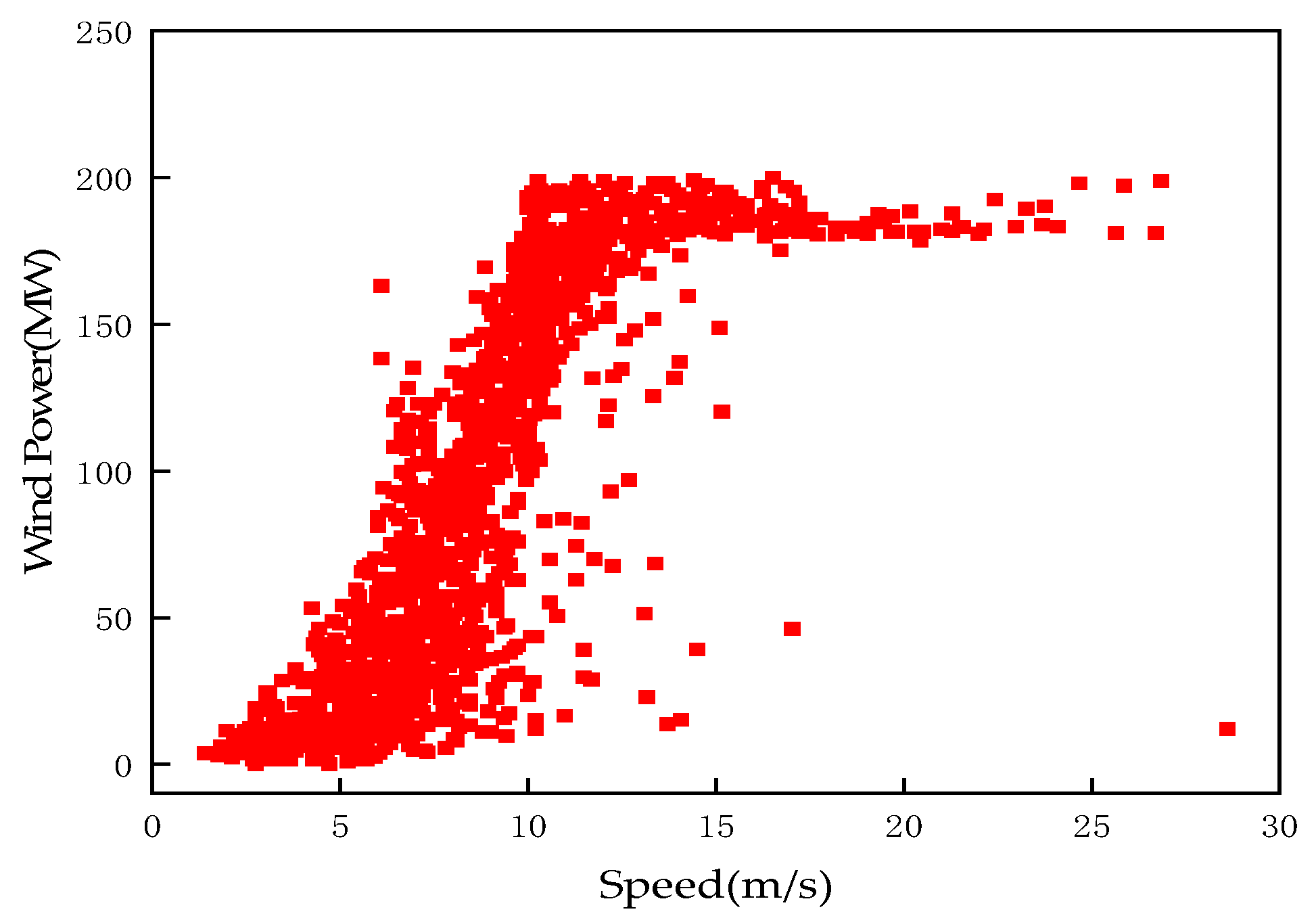
Figure 1. Scatterplot of wind speed–wind power.
Energies 16 05476 g001
Figure 2. Box block diagram.
Energies 16 05476 g002
Figure 3. LSTM network basic unit.
Energies 16 05476 g003
Figure 4. BiLSTM network structure.
Energies 16 05476 g004
Figure 5. Predictive model flow.
Energies 16 05476 g005
Figure 6. Wind farm wind power situation: (a) March wind power data; (b) June wind power data; (c) September wind power data; (d) December wind power data.
Energies 16 05476 g006
Figure 7. Sliding window prediction schematic.
Energies 16 05476 g007
Figure 8. Data normalization results.
Energies 16 05476 g008
Figure 9. GRA chart.
Energies 16 05476 g009
Figure 10. Wind power data decomposition results.
Energies 16 05476 g010
Figure 11. Sample entropy reconstruction component map.
Energies 16 05476 g011
Figure 12. BiLSTM network training results: (a) reconstructing component F1, (b) reconstructing component F2, (c) reconstructing component F3, (d) reconstructing component F4, and (e) reconstructing component F5.
Energies 16 05476 g012
Figure 13. Comparison of wind power forecasts: (a) March forecast comparison, (b) June forecast comparison, (c) September forecast comparison, and (d) December forecast comparison.
Energies 16 05476 g013aEnergies 16 05476 g013b
Table 1. Statistical summary of weather information.
VariablesUnitMaximumMinimumMeanStandard Deviation
PowerMW0.258202.22953.90856.733
Speedm/s021.0565.3473.836
Direction°0360158.63989.834
Temperature°C−18.66240.13111.32514.027
PressurehPa874.584905.307888.5095.793
Humidity%2.50694.92133.59320.761
Table 2. Statistical information on wind power.
MonthsMaximumMinimumMEANKurtosisSkewness
March201.2530.43460.005−0.6120.855
June170.5780.40251.105−0.9440.619
September189.8380.32252.589−0.9600.676
December201.6300.36850.678−0.3980.935
Table 3. Sample entropy values of the raw wind power components.
ComponentSE Value
IMF11.286
IMF20.986
IMF30.864
IMF40.786
IMF50.507
IMF60.464
IMF70.257
IMF80.243
IMF90.229
IMF100.136
IMF110.114
IMF120.107
Table 4. Correspondence between reconstructed power components and original power components.
Reconstructing ComponentComponent
F1IMF1
F2IMF2 + IMF3 + IMF4
F3IMF5 + IMF6
F4IMF7 + IMF8 + IMF9
F5IMF10 + IMF11 + IMF12
Table 5. The deterministic forecasting performances of the models with different decomposition algorithms.
Data SetModelRMSEMAEMAPERAR
MarchCEEMDAN-SE-BiLSTM-MC1.7921.4790.2020.999
CEEMDAN-SE-BiLSTM5.0814.2160.4620.993
CEEMDAN-BiLSTM6.2525.7510.2390.990
BiLSTM10.7429.6670.5960.971
LSTM16.01112.030.8130.937
JuneCEEMDAN-SE-BiLSTM-MC3.7242.8260.4310.953
CEEMDAN-SE-BiLSTM4.3593.1920.5580.922
CEEMDAN-BiLSTM4.5593.3410.6660.915
BiLSTM4.7194.4160.8030.909
LSTM5.6665.1070.9530.868
SeptemberCEEMDAN-SE-BiLSTM-MC1.4761.2750.4190.999
CEEMDAN-SE-BiLSTM5.5963.4670.5200.985
CEEMDAN-BiLSTM6.3744.4560.5420.980
BiLSTM6.7784.8410.5750.978
LSTM7.0745.1650.8600.976
DecemberCEEMDAN-SE-BiLSTM-MC1.4291.0150.1130.997
CEEMDAN-SE-BiLSTM2.1511.2150.2330.993
CEEMDAN-BiLSTM4.8553.7460.4230.969
BiLSTM5.5164.1890.4540.960
LSTM8.5036.1650.4560.905
Disclaimer/Publisher’s Note: The statements, opinions and data contained in all publications are solely those of the individual author(s) and contributor(s) and not of MDPI and/or the editor(s). MDPI and/or the editor(s) disclaim responsibility for any injury to people or property resulting from any ideas, methods, instructions or products referred to in the content.