Article

Advanced Machine Learning Techniques for Accurate Very-Short-Term Wind Power Forecasting in Wind Energy Systems Using Historical Data Analysis

by
G. Ponkumar
1,*,
S. Jayaprakash
1 and
Karthick Kanagarathinam
2
1
School of Electrical and Electronics Engineering, Sathyabama Institute of Science & Technology, Chennai 600 119, Tamil Nadu, India
2
Department of Electrical and Electronics Engineering, GMR Institute of Technology, Rajam 532 127, Andhra Pradesh, India
*
Author to whom correspondence should be addressed.
Energies 2023, 16(14), 5459; https://doi.org/10.3390/en16145459
Submission received: 19 June 2023 / Revised: 10 July 2023 / Accepted: 15 July 2023 / Published: 18 July 2023
(This article belongs to the Section A3: Wind, Wave and Tidal Energy)

Abstract

:
Accurate wind power forecasting plays a crucial role in the planning of unit commitments, maintenance scheduling, and maximizing profits for power traders. Uncertainty and changes in wind speeds pose challenges to the integration of wind power into the power system. Therefore, the reliable prediction of wind power output is a complex task with significant implications for the efficient operation of electricity grids. Developing effective and precise wind power prediction systems is essential for the cost-efficient operation and maintenance of modern wind turbines. This article focuses on the development of a very-short-term forecasting model using machine learning algorithms. The forecasting model is evaluated using LightGBM, random forest, CatBoost, and XGBoost machine learning algorithms with 16 selected parameters from the wind energy system. The performance of the machine learning-based wind energy forecasting is assessed using metrics such as mean absolute error (MAE), mean-squared error (MSE), root-mean-squared error (RMSE), and R-squared. The results indicate that the random forest algorithm performs well during training, while the CatBoost algorithm demonstrates superior performance, with an RMSE of 13.84 for the test set, as determined by 10-fold cross-validation.

1. Introduction

Wind power has gained prominence as an important renewable energy source in recent years due to its abundance of advantages, including carbon-free output and the absence of harmful gas emissions [1]. The depletion of reserves and increased demand for fossil fuels have severe effects on the ecosystem. Therefore, the public authority is taking the required measures to encourage the use of renewable energy sources as a replacement for fossil fuels. Even if fossil fuels’ percentage of primary energy consumption has dropped to below 75%, carbon dioxide emissions from power stations are expected to rise by 20% by 2040 [2]. The result of this is expected to be a 3.6 °C rise in the average global temperature over the long run.
There are two possible ways to harvest wind energy, and they are known as onshore and offshore wind [3]. When comparing wind and solar power, it is important to keep in mind that solar power can only be produced during the day, while wind power can be generated 24/7, meaning it is available throughout the day and night. It is anticipated that the cost, handling, transit, and production costs of energy generated from wind will be more stable than those of power derived from fossil fuels. The costs of wind energy are expected to be more consistent and less susceptible to fluctuations compared to fossil fuel-based power.
Wind is generated when pressure and thermal differentials around the planet respond to the sun’s heat. When air heated by the sun rises and colder air sinks, this creates a circulation pattern on a global scale. It is reported that the wind converts just around 2% of the solar energy that the Earth receives into kinetic energy [4]. Wind energy systems use wind turbines and generators to transform the kinetic energy of the wind into electricity. Wings mounted to a hub revolve in accordance with the aerodynamic force exerted by the wind to accomplish this. The electricity people use every day comes from the generator that is generated by this motion [5]. Not everywhere has the right conditions for wind turbines to be a practical source of electricity production. A site’s wind power potential is evaluated by collecting a time series of raw wind data records, including wind speed, wind direction, temperature, and air pressure, before a wind turbine is installed onsite [6].
Figure 1 displays a steady rise in global installed wind power capacity [7], which reached 824,874 MW in 2021. The Indian numbering system has been followed to represent the installed power capacity.

1.1. Need for Wind Energy Forecasting

Power from the wind is forecasted in terms of how much electricity one or more wind turbines (together called a wind farm) are likely to generate within the next few months to a year. Power output potential during a given time period is often forecast in regard to the available energy of the wind farm. The forecasting is required to maintain a constant equilibrium among both electricity use and generation that will prevent power quality problems [8]. Since wind power generation is intermittent, it is necessary to have backup generators on hand in case of outages. A coal plant takes six hours to start up, while a nuclear power plant takes twelve hours [9]. Once wind power contributes more than a low amount to the grid’s total electrical output, the issue becomes more convoluted. With more accurate predictions, utilities can use fewer spinning reserves, which are often powered by natural gas, to meet electricity demand.
Theoretically, wind power delivered by the rotor of the wind turbine [10] is given by
P r = 0.5   ρ π   R 2 C p ( λ ,   β ) v 3
where ρ —air density;
R—the radius of the rotor;
v—Wind speed;
C p —the coefficient of rotor power;
λ —blade pitch angle;
β —tip speed ratio.

1.2. Classification of Wind Energy Prediction

Wind power generation forecasting can be examined at a variety of time scales, based on the context [11]. Very-short-term forecasting involves estimating wind energy production with a time horizon of seconds to minutes. In the context of controlling turbines and managing electrical grids in real time, this is an essential tool. For dispatch planning and smart load-shedding procedures, it is necessary to have access to short-term forecasts, which will include predictions of wind power generation from 30 min up to hours. Decisions about whether or not to turn the turbine on or off, whether for reasons of safety or market conditions, will be guided by medium-term forecasting that extends from six hours to one day. The purpose of long-term forecasting is to plan maintenance or unit commitment and optimize operating costs over the course of several months or perhaps a year [12].

1.3. Forecasting Methods

The forecasting of wind is evaluated from the predictable power production of the wind turbines. This power production is articulated in kW or MW depending on the insignificant capacity of the wind farm. The wind power forecasting tools available today are based on mix of physical and statistical methods. The data that are required for wind forecasting are composed from several turbines at wind farm. Wind forecasting usually differs from place to place. This may not allow for a unique forecasting procedure to be developed for adoption at all the probable sites. Wind forecasting may be classified into four types based on time scales. Wind power forecasting can be viewed in terms of the various approaches as physical and statistical.
Physical approach: The physical approach takes into account restrictions based on a comprehensive physical description of the wind flow inside as well as around the wind farm. It is derived from numerical weather prediction (NWP) using weather forecast data [13] like atmospheric variables (temperature, pressure, etc.), and also the characteristics of wind farm area, such as farm layout, roughness, obstacles, and other secondary data. These data are utilized to forecast wind power by taking into account the wind speed and converting it into power generated by wind turbines at the wind farm.
Statistical approach: Statistical approaches are based on preparation with historical data and output generation through statistical models without taking physical observable fact into account [14]. Artificial neural networks, fuzzy logic, regression trees, and support vector machines are some of the statistical methodologies that are now being used. Statistical approaches yield a good result of wind forecasting.
This article presents a machine learning-based model for making very-short-term predictions based on the values of 11 features chosen from the wind energy conversion system’s historical data. The features of the historical data have the information of the weather, turbine, and rotor. The wind power is the direct prediction parameter in this model. The sampling rate of the dataset is 10 min.
In addition, we also present the wind rose diagram for wind speed analysis. We performed exploratory data analysis to know the insights of the adopted dataset.

2. Related Work

Ying-Yi Hong et al. proposed a hybrid deep learning neural network that is capable of forecasting wind power generation up to twenty-four hours in advance [15]. This approach makes use of a convolutional neural network (CNN), which is then followed by a radial basis function neural network (RBFNN), which has a double Gaussian function (DGF) as its activation function. By combining convolution, kernel, and pooling processes, the CNN is able to extract wind power characteristics. Using a DGF, supervised RBFNN handles ambiguous features. Generations of wind power were modelled using data collected from a real wind farm. There are 4 times a year where the results have r-squared values (a measure of reliability) above 0.88. Using time-series data of 10 min, C. Gallego et al. [16] undertook an investigation that focused exclusively on one-step-ahead prediction. They forecasted using the time-series autoregressive (AR) model, conditional parametric autoregressive models (CPARX) and threshold autoregressive open-loop (TARSO) models. They found that the normalized root-mean-square error (NRMSE) ranged from 3.91 to 5.82 for CPARX (wind direction, wind speed) model.
Bri-Mathias Hodge et al. [17] studied the effectiveness of statistical time-series analytic methods, namely autoregressive integrative moving average (ARIMA) models, in predicting the future wind energy production from historical records.
Artificial neural network (ANN) models were constructed by Amila et al. [18] in order to forecast the amount of power that will be generated by the wind at “Pawan Danawi”, which is an operational wind farm situated in Sri Lanka. The amount of power created by the wind was utilized as the dependent variable in the artificial neural network models that were constructed, while the wind speed, wind direction, and the temperature of the surrounding environment were employed as independent variable matrices in the models. In order to evaluate the accuracy of the models that were produced by them, the learning techniques of Levenberg–Marquardt (LM), scaled conjugate gradient (SCG), and Bayesian regularization (BR) were utilized. In addition, the model was calibrated for five different validation percentages, ranging from 5% to 25% in 5% increments, for each algorithm, in order to determine which training method yielded the best results and which percentages of training and validation were the most appropriate. Mean-squared error (MSE), coefficient of correlation, root-mean-squared error ratio, Nash number, and BIAS were the metrics that were utilized in the process of analysing how well the ANN models that were constructed performed.
Upma Singh and M. Rizwan [19] developed machine learning-based models that are capable of accurately estimating the amount of power generated by wind. The results of the experiments indicate that a gradient boosting regression model performs better than other benchmark models when it comes to the accuracy of its forecasts.
Anomalies in wind power generation can have implications for the stability and integration of wind energy into the power grid. By detecting and understanding anomalies in wind data, grid operators can better manage the variability and uncertainty of wind power, leading to improved grid stability and more effective integration of renewable energy sources [20]. Table 1 provides an overview of various wind power prediction models and their evaluations.

3. Materials and Methods

Figure 2 shows the block diagram of the proposed approach. The first stage is data preprocessing, which removes duplicate and missing value instances. The second stage is attribute selection and exploratory data analysis. The third stage is ML model development and performance analysis.

3.1. Data

The wind power dataset is available in Kaggle’s public domain. It can be accessed through this link [31]. It consists of a variety of weather, generator, and rotor components. During January of 2018, and continuing through March of 2020, data were collected. Readings were recorded every ten minutes at regular intervals. Table 2 shows the descriptive statistics summary of the raw dataset. The raw dataset is composed of a maximum of 94,750 instances and 21 features, including the date and time attributes. The index shows the various features that were available in the dataset. The count, mean, standard deviation, percentiles, and min–max values of all the features can be found in Table 2. The dataset includes various features that provide information about the wind turbine system. The ‘Ambient Temperature’ feature represents the temperature of the surrounding environment and is usually measured in degrees Celsius (°C). ‘Bearing Shaft Temperature’ indicates the temperature of the bearing shaft and is typically measured in degrees Celsius (°C). ‘Blade 1 Pitch Angle’ denotes the pitch angle of the first blade of the wind turbine and is measured in degrees. Similarly, ‘Blade 2 Pitch Angle’ represents the pitch angle of the second blade and ‘Blade 3 Pitch Angle’ signifies the pitch angle of the third blade, both measured in degrees. ‘Control Box Temperature’ refers to the temperature of the control box and is typically measured in degrees Celsius (°C). ‘Gearbox Bearing Temperature’ indicates the temperature of the gearbox bearings, measured in degrees Celsius (°C). The ‘Gearbox Oil Temperature’ represents the temperature of the gearbox oil and is also measured in degrees Celsius (°C).
‘Generator RPM’ denotes the rotational speed of the generator and is measured in revolutions per minute (RPM). ‘Generator Winding 1′ and ‘Generator Winding 2′ represent the temperature of the two windings and are typically measured in degrees Celsius (°C). ‘Hub Temperature’ refers to the temperature of the hub of the wind turbine, usually measured in degrees Celsius (°C). ‘Main Box Temperature’ represents the temperature of the main box and is typically measured in degrees Celsius (°C). ‘Nacelle Position’ indicates the position of the nacelle, which is the housing structure on top of the wind turbine tower. It does not have a specific unit of measurement.
Furthermore, ‘Reactive Power’ denotes the power that oscillates back and forth between the source and load due to reactive components in the system. It is usually measured in kilovolt-ampere reactive (kVAR). ‘Rotor RPM’ represents the rotational speed of the rotor and is measured in revolutions per minute (rps). ‘Turbine Status’ indicates the status or condition of the wind turbine and does not have a specific unit of measurement. ‘Wind Direction’ refers to the direction from which the wind is blowing and is typically measured in degrees. ‘Wind Speed’ signifies the speed of the wind and is usually measured in meters per second (m/s). Finally, ‘Active Power’ represents the actual power output of the wind turbine and is usually measured in kilowatts (kW). In this model, ‘ActivePower’ serves as the target variable.

3.2. Preprocessing

During data processing, missing numbers are almost often the result of human error or an error in the system caused by a malfunction in the equipment being used. The problem of missing numbers is widespread in all fields that deal with data, and creates a variety of concerns, such as a decline in performance, problems with data analysis, and skewed conclusions [32]. It is seen in descriptive statistics that there are missing or null values. The average value of the ‘ControlBoxTemperature’ attribute is 0. It was decided to remove the ‘ControlBoxTemperature’ feature. In addition, the dataset’s missing, null, and duplicate instances were eliminated. During this stage, various data cleaning steps were performed to ensure the quality and integrity of the dataset. One crucial step was the removal of duplicate instances, which helps eliminate redundant or identical data points. This process involves identifying and removing instances that have identical values across all attributes. After removing the duplicate instances, the dataset had 32,818 instances with 20 attributes, including the date and time feature. This process helps prevent bias and ensures that each instance contributes unique information to the analysis. The data type conversion of the ‘date’ attribute from object to date and time was performed.

3.3. Attribute Selection

A data visualization tool known as a heat map (sometimes spelled heatmap) illustrates the magnitude of a phenomenon by colouring it in two dimensions. The reader will receive clear visual clues about how the phenomenon is clustered or fluctuates across space depending on whether the variation in colour is by hue or intensity. Using the heat map, we were able to find features that are not relevant. By performing feature selection, one creates a feature subset from the original features by deleting features that are unnecessary or redundant [33]. A positive correlation implies a strong dependency, whereas a negative correlation shows a significant inverse dependency; a correlation coefficient near zero indicates a weak dependency [34]. Figure 3 shows the heat map of the wind power dataset.
The features ‘GeneratorWinding1Temperature’, ‘GeneratorWinding2Temperature’, and ‘WindSpeed’ exhibit a strong correlation with a coefficient value of 0.93, indicating a significant association between these temperature variables, wind speed, and the generated wind power. The efficiency and performance of the generator can be influenced by temperature changes. When generators convert mechanical energy into electrical energy, some of the input energy is lost as heat due to resistance in the generator windings and other components. Higher temperatures can intensify these thermal losses, resulting in a decrease in overall efficiency. Additionally, temperature fluctuations impact the electrical resistance of the generator windings. Generally, higher temperatures cause an increase in electrical resistance, leading to higher losses and reduced electrical output. Increased resistance can also lead to voltage drops and inefficient power transmission. The two attributes ‘TurbineStatus’ and ‘AmbientTemperatue’ have weak dependency with Active Power. These two features were removed from the prediction model development. Now, the number of features that are considered for model development becomes 17, excluding the ‘Date’ feature.

3.4. Outlier Removal

If a measurement is positioned at an abnormal distance from all other values in a random sample collected from a population, then that observation is regarded to be an outlier. It has the potential to significantly influence the findings of any hypothesis tests and statistical examinations that users perform. Hence, the outliers of the various attributes need to be deleted since they are indicative of measurement issues, problems in data entry or processing, or inadequate sampling [35]. Now, after the removal of outliers in the preprocessed dataset, the total number of instances becomes 31503. This is the final number of instances used for the exploratory data analysis and machine learning regression model development. The number of features used in the model’s development is 16. They are ‘BearingShaftTemperature’, ‘Blade1PitchAngle’, ‘Blade2PitchAngle’, ‘Blade3PitchAngle’, ‘GearboxBearingTemperature’, ‘GearboxOilTemperature’, ‘GeneratorRPM’, ‘GeneratorWinding1Temperature’, ‘GeneratorWinding2Temperature’, ‘HubTemperature’, ‘MainBoxTemperature’, ‘NacellePosition’, ‘ReactivePower’, ‘RotorRPM’, ‘WindDirection’, and ‘WindSpeed’. The ‘ActivePower’ attribute is the dependent or target variable. Data are considered to be normal if their skewness is in the range of −2 to +2 and their kurtosis is within in the range of −7 to +7, as stated by Hair et al. [36] and Bryne [37].
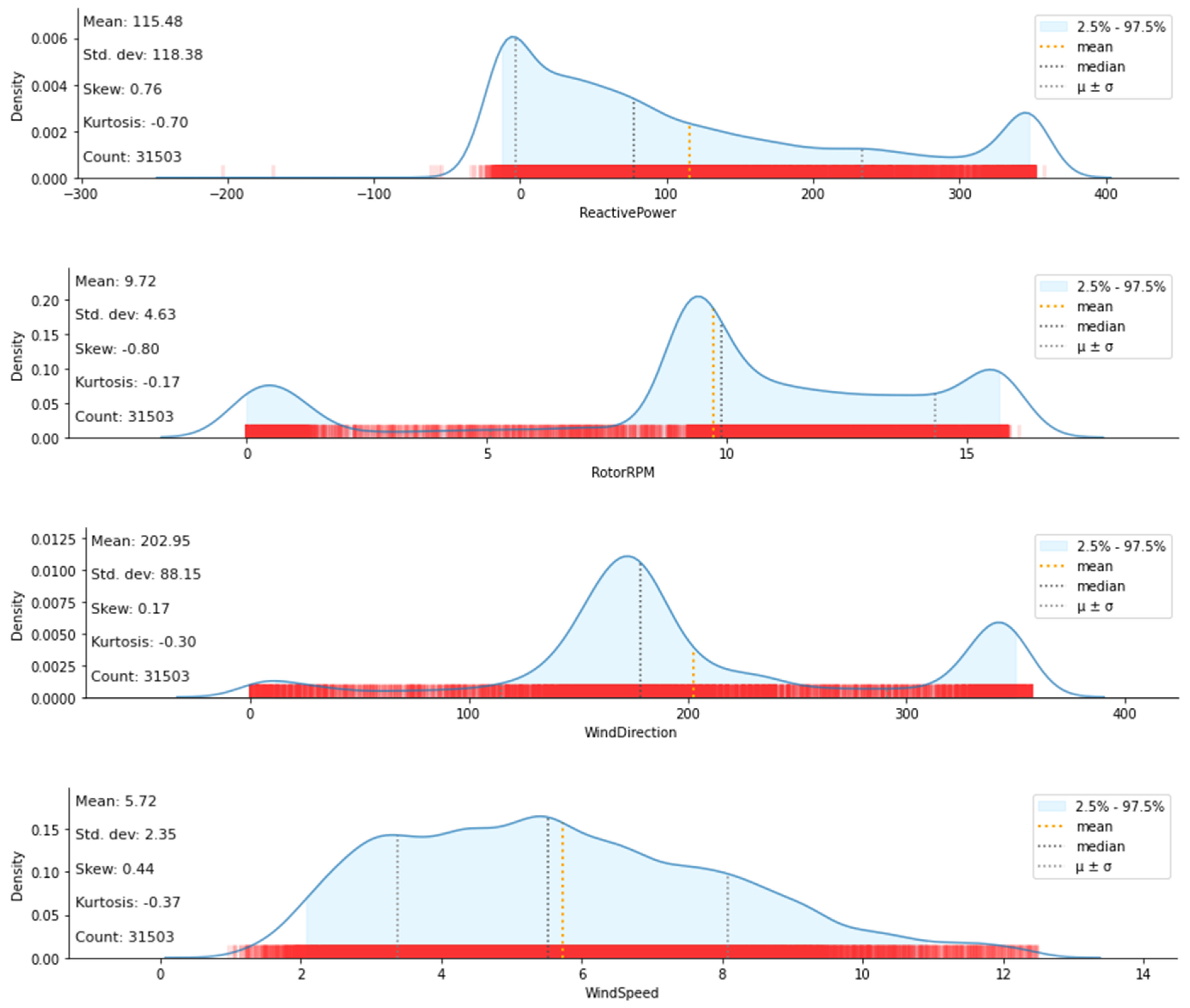
Figure 4 illustrates the distribution of dataset features, skewness, and kurtosis values after outlier removal. The x-axis of the figure represents the names of the features, and the figure displays the mean, standard deviation, skewness, kurtosis, and the count of instances for each individual feature. The range from 2.5% to 97.5% represents the central 95% of the distribution. It is commonly referred to as the “95% confidence interval” or the “interquartile range” (IQR). This range captures the majority of the data points, excluding the extreme values. It provides a measure of the typical or average range of values within the dataset, while omitting outliers or extreme values that may skew the distribution.

3.5. Exploratory Data Analysis

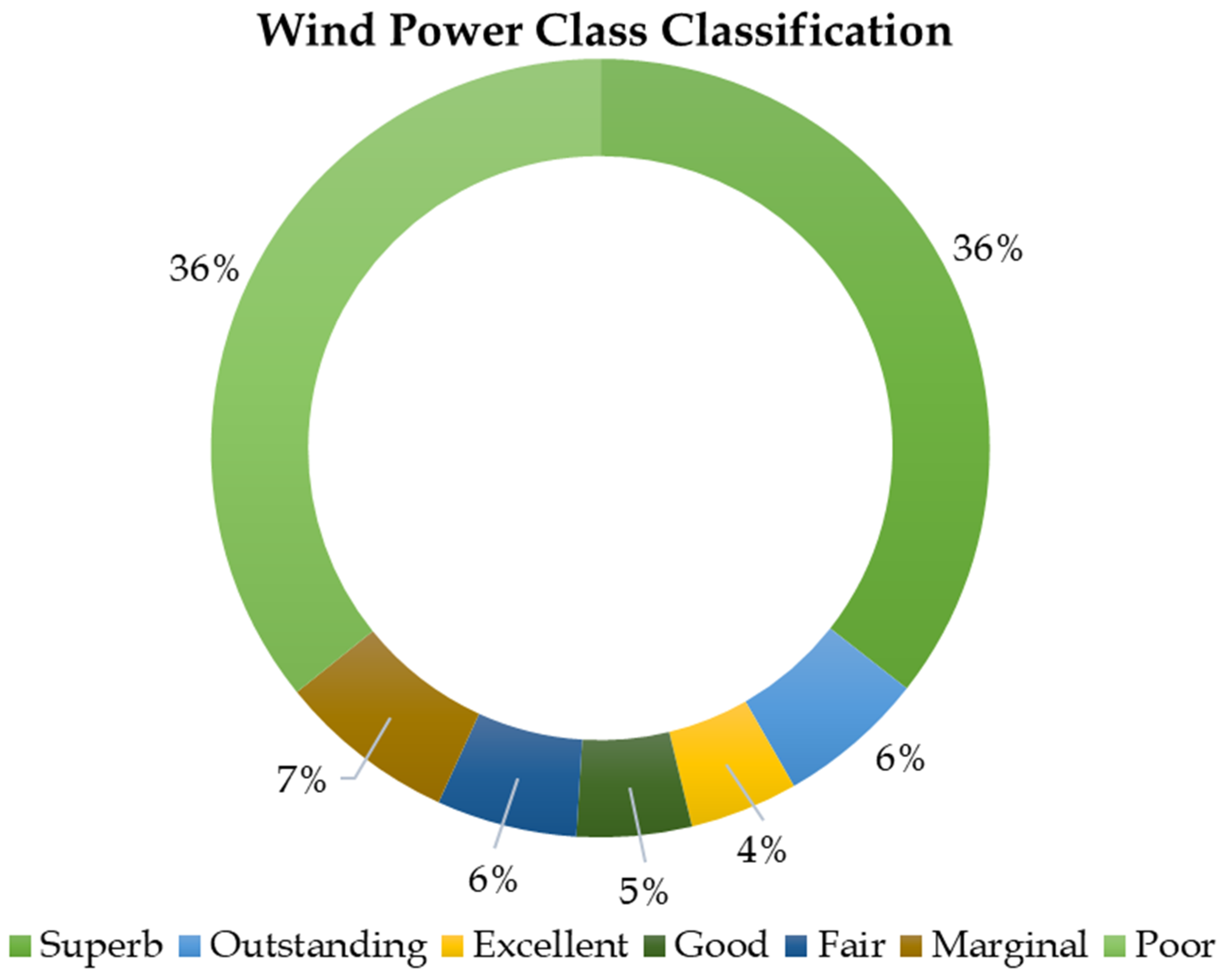
Exploratory data analysis, abbreviated as EDA, is a technique that examines and investigates datasets in order to summarize their primary attributes. This technique frequently makes use of data visualization approaches. In this section, we examined the processed dataset and extracted data insights. Table 3 shows the wind power category extracted from M. Irwanto et al. [38]. Figure 5 shows the data distribution of the wind power dataset based on the wind power category shown in Table 3. It is observed that 36% of the wind power falls into the superb and outstanding categories. The dataset has the information from January 2018 until March 2020. It was found that the site is located in the good region.

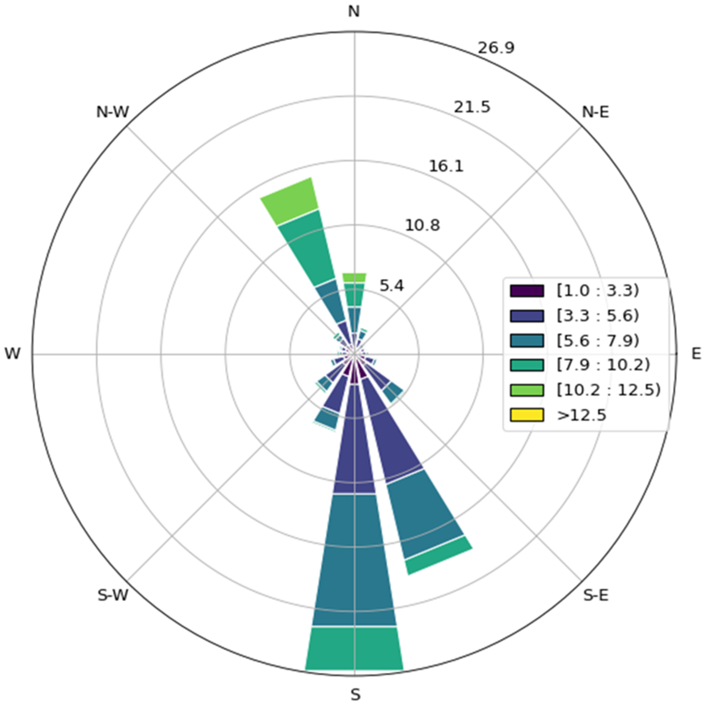
3.5.1. Wind Rose Analysis

The wind rose analysis is carried out to determine the dominant wind direction. Figure 6 shows the wind rose diagram of the wind power dataset. The wind rose diagram illustrates the overall wind direction and speed for each period of sampling. The wind rose is presented in a circular shape, which indicates the direction from which the winds moved, and the length of each “spoke” around the circle indicates the frequency with which the wind flew from that particular direction. It was observed that the frequent wind flow is in the direction of south.

3.5.2. Dataset Insights

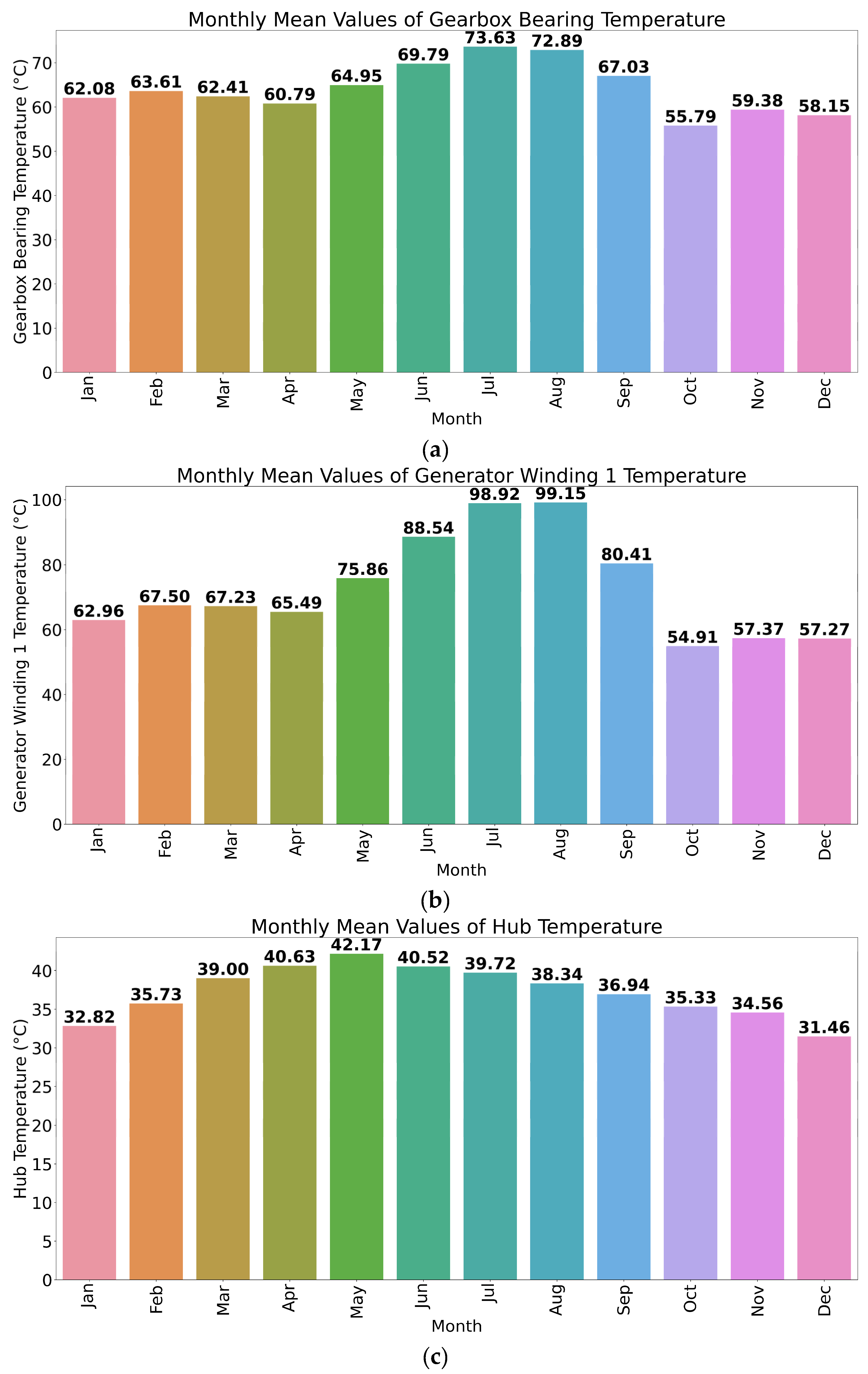
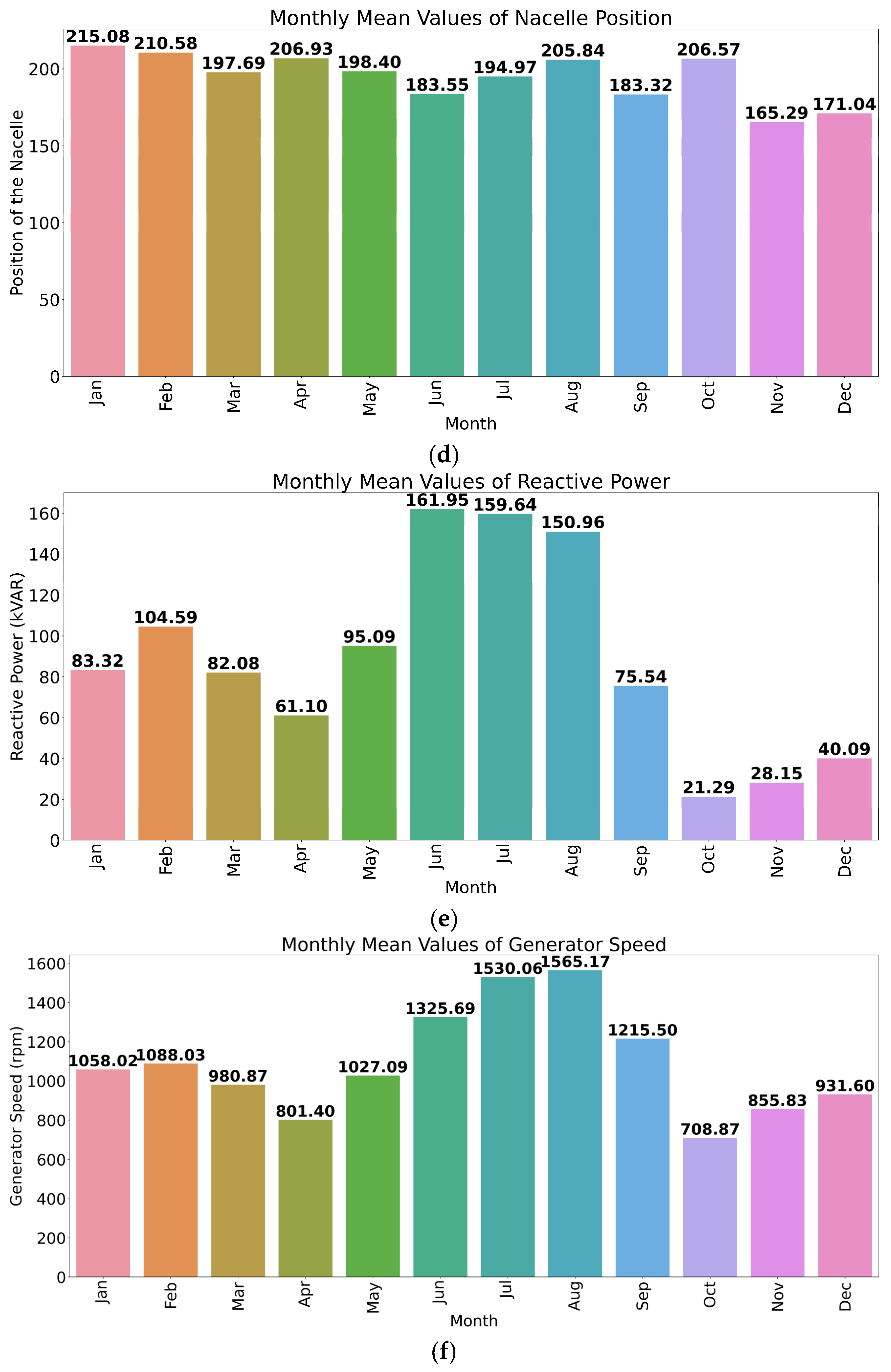
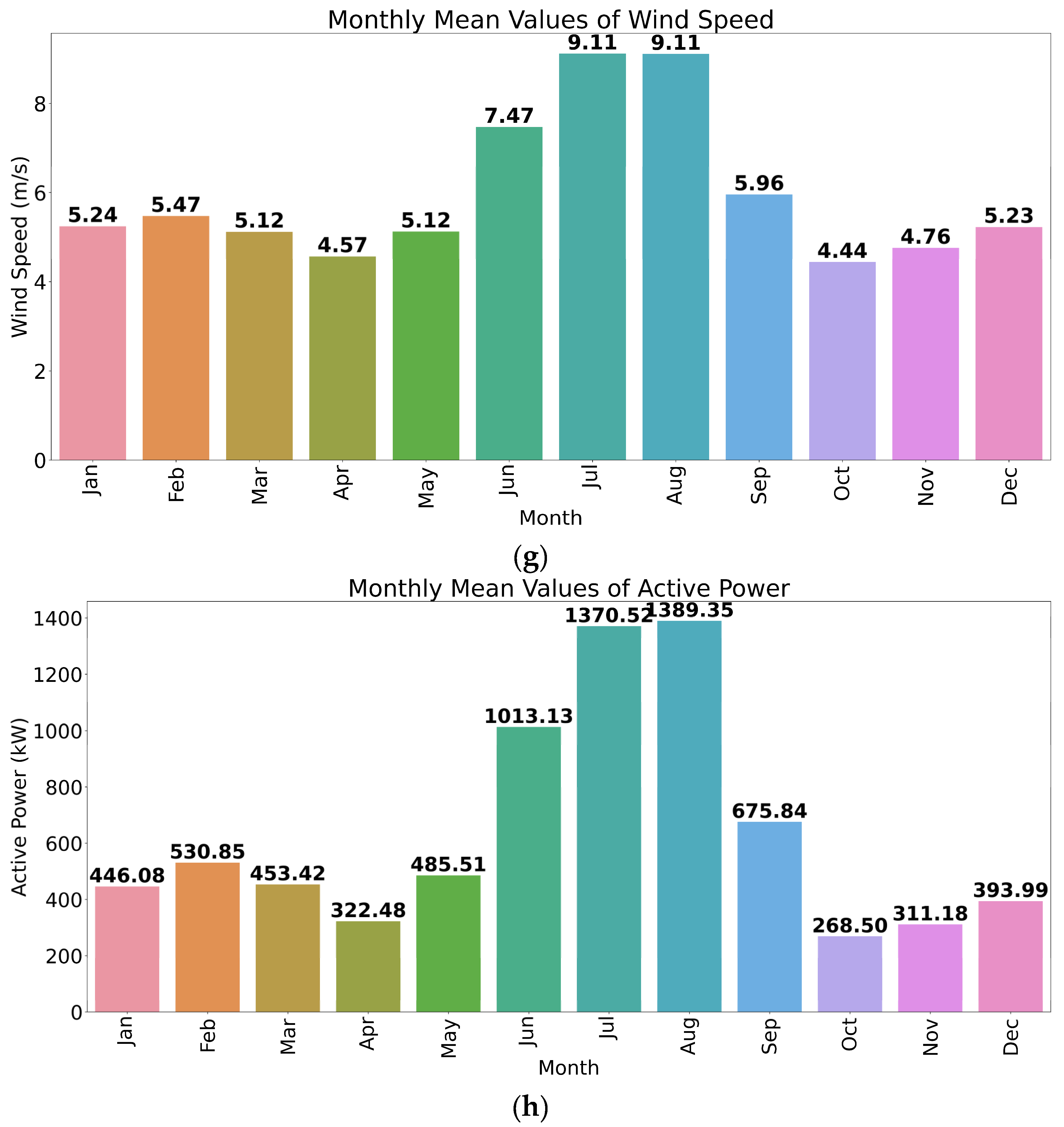
Figure 7 illustrates the mean values of various parameters based on the month, including (a) Gearbox Bearing Temperature, (b) Generator Winding1 Temperature, (c) Hub Temperature, (d) Nacelle Position, (e) Reactive Power, (f) Generator RPM, (g) Wind Speed, and (h) Active Power. The gearbox plays a crucial role in increasing the rotational speed from the wind turbine’s low-speed drive shaft to the high-speed shaft, which is connected to an electrical generator.
The analysis of the dataset reveals that the wind power generation reaches its peak during the months of July and August. Conversely, the wind power generation is relatively lower in October. Figure 8 presents the daily mean values of wind speed, further highlighting this observation. Due to the large dataset, a random sample of 10,000 data points was considered for plotting purposes, while the summary statistics are calculated based on the entire dataset. It is evident from Figure 8 that the highest wind speeds occur in July and August.

3.6. Machine Learning Algorithms

The regression model was created using four machine learning algorithms. They are LightGBM, random forest, CatBoost, and XGBoost.

3.6.1. LightGBM

The library known as LightGBM, which stands for “Light Gradient Boosted Machine”, was developed at Microsoft and offers a productive implementation of the gradient boosting technique. The most significant advantage provided by the LightGBM is the modification of the training algorithm, which not only makes the process considerably quicker but also, in many instances, produces a more accurate model [39]. The LightGBM method takes as input a supervised training set X and a loss function L(y, f(x)) whose anticipated value is to be minimized f ^ (x). It is given in Equation (2).
f ^ = arg m i n f   E y ,   X   L   ( y ,   f ( x ) )

3.6.2. Random Forest

The formation of random forests [35] for the purpose of regression involves developing trees in dependence on a random vector Θ in such a manner that the tree predictor h (x, Θ) takes on numeric values rather than class labels. The outputted values are presented in numerical form, and the training set was chosen arbitrarily from the random vector Y, X distribution [40]. The random forest predictor was constructed by calculating the mean value across all k of the trees {h (x, Θk)}. It is represented in Equation (3).
Random   forest   prediction = 1 K k = 1 K h k ( x )

3.6.3. CatBoost

Yandex’s CatBoost method is an efficient implementation of the gradient boosting technique. The support for categorical input variables is the key advantage offered by the CatBoost algorithm. CatBoost, which stands for “Category Gradient Boosting”, is the name given to this library as a result of this [41]. Equation (4) is used by CatBoost to define the encoded value, x ^ k i for the ith categorical value during Decision Tree h t + 1 fitting; rather than strictly following it, it employs a variant of it in its assessment.
x ^ k i = x j D k 𝟙   x j i = x k i · y j + a p x j D k 𝟙   x j i = x k i + a  

3.6.4. XGBoost

Extreme gradient boosting [42], which can be abbreviated to XGBoost, is the name of a library that offers a practical and effective implementation of the gradient boosting technique. The direct application of XGBoost for predictive modelling in the form of regression is possible.
Using the universal function, we may obtain the estimated model, as shown in the following formula:
y ^ i t = k = 1 t f k ( x i ) = y ^ i ( t 1 ) + f t ( x i )
where
y ^ i t = forecasts at the stage t
f t ( x i ) = a learner at stage t
x i = the input variable
y ^ i ( t 1 ) = forecasts at the stage t − 1

3.7. Results and Discussion

The total number of instances to develop the prediction model is 31,503. The number of features used in the model’s development is 16. The training and test set is split into an 80:20 ratio. The training phase consists of 25,202 instances and test phase consists of 6301 instances. The model’s performance is evaluated using 10-fold cross validation. The process of testing machine learning models by using a subset of the available data includes the usage of a resampling approach that is known as cross-validation. The procedure has one parameter, which is represented by the letter k, and it is used to specify the number of distinct groups by which a particular dataset is to be divided. Because of this, the process is commonly referred to as k-fold cross-validation. We employed 10-fold cross validation to assess the performance. This helps us to avoid the overfitting issue in the prediction model. Data were recorded from January 2018 until March 2020. Readings were recorded at a 10 min intervals. So, the prediction model helps us to predict the short-term wind power generation.

3.7.1. Hyperparameter Optimization

In most cases, a hyperparameter will have a predictable effect on a model in the broad sense; nevertheless, it is not always obvious how to optimally configure a hyperparameter for a particular dataset. In addition, the majority of machine learning models consist of a wide variety of hyperparameters, some of which may interact with one another in a nonlinear fashion.
As a consequence of this, it is frequently necessary to look for a collection of hyperparameters that bring about the greatest performance of a model when applied to a dataset. This is referred to as hyperparameter search, or hyperparameter optimization. We used random search as the method for optimizing the hyperparameters. It carries this out by defining a search space as a domain of hyperparameter values that is bounded on all sides and then randomly sampling points from inside that domain.

3.7.2. Prediction Model’s Performance

The performance of a regression model was assessed using mean absolute error (MAE), mean-squared Error (MSE), root-mean-squared error (RMSE) and R-squared value.
The MAE is determined using Equation (6).
M A E = | ( y i y p ) | n
The MSE is determined using Equation (7).
M S E = ( y i y p ) 2 n
The RMSE is determined using Equation (8).
R M S E = ( y i y p ) 2 n
Here, y i and y p are the actual and predicted values for ‘n’ number of instances.
R-Squared (R2) or coefficient of determination is calculated by Equation (9).
R 2 = 1 ( y i y p ) 2 ( y i y i ¯ ) 2  
Here, y i ¯ is the mean of all the actual values.
Table 4 presents the performance metrics for each model on both the training set and test set. The results show that all models perform well, with high R2 values close to 1, indicating a strong correlation between the predicted and actual values. The models achieve relatively low MAE, MSE, and RMSE, indicating small errors in the prediction of wind power. The random forest model exhibits the lowest MAE, MSE, and RMSE values on the training set, suggesting superior performance in capturing the training data patterns. However, the CatBoost model demonstrates the lowest RMSE on the test set, indicating better generalization ability.
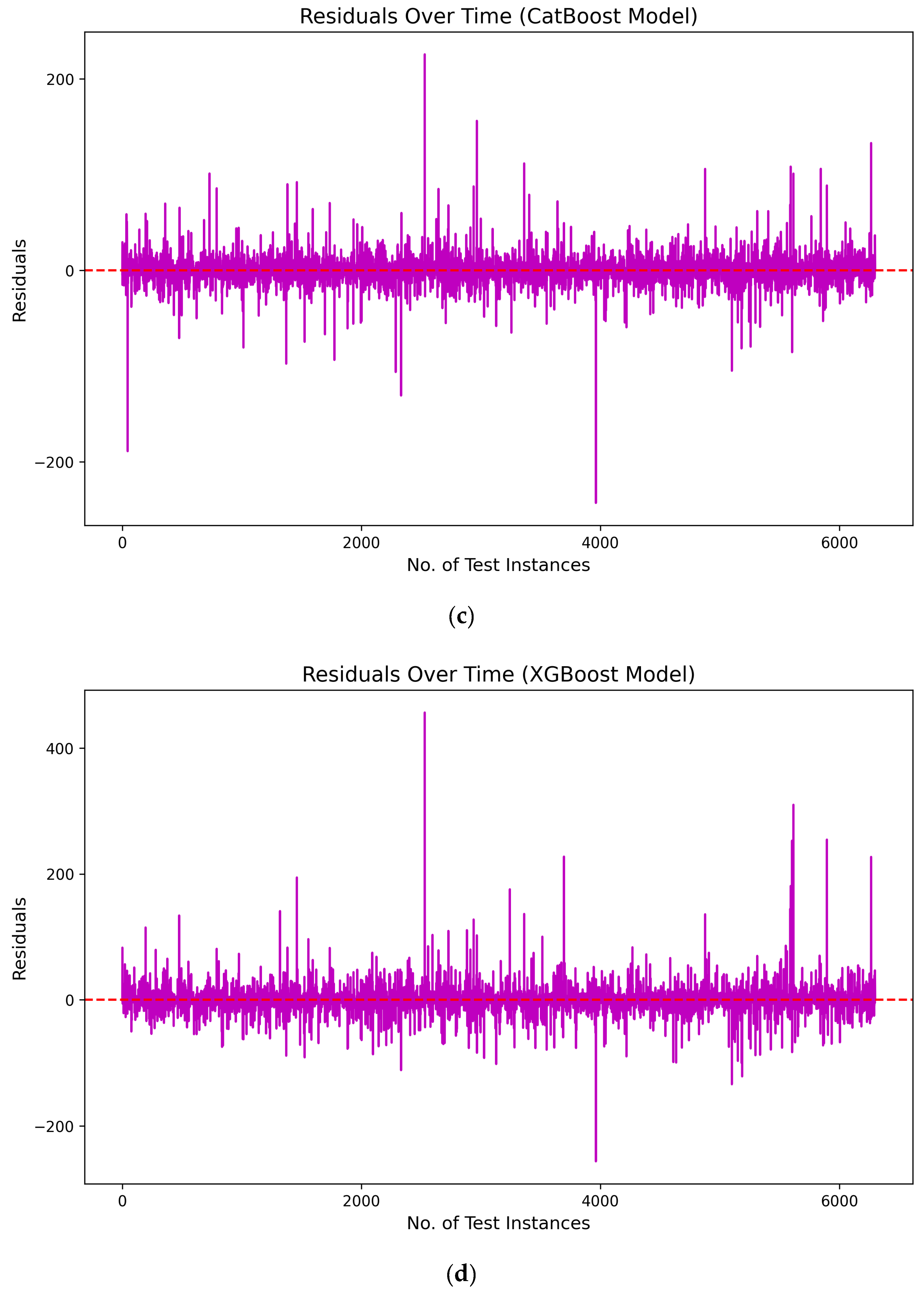
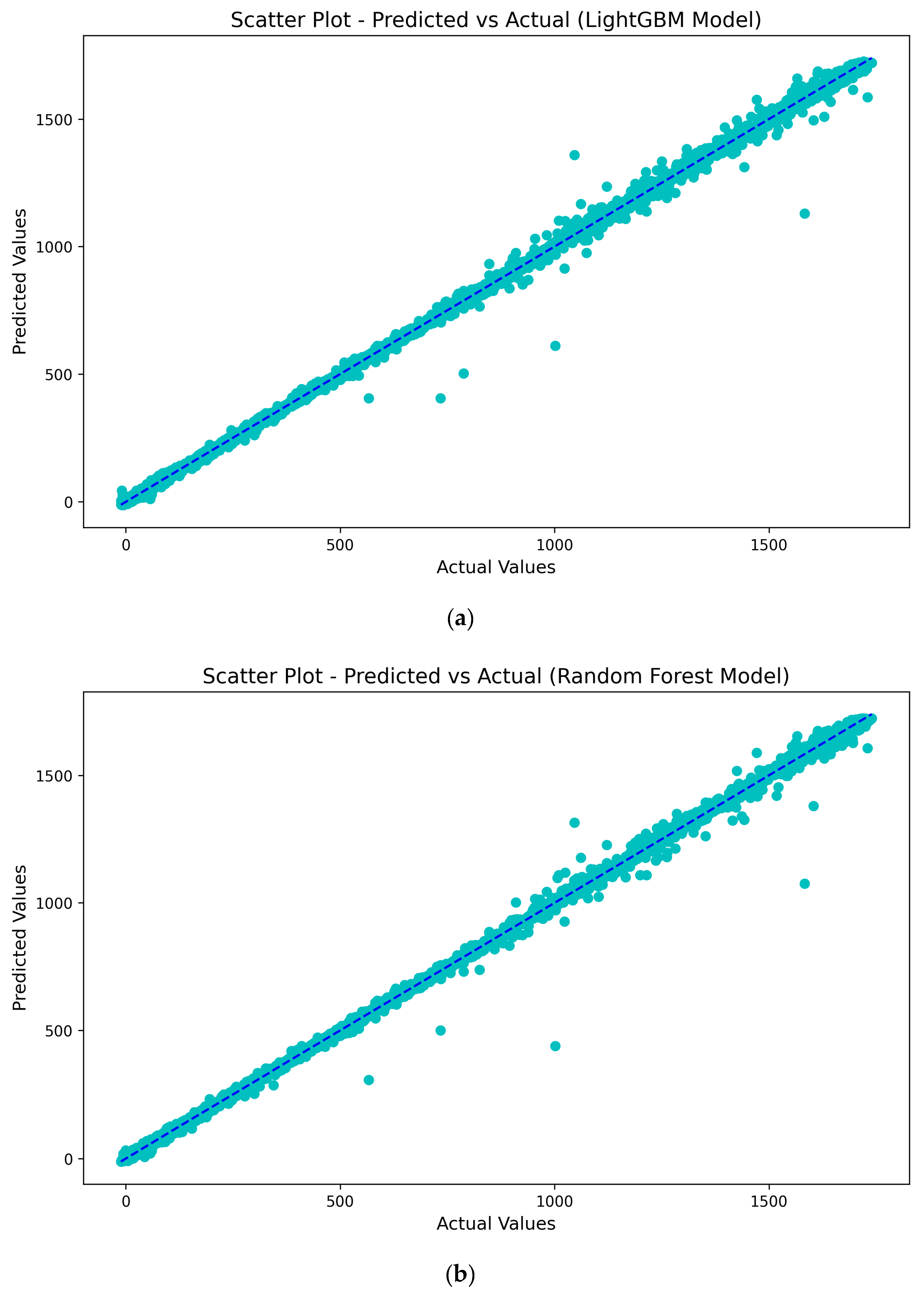
Figure 9 displays the residuals over time plots for each model, showcasing the difference between the predicted and actual values over time. These plots allow for the examination of patterns and trends in the residuals, providing insights into the models’ accuracy and potential areas of improvement. Figure 10 illustrates scatter plots comparing the predicted and actual values for each model. These plots visually depict the relationship between the predicted and actual values, demonstrating how well the models capture the true wind power values.
The accuracy and effectiveness of the proposed method heavily rely on the availability of high-quality and comprehensive data. Insufficient or incomplete data may limit the performance and generalizability of the model.

4. Conclusions

A prediction model was successfully developed, leveraging 16 different wind energy system parameters, to enable a more accurate and comprehensive prediction of short-term wind power. By utilizing state-of-the-art machine learning techniques, including LightGBM, random forest, CatBoost, and XGBoost, we achieved significant improvements in prediction performance. Through rigorous evaluation and comparison, we identified the CatBoost algorithm as the top-performing method for short-term wind power prediction. The 10-fold cross-validation results clearly demonstrate its superiority, with an impressive RMSE of 13.84 for the test set. This finding highlights the effectiveness and reliability of CatBoost for accurate wind power forecasting.
The developed short-term prediction model holds great potential for practical applications in grid control and turbine management. Accurate and timely wind power forecasts are crucial for optimizing grid stability, load balancing, and efficient turbine management, leading to improved overall performance and cost-effectiveness. Unlike many existing methods that rely on a limited number of features, our approach incorporates a wide range of characteristics by employing exploratory data analysis and heat map visualization. This allows us to identify and utilize relevant features while discarding irrelevant ones. Additionally, we implemented a procedure to remove outliers, ensuring data quality and enhancing the normal distribution of the dataset.
Looking ahead, we emphasize the need to explore deep learning techniques and expand the dataset to further enhance the model’s performance and applicability. These future directions will contribute to the ongoing development and advancement of wind power prediction methodologies.

Author Contributions

G.P. Conceptualization; Data curation; Roles/Writing—original draft; Investigation; Methodology, Formal analysis; Software; Visualization; S.J.: Supervision; Validation; K.K.: Writing—review & editing. All authors have read and agreed to the published version of the manuscript.

Funding

This research did not receive any specific grant from funding agencies in the public, commercial, or not-for-profit sectors.

Data Availability Statement

The dataset is available in publicly accessible database.

Conflicts of Interest

The authors declare no conflict of interest.

References

  1. Harindintwali, J.D.; Yuan, Z.; Wang, M.; Wang, F.; Li, S.; Yin, Z.; Huang, L.; Fu, Y.; Li, L.; Chang, S.X.; et al. Technologies and perspectives for achieving carbon neutrality. Innovation 2021, 2, 100180. [Google Scholar] [CrossRef]
  2. Ahmad, T.; Zhang, D. A critical review of comparative global historical energy consumption and future demand: The story told so far. Energy Rep. 2020, 6, 1973–1991. [Google Scholar] [CrossRef]
  3. Kulkarni, S.H.; Anil, T.R.; Gowdar, R.D. Wind Energy Development in India and a Methodology for Evaluating Performance of Wind Farm Clusters. J. Renew. Energy 2016, 2016, 6769405. [Google Scholar] [CrossRef] [Green Version]
  4. Dang, T. Introduction, history, and theory of wind power. In Proceedings of the 41st North American Power Symposium, Starkville, MS, USA, 4–6 October 2009; pp. 1–6. [Google Scholar] [CrossRef]
  5. Goudarzi, N.; Zhu, W.D. A review on the development of wind turbine generators across the world. Int. J. Dyn. Control 2013, 1, 192–202. [Google Scholar] [CrossRef] [Green Version]
  6. Xu, Y.; Li, Y.; Zheng, L.; Cui, L.; Li, S.; Li, W.; Cai, Y. Site selection of wind farms using GIS and multi-criteria decision making method in Wafangdian, China. Energy 2020, 207, 118222. [Google Scholar] [CrossRef]
  7. Gönül, Ö.; Duman, A.C.; Deveci, K.; Güler, Ö. An assessment of wind energy status, incentive mechanisms and market in Turkey. Eng. Sci. Technol. Int. J. 2021, 24, 1383–1395. [Google Scholar] [CrossRef]
  8. Wang, X.; Guo, P.; Huang, X. A Review of Wind Power Forecasting Models. Energy Procedia 2011, 12, 770–778. [Google Scholar] [CrossRef] [Green Version]
  9. Ramirez-Meyers, K.; Mann, W.N.; A Deetjen, T.; Johnson, S.C.; Rhodes, J.D.; Webber, M. How different power plant types contribute to electric grid reliability, resilience, and vulnerability: A comparative analytical framework. Prog. Energy 2021, 3, 033001. [Google Scholar] [CrossRef]
  10. Ragheb, M.; Ragheb, A.M. Wind Turbines Theory-The Betz Equation and Optimal Rotor Tip Speed Ratio. In Fundamental and Advanced Topics in Wind Power; IntechOpen: London, UK, 2011. [Google Scholar] [CrossRef] [Green Version]
  11. Barbosa de Alencar, D.; De Mattos Affonso, C.; Limão de Oliveira, R.C.; Moya Rodríguez, J.L.; Leite, J.C.; Reston Filho, J.C. Different Models for Forecasting Wind Power Generation: Case Study. Energies 2017, 10, 1976. [Google Scholar] [CrossRef] [Green Version]
  12. Ahmad, A.; Javaid, N.; Mateen, A.; Awais, M.; Khan, Z.A. Short-Term Load Forecasting in Smart Grids: An Intelligent Modular Approach. Energies 2019, 12, 164. [Google Scholar] [CrossRef] [Green Version]
  13. Baer, F. Numerical weather prediction. In Advances in Computers; Zelkowitz, M.V., Ed.; Elsevier: Amsterdam, The Netherlands, 2000; Volume 52, pp. 91–157. [Google Scholar] [CrossRef]
  14. Pearre, N.S.; Swan, L.G. Statistical approach for improved wind speed forecasting for wind power production. Sustain. Energy Technol. Assess. 2018, 27, 180–191. [Google Scholar] [CrossRef]
  15. Hong, Y.-Y.; Rioflorido, C.L.P.P. A hybrid deep learning-based neural network for 24-h ahead wind power forecasting. Appl. Energy 2019, 250, 530–539. [Google Scholar] [CrossRef]
  16. Gallego, C.; Pinson, P.; Madsen, H.; Costa, A.; Cuerva, A. Influence of local wind speed and direction on wind power dynamics–Application to offshore very short-term forecasting. Appl. Energy 2011, 88, 4087–4096. [Google Scholar] [CrossRef] [Green Version]
  17. Hodge, B.-M.; Zeiler, A.; Brooks, D.; Blau, G.; Pekny, J.; Reklatis, G. Improved Wind Power Forecasting with ARIMA Models. Comput. Aided Chem. Eng. 2011, 29, 1789–1793. [Google Scholar] [CrossRef]
  18. Peiris, A.T.; Jayasinghe, J.; Rathnayake, U. Forecasting Wind Power Generation Using Artificial Neural Network: “Pawan Danawi”—A Case Study from Sri Lanka. J. Electr. Comput. Eng. 2021, 2021, 5577547. [Google Scholar] [CrossRef]
  19. Singh, U.; Rizwan, M. Enhancing wind power forecasting from meteorological parameters using machine learning models. J. Renew. Sustain. Energy 2022, 14, 063302. [Google Scholar] [CrossRef]
  20. Zhang, Y.; Dong, Z.Y.; Kong, W.; Meng, K. A Composite Anomaly Detection System for Data-Driven Power Plant Condition Monitoring. IEEE Trans. Ind. Inform. 2019, 16, 4390–4402. [Google Scholar] [CrossRef]
  21. Kim, J.; Afzal, A.; Kim, H.-G.; Dinh, C.T.; Park, S.G. Wind power forecasting based on hourly wind speed data in South Korea using machine learning algorithms. J. Mech. Sci. Technol. 2022, 36, 6107–6113. [Google Scholar] [CrossRef]
  22. Tyass, I.; Khalili, T.; Rafik, M.; Abdelouahed, B.; Raihani, A.; Mansouri, K. Wind Speed Prediction Based on Statistical and Deep Learning Models. Int. J. Renew. Energy Dev. 2023, 12, 288–299. [Google Scholar] [CrossRef]
  23. Navas, R.K.B.; Prakash, S.; Sasipraba, T. Artificial Neural Network based computing model for wind speed prediction: A case study of Coimbatore, Tamil Nadu, India. Phys. A Stat. Mech. Appl. 2019, 542, 123383. [Google Scholar] [CrossRef]
  24. Amroune, M. Support vector regression-bald eagle search optimizer-based hybrid approach for short-term wind power forecasting. J. Eng. Appl. Sci. 2022, 69, 107. [Google Scholar] [CrossRef]
  25. Li, L.-L.; Cen, Z.-Y.; Tseng, M.-L.; Shen, Q.; Ali, M.H. Improving short-term wind power prediction using hybrid improved cuckoo search arithmetic-Support vector regression machine. J. Clean. Prod. 2020, 279, 123739. [Google Scholar] [CrossRef]
  26. Liu, Z.; Li, X.; Zhao, H. Short-Term Wind Power Forecasting Based on Feature Analysis and Error Correction. Energies 2023, 16, 4249. [Google Scholar] [CrossRef]
  27. Xu, P.; Zhang, M.; Chen, Z.; Wang, B.; Cheng, C.; Liu, R. A Deep Learning Framework for Day Ahead Wind Power Short-Term Prediction. Appl. Sci. 2023, 13, 4042. [Google Scholar] [CrossRef]
  28. Miele, E.S.; Ludwig, N.; Corsini, A. Multi-Horizon Wind Power Forecasting Using Multi-Modal Spatio-Temporal Neural Networks. Energies 2023, 16, 3522. [Google Scholar] [CrossRef]
  29. Zhu, A.; Zhao, Q.; Wang, X.; Zhou, L. Ultra-Short-Term Wind Power Combined Prediction Based on Complementary Ensemble Empirical Mode Decomposition, Whale Optimisation Algorithm, and Elman Network. Energies 2022, 15, 3055. [Google Scholar] [CrossRef]
  30. Lin, W.-H.; Wang, P.; Chao, K.-M.; Lin, H.-C.; Yang, Z.-Y.; Lai, Y.-H. Wind Power Forecasting with Deep Learning Networks: Time-Series Forecasting. Appl. Sci. 2021, 11, 10335. [Google Scholar] [CrossRef]
  31. Dataset Link. Available online: https://www.kaggle.com/datasets/theforcecoder/wind-power-forecasting (accessed on 11 February 2023).
  32. Ayilara, O.F.; Zhang, L.; Sajobi, T.T.; Sawatzky, R.; Bohm, E.; Lix, L.M. Impact of missing data on bias and precision when estimating change in patient-reported outcomes from a clinical registry. Health Qual. Life Outcomes 2019, 17, 106. [Google Scholar] [CrossRef] [Green Version]
  33. Qiu, P.; Niu, Z. TCIC_FS: Total correlation information coefficient-based feature selection method for high-dimensional data. Knowl.-Based Syst. 2021, 231, 107418. [Google Scholar] [CrossRef]
  34. Mukaka, M.M. Statistics corner: A guide to appropriate use of correlation coefficient in medical research. Malawi Med. J. 2012, 24, 69–71. [Google Scholar]
  35. Gress, T.W.; Denvir, J.; Shapiro, J.I. Effect of Removing Outliers on Statistical Inference: Implications to Interpretation of Experimental Data in Medical Research. Marshall J. Med. 2018, 4, 84. [Google Scholar] [CrossRef] [Green Version]
  36. Hair, J.; Black, W.C.; Babin, B.J.; Anderson, R.E. Multivariate Data Analysis, 7th ed.; Pearson Educational International: Upper Saddle River, NJ, USA, 2010. [Google Scholar]
  37. Byrne, B.M. Structural Equation Modeling with AMOS: Basic Concepts, Applications, and Programming; Routledge: New York, NY, USA, 2010. [Google Scholar]
  38. Irwanto, M.; Gomesh, N.; Mamat, M.; Yusoff, Y. Assessment of wind power generation potential in Perlis, Malaysia. Renew. Sustain. Energy Rev. 2014, 38, 296–308. [Google Scholar] [CrossRef]
  39. Liu, L.; Niu, M.; Zhang, C.; Shu, J. Light Gradient Boosting Machine-Based Link Quality Prediction for Wireless Sensor Networks. Wirel. Commun. Mob. Comput. 2022, 2022, 8278087. [Google Scholar] [CrossRef]
  40. Breiman, L. Random forests. Mach. Learn. 2001, 45, 5–32. [Google Scholar] [CrossRef] [Green Version]
  41. Kanagarathinam, K.; Sankaran, D.; Manikandan, R. Machine learning-based risk prediction model for cardiovascular disease using a hybrid dataset. Data Knowl. Eng. 2022, 140, 102042. [Google Scholar] [CrossRef]
  42. Mahesh, T.R.; Kumar, V.V.; Muthukumaran, V.; Shashikala, H.K.; Swapna, B.; Guluwadi, S. Performance Analysis of XGBoost Ensemble Methods for Survivability with the Classification of Breast Cancer. J. Sensors 2022, 2022, 4649510. [Google Scholar] [CrossRef]
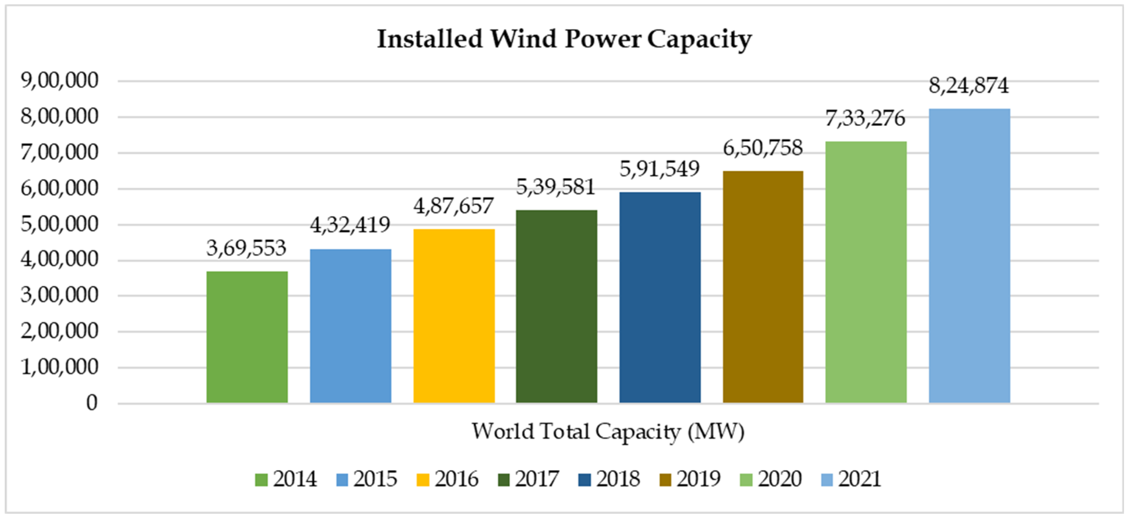
Figure 1. World total installed wind power capacity.
Energies 16 05459 g001
Figure 2. Block diagram of proposed approach.
Energies 16 05459 g002
Figure 3. Heat map illustrating the correlation between attributes in the wind power dataset.
Energies 16 05459 g003
Figure 4. Distribution of dataset features, skewness, and kurtosis values after outlier removal.
Energies 16 05459 g004aEnergies 16 05459 g004bEnergies 16 05459 g004c
Figure 5. Data distribution based on the wind power category.
Energies 16 05459 g005
Figure 6. Wind rose diagram.
Energies 16 05459 g006
Figure 7. Monthly mean values of (a) Gearbox Bearing Temperature; (b) Generator Winding1 Temperature; (c) Hub Temperature; (d) Nacelle Position; (e) Reactive Power; (f) Generator RPM; (g) Wind Speed; (h) Active Power.
Energies 16 05459 g007aEnergies 16 05459 g007bEnergies 16 05459 g007c
Figure 8. Daily mean value of wind speed.
Energies 16 05459 g008
Figure 9. Residuals over time plot of machine learning models for the prediction of Active Power: (a) LightGBM, (b) random forest, (c) CatBoost, and (d) XGBoost.
Energies 16 05459 g009aEnergies 16 05459 g009b
Figure 10. Scatter plot of the predicted and actual values of machine learning models for the prediction of Active Power: (a) LightGBM, (b) random forest, (c) CatBoost, and (d) XGBoost.
Energies 16 05459 g010aEnergies 16 05459 g010b
Table 1. Wind power prediction models.
Author(s)Type of ForecastingMethodEvaluation
Ying-Yi Hong et al. [15]24 h ahead wind power forecastingHybrid deep learning-based neural networkR2 = 0.8789 (summer),
0.8974 (fall), 0.9012 (spring) and 0.9125 (winter).
C. Gallego et al. [16]10 min forecastingAR model, CPARX and TARSO modelsCPARX (wind direction, wind speed) model—NRMSE ranged from 3.91 to 5.82.
AR Model—NRMSE ranged from 3.96 to 6.03.
TARSO (wind speed)—NRMSE ranged from 3.93 to 5.94.
Kim et al. [21]Daily wind power generation (hourly)ANN, kNN, RF, and SVRR2 varied from 0.97 to 0.98.
Tyass et al. [22]Medium-term forecastingForecasted the wind speed by combining the statistical SARIMA model with the deep neural network model.MAPE ranged from 10.50% to 15.94% for LSTM model and 10.67% to 16.10 for SARIMA model.
R Kaja Bantha Navas et al. [23]Medium-term forecastingDeveloped the categorical regression (CATREG) model, multilayer perception neural network (MLPNN) model, and RBFNN model for predicting wind speedMSE for MLPNN is 195.417, RBFNN is 3853.775, and for CATREG is 5598.937.
Amroune et al. [24]Short-term wind power forecastingEmployed hybrid strategy that is based on support vector regression and the bald eagle search optimizerR value 0.94574.
Ling-ling Li et al. [25]Short-term wind power predictionDeveloped the hybrid improved cuckoo search arithmetic—support vector regression machine (HICS-SVR)The regression fitting degree of the HICS-SVR is obtained under the condition of 100 iterations, with an average of 0.87 and an optimal value of 0.98.
Liu, et al. [26]Short-term wind power forecastingEmployed bidirectional long short-term memory network (BiLSTM)For wind farm A, RMSE as 0.9518 and MAPE as 2.3593.
For wind farm B, RMSE as 0.8537 and MAPE as 3.1740.
Xu, P et al. [27]A day-ahead wind power short-term prediction modelEmployed discrete wavelet transform—autoencoder—BiLSTMMAPE as 10.94 for wind farm #1, 13.30 for wind farm #2, 12.01 for wind farm #3.
Miele et al. [28]Multihorizon wind power forecasting modelA neural architecture based on stacked recurrent neural networks is proposedThe proposed model improved the XGBoost baseline with an average skill score of 25.1%.
Zhu et al. [29]Ultra-short-term wind power combined prediction modelComplementary ensemble empirical mode decomposition and the Elman neural network modelThe RMSE as 13.2642, MAE as 11.6409 and MAPE as 2.4158.
Lin et al. [30]Employed deep learning algorithm-based medium-term predictionTemporal convolutional networkMAPE as 5%.
Table 2. Descriptive statistics summary of the dataset.
IndexCountMeanStdMin25%50%75%Max
AmbientTemperatue93,81728.774.37025.6328.3431.6642.41
BearingShaftTemperature62,51843.015.55039.8442.9147.0155.09
Blade1PitchAngle41,9969.7520.64−43.16−0.940.398.1090.14
Blade2PitchAngle41,89110.0420.27−26.44−0.430.898.4890.02
Blade3PitchAngle41,89110.0420.27−26.44−0.430.898.4890.02
ControlBoxTemperature62,1600000000
GearboxBearingTemperature62,54064.2310.46057.8764.8371.0882.24
GearboxOilTemperature62,43857.566.32053.9457.2061.3170.76
GeneratorRPM62,2951102.03528.0601029.811124.861515.401809.94
GeneratorWinding1Temperature62,42772.4622.63055.4965.7985.87126.77
GeneratorWinding2Temperature62,44971.8322.65054.7665.0085.34126.04
HubTemperature62,40636.905.18033.9437.0040.0148.00
MainBoxTemperature62,50739.555.73035.8139.4943.3654.25
NacellePosition72,278196.2988.300145182271357
ReactivePower94,74888.13116.60−203.18−0.4335.88147.36403.71
RotorRPM62,1279.914.7209.2310.1013.6016.27
TurbineStatus62,9082280.43358,603.39022265,746,528
WindDirection72,278196.2988.300145182271357
WindSpeed94,5955.882.6203.825.567.5122.97
ActivePower94,750619.11611.28−38.5279.64402.651074.591779.03
Table 3. Wind power class classification based on wind speed.
Wind Power CategoryWind Speed (m/s)
Superb>8.8
Outstanding8 to 8.8
Excellent7.5 to 8
Good7 to 7.4
Fair6.4 to 7
Marginal5.6 to 6.3
Poor<5.6
Table 4. Wind power prediction models’ performance.
ML AlgorithmTraining Set (25,202, 16)Test Set (6301, 16)
MAEMSERMSER-Squared MAEMSERMSER-Squared
LightGBM6.034118.2110.870.9997.01248.4415.70.999
Random Forest2.3427.945.280.9996.462268.1316.370.999
CatBoost6.33988.449.4040.9997.781191.5713.840.999
XGBoost9.692307.6617.540.99910.431415.8520.390.998
Disclaimer/Publisher’s Note: The statements, opinions and data contained in all publications are solely those of the individual author(s) and contributor(s) and not of MDPI and/or the editor(s). MDPI and/or the editor(s) disclaim responsibility for any injury to people or property resulting from any ideas, methods, instructions or products referred to in the content.