Study of Combustor–Turbine Interactions by Performing Coupled and Decoupled Hybrid RANS-LES Simulations under Representative Engine-like Conditions

Abstract

Combustion–turbine interaction phenomena are attracting ever-growing interest in recent years. As a matter of fact, the strong unsteady and three-dimensional flow field that characterizes the combustor is usually conserved up to the first-stage nozzle, possibly affecting its design and performance in terms of aerodynamics and the effectiveness of the cooling system as well. Such conditions are also exacerbated by the employment of lean-burn combustors, where high turbulence levels are required for the flame stabilization, resulting in even greater temperature and velocity distortions at the inlet of the first-stage nozzle. Even if it has been proven by several past studies that the best way of studying the combustor–turbine interaction is simulating the two components together, performing coupled simulations is still challenging from a numerical point of view, especially in an industrial context. For this reason, the application and generation of the most representative and reliable boundary conditions possible at the inlet of the S1N have assumed an increased importance in order to study the two components separately by performing decoupled simulations. In this context, the purpose of the present work is to compare fully integrated combustor–stator SBES simulations to isolated stator ones. To perform the stator-only calculations, the fully unsteady inlet conditions of the stator have been recorded at the interface plane between the two components in the integrated SBES simulation and then they have been reconstructed by applying the proper orthogonal decomposition (POD) technique. The SBES simulations of the isolated stator have been so performed with the aim of determining whether the flow field obtained is comparable with the one of the integrated simulation, thus allowing more realistic results to be obtained rather than imposing time-averaged 2D maps, as per standard design practice.

1. Introduction

In recent years, numerous efforts have been made both through numerical and experimental studies in order to investigate the phenomena related to the interactions between combustors and turbines. As a matter of fact, several studies have shown that the vortical structures that characterize the combustor flow field are able to maintain a non-negligible part of its characteristics even at a relevant distance from the regions of the combustor where they are generated, in correspondence to the swirler. In particular, at the exit of the combustor, a highly non-uniform velocity distribution can be observed, characterized by high swirl and pitch components, along with temperature non-uniformities (“hot streaks”) [1] and high turbulence levels [2,3,4] that can be conserved up to the inlet of the following component, the first-stage nozzle of the high-pressure turbine (HPT), as proven both experimentally and numerically [5,6,7,8]. Such severe conditions are particularly exacerbated due to the employment of modern gas turbine (GT) combustors, such as lean-burning systems [9]. Such systems are indeed characterized by a very compact design, especially compared to the rich-quench-lean (RQL) ones, and by the potential reduction or absence of dilution holes due to a limited portion of air intended for the cooling of the liners. Moreover, high levels of turbulence are also necessary for flame stabilization to reach values up to 35% [5,6]. As a consequence, the interaction between the combustor and the turbine is governed by complex phenomena and the presence of such high swirled and turbulent hot impacting flow on the leading edge (LE) of the stator can potentially affect its aerodynamic and thermal behavior, which remains recognizable at the exit of the component, possibly impacting the rotor heat load and performance as well [10,11,12,13]. Moreover, the alteration of the behavior of the film cooling system causes a relevant increase in the metal temperature and thermal load of the first-stage nozzle (S1N), leading to a reduction in the component’s life. As a matter of fact, it has been proved by previous studies that the residual and high-swirl motion of the flow field outgoing from the combustor potentially provokes a variation in the local blowing ratio due to the resulting different distribution of the incidence and of the stagnation line on the LE [14,15,16,17,18,19,20].

For these reasons, an in-depth analysis of the phenomena related to combustor–turbine interactions is necessary for a robust and reliable aerothermal design of the first turbine stage. From a numerical point of view, the most reliable way to study such phenomena is performing unsteady fully coupled simulations [18,21], including both the combustor and the NGV in the computational domain. However, since the flow fields that characterize the two components are different, these simulations are quite challenging from a numerical point of view due to the different required spatial and temporal discretization. At the same time, studying the combustor and the NGV in a decoupled way can provoke significant inaccuracies, because the coupling effects are neglected in the prediction of the flow fields of both the components [22,23,24]. In the same way, the employment of a Reynolds-averaged Navier–Stokes (RANS) approach can introduce further approximations in the prediction of the thermal and flow fields due to the underprediction of the turbulent mixing that characterizes RANS simulations [25,26]. However, since RANS is able to limit the computational cost, it has historically played a central role in studying combustor–turbine interaction phenomena. For example, recently, to meet the goals of the STech (smart technologies) program, an annular sector rig, including a trisector non-reactive simulator and nozzle cascade, has been investigated by performing RANS simulations and then benchmarking the numerical findings to the available experimental results [4] in order to assess if traditional RANS modeling, usually employed for industrial best practice, is able to successfully predict the heat loads and the film cooling behavior on the S1N. It has been proven that instead more sophisticated CFD modeling should be considered.

In this context, a valid and more reliable alternative to RANS is represented by a large-eddy simulation (LES) [27,28,29], since it is able to resolve most of the turbulence scales and, thus, to provide high-fidelity solutions [30]. However, the employment of LES modeling results in a very high required computational cost due to the strict spatial and temporal discretization required. For this reason, its use is limited to simplified test cases, often suitable for laboratory applications, where realistic cooling systems are not equipped [31]. So, in light of this, hybrid RANS-LES turbulence models, such as scale-adaptive simulations (SASs) [32] and detached eddy simulations (DESs) [33,34], have started to play a relevant role in the most recent studies. For example, in the context of the project FACTOR (full aerothermal combustor–turbine interactions research), SAS simulations have been performed in order to study the aerothermal field on the vanes that were equipped on a non-reacting test rig of a lean-burn annular combustor. As a matter of fact, benchmarking the CFD predictions to the available experimental results obtained by Bacci et al. [20,35], Andreini et al. [2] demonstrated that SAS simulations describe the recirculating area inside the combustor better than RANS, thus improving the prediction of the turbulent mixing between the hot main flow coming from the combustor and the cooling flows [3]. An alternative to SAS and DES is represented by the stress-blended eddy simulation (SBES) model, that has become increasingly popular in recent years since it allows modeling of the boundary layers regions using RANS instead of using the more expensive LES, in terms of computational resources required [36]. For example, Verma et al. [37] simulated a coupled combustor–turbine configuration by using SBES. The results were then compared to those obtained by using RANS for only the NGV and SBES for only the combustor, noting that the decoupled approach is less efficient than the coupled one because an interactive procedure is necessary in order to converge the co-simulation model.

More recently, Tomasello et al. [38] used the SBES approach to simulate a fully integrated combustor–nozzle configuration under realistic operating conditions, equipped with a realistic turbine nozzle cooling system. The results were then compared to results obtained previously by performing an RANS, as per the standard design. In this case, as inlet boundary conditions for the NGV, time-averaged maps were prescribed by extracting them from a precursor SBES simulation of the stand-alone combustor, where a discharge convergent was placed to replace the NGV. The idea behind this operation was to preserve the throat area in order to obtain a realistic Mach number and back-pressure at the exit of the NGV. The main goal of the analysis was to fully study the behavior of the realistic film cooling system under representative and reactive operating conditions influenced by the interaction between the main hot flow coming from the combustor and the film cooling flow. The authors observed relevant differences in terms of film cooling adiabatic effectiveness on the NGV surface that could be associated with the strong underprediction of the turbulent mixing of the RANS modeling. As a matter of fact, even if the turbulent length scale values and distributions were comparable for the two simulations at the interface plane between the components, it was proven that the higher turbulent dissipation rate that characterized the RANS simulation ensured that the turbulent length scale decayed faster in the RANS case. Moreover, in order to fully study the impact of the presence of the combustor, a further numerical analysis was carried out by performing an SBES of the isolated NGV [39]. To achieve this, two-dimensional unsteady boundary conditions were prescribed at the inlet of the NGV, that were previously extracted from a high-fidelity available SBES simulation of the stand-alone combustor at runtime. By comparing the results to the fully integrated CC-S1N SBES simulation, it was noted that a non-negligible blockage effect of the NGV had a relevant impact on the velocity flow field inside the combustor, even sufficiently upstream from the interface plane that was chosen between the two components. Moreover, performing a high-fidelity CFD simulation of the NGV, taking into account also unsteady phenomena by imposing time-varying boundary conditions at the inlet of the NGV, seemed not to be sufficient to fully capture the behavior of the film cooling system. The main differences between the two simulations could be likely attributed to the fact that the two-dimensional unsteady boundary conditions were extracted from a decoupled simulation of the stand-alone combustor, hence, not taking into account the impact of the presence of the NGV on the flow field of the combustor.

The application and generation of the most representative and reliable boundary conditions at the inlet of the S1N have assumed an increased importance in studying combustor–turbine interaction phenomena in recent years. In particular, Duchaine et al. [40] performed an LES simulation of an integrated combustion chamber and the first turbine stage, then compared the results to LES simulations of the stand-alone turbine stage. As inlet boundary conditions for the turbine stage, two-dimensional mean maps extracted from the fully integrated case were imposed, without and with three different turbulence injections. The authors demonstrated that, even if the results seemed to be quite insensitive to the different turbulent injections, the CFD predictions obtained by simulating the stand-alone first stage were highly impacted by the imposed mean boundary conditions, confirming the importance of employing a coupled approach or imposing boundary conditions that are as realistic as possible. As a matter of fact, in the context of the project FACTOR, Martin et al. [41,42] generated a database of unsteady inlet boundary conditions under laboratory non-reactive conditions for the isolated NGV. To achieve this, the data were recorded at the interface plane between the combustor and nozzle from a fully coupled LES simulation including both components. The data were then post-processed and decomposed using advanced methods such as POD and SPOD in order to assess if such methods could be utilized to partially reconstruct the numerical database. Furthermore, recently Gründler et al. [43] presented a method to prescribe unsteady inlet boundary conditions by using proper orthogonal decomposition and Fourier series (PODFS) in order to preserve a realistic level of turbulence and unsteadiness at the stator inlet.

In this context, the purpose of the present work is to compare fully integrated combustor–stator and isolated stator SBES simulations. To do so, the fully unsteady inlet condition of the stator is recorded and reconstructed at the interface plane between the two components from the fully integrated SBES. Firstly, recorded snapshots are employed to recreate more realistic unsteady boundary conditions that are as representative as possible without any further post-processing operation. Then, the proper orthogonal decomposition (POD) technique is applied, taking into account three different numbers of POD modes (30, 10, 5) corresponding to a descending level of energy content (80%, 50%, 30%) with respect to the global turbulent kinetic energy. The results are then compared to an SBES of the stand-alone stator obtained by imposing time-averaged 2D maps from the fully integrated SBES simulation. In order to investigate the interaction between the combustor and the first-stage nozzle, numerical simulations are carried out under realistic operating conditions and geometry. As a matter of fact, the interaction between the main hot flow from the combustor and the cooling flows is studied by including a realistic turbine nozzle cooling system. Hence, all the SBES simulations of the isolated stator have been so performed with the aim of determining whether the flow field obtained is comparable with that of the integrated simulation, assumed as reference, allowing more realistic results to be obtained rather than imposing time-averaged 2D maps, as per standard design practice.

2. Proper Orthogonal Decomposition

Proper orthogonal decomposition (POD) is one of the data-driven modal analysis (DDMA) techniques, which aim to decompose an original dataset into a linear discrete combination of modes. For each mode, a defined temporal structure, depending on the values assumed by the mode in a specific point in different time instants, and a spatial one, depending on the values assumed by the mode in a specific time instant in different spatial locations, can be identified as well. This type of post-processing technique can be successfully used in order to identify the proper coherent structures of turbulent flows that are associated with the spatial distribution of each mode, and to reduce the complexity of the dynamics of a system, just taking into account the most important modes. In particular, POD is an energy-based decomposition which has as its main objective the approximation of the original dataset, expressed by the matrix $D(x,t)$, by using only the first $n_t$ modes, assuming the number of space points $n_s$ is significantly greater than the number of temporal instants $n_t$, as is common for most CFD applications. In this way, the energy content can be maximized, since these R modes are associated with the highest one. In particular, according to the so-called snapshot method, the matrix $D(x,t)$, as can be seen from Equation (1), is firstly obtained by recording the temporal and spatial evolution of selected quantities on a specified location, that can be a plane placed in a point of interest in the computational domain, as for this work. Each column of the matrix is, hence, made by a “snapshot” and looking at the columns corresponds to looking at the spatial distribution, while the temporal one can be read by looking at the rows of the matrix [44,45].

$$\begin{array}{c}\hfill D(x,t)=\left[\begin{array}{ccccc}{d}_{11}& \cdots & d_{1k}& \cdots & d_{1n_t}\\ ⋮& ⋮& ⋮& \ddots & ⋮\\ d_{n_{s}1}& \cdots & d_{n_{s}k}& \cdots & d_{n_s{n}_t}\end{array}\right]\end{array}$$

(1)

In particular, the POD technique allows the initial set of acquisitions $D(x,t)$ to be decomposed into a linear combination of orthogonal bases, the POD modes $\tilde{D}$, characterized by their own energy content ${\sigma }_k$, exclusively functions of time ${\psi }^T\left(t\right)$ and space ${\varphi }_k\left(x\right)$:

$$\begin{array}{c}\hfill D(x,t)=\sum _k{\varphi }_k\left(x\right)a_k\left(t\right)=\sum _k{\varphi }_k\left(x\right){\sigma }_k{\psi }^T\left(t\right)=\sum _k{\tilde{D}}_k\end{array}$$

(2)

In this way, it is possible to describe only the fluctuating part of the phenomenon under investigation. The quantities introduced by Equation (2) can be computed by reducing the initial problem to an eigenvalue problem of the matrix K, the so-called “temporal correlation matrix”, since it includes the correlations between the different snapshots, defined as follows:

$$\begin{array}{c}\hfill K=D^{T}D\end{array}$$

(3)

Still assuming $n_s>>n_t$, it is important to point out that it is possible to select a number of POD modes $\tilde{n}<n_t$ to correctly characterize the phenomenon, so introducing an approximation of the original matrix, characterized by a certain percentage of error.

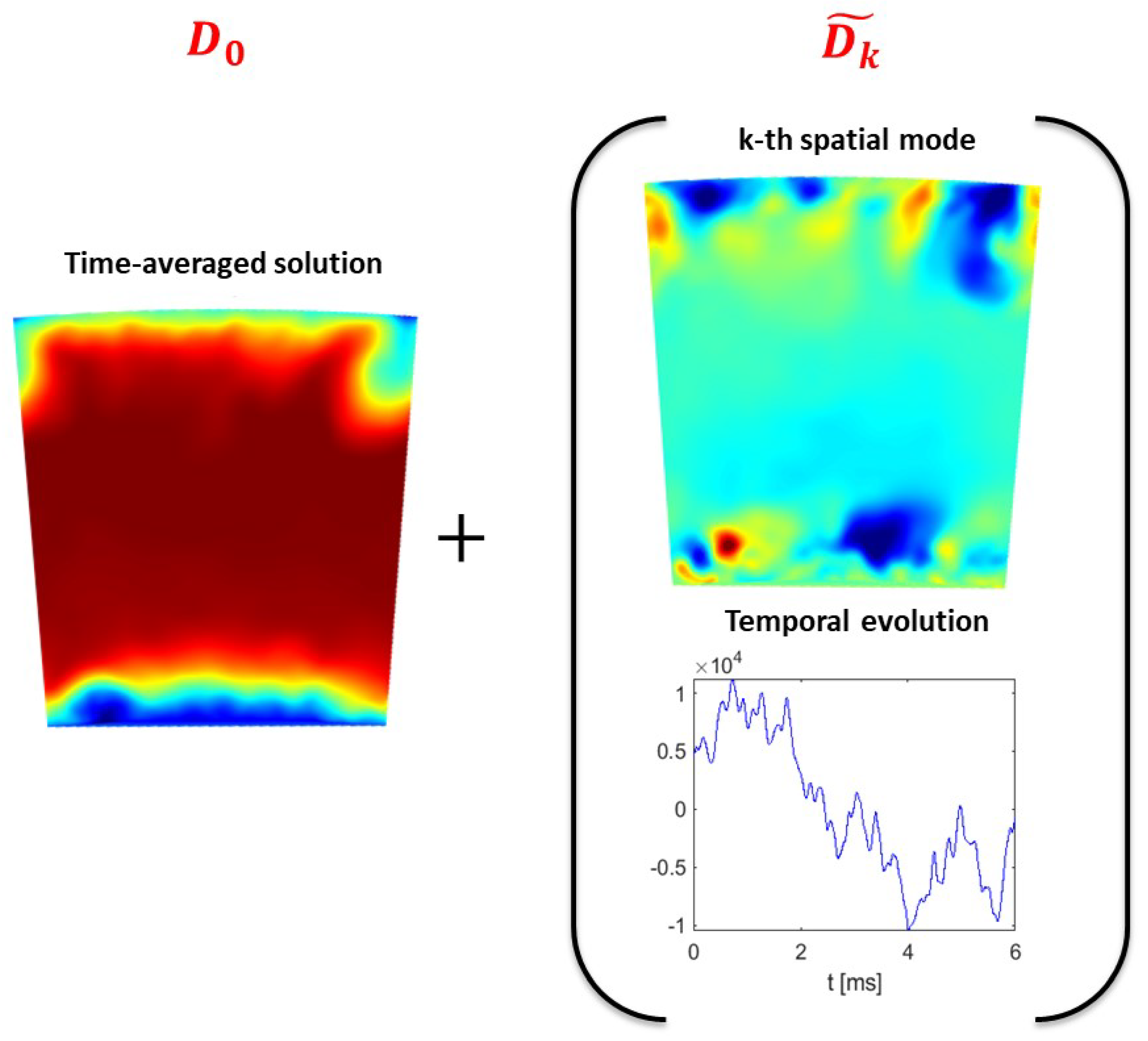
However, independently from the number of considered modes, the contribution of a k-th mode, defined as ${\tilde{D}}_k={\varphi }_k\left(x\right){\sigma }_k{\psi }_k^T\left(t\right)$, can be isolated starting from Equation (2). In order to assess the contribution of a generic mode $\widetilde{D_k}$, it is possible to algebraically combine it with the time-averaged field of the considered quantity, as can be seen from Figure 1. In this way, it is possible to assess how the specific mode under investigation alters the mean field, impacting the global behavior of the aerothermal field.

3. Combustion Model

The combustion model is based on the progress variable (c) transport equation, whose source term is calculated according to the turbulent flame speed ($S_t$) formulation [46]:

$$\begin{array}{c}\hfill {\overline{\dot{\omega }}}_c={\rho }_u{S}_t|\nabla \tilde{c}|\end{array}$$

(4)

with ${\rho }_y$ the density of the unburned mixture. The term $S_t$ can be determined according to Equation (5):

$$\begin{array}{c}\hfill S_t=u_{\Delta }^{{}^{\prime }3/4}{S}_c^{1/2}{\alpha }^{-1/4}{(C_S\Delta )}^{1/4}\end{array}$$

(5)

where $u_{\Delta }^{{}^{\prime }}$ and $(C_S\Delta )$ are, in the LES framework, the sub-grid-scale (SGS) fluctuation and the length scale, respectively, while $\alpha$ is the thermal diffusivity, and $S_c$ is the laminar flame speed in the original formulation of this combustion model. In the present study, the laminar flame speed is replaced by the consumption speed of the mixture [47,48]. The main advantage of adopting the consumption speed is the possibility to include the combined effect of the strain rate (a) and the heat loss ($\psi$) into the turbulent combustion model. Such a strategy allows the non-equilibrium effects to be accounted for, leading to an improvement in the prediction of the emissions, especially CO [49,50], and the flame extinction [51]. Leveraging the instantaneous solution, and not considering the curvature contribution that can be neglected at a high Karlovitz number, the strain rate can be calculated as:

$$\begin{array}{c}\hfill a=({\delta }_{i,j}-n_i{n}_j){\displaystyle \frac{\partial u_i}{\partial x_j}}\end{array}$$

(6)

with n being the flame front normal vector and $\left({\displaystyle \frac{\partial u_i}{\partial x_j}}\right)$ the velocity gradient. In the LES context, the grid-filtered contribution can be expressed according to Equation (7):

$$\begin{array}{c}\hfill {\tilde{a}}_{res}=({\delta }_{i,j}-\widetilde{n_i{n}_j}){\displaystyle \frac{\partial \widetilde{u_i}}{\partial x_j}}\end{array}$$

(7)

while the SGS-grid term, that quantifies the interaction between the flame front and the modeled vortexes, is calculated as follows:

$$\begin{array}{c}\hfill {\tilde{a}}_{sgs}={\Gamma }_k{\displaystyle \frac{\sqrt{k_{sgs}}}{\Delta }}\end{array}$$

(8)

where $k_{sgs}$ is the SGS-turbulent kinetic energy and $\Delta$ is the grid size. ${\Gamma }_k$ represents the efficiency function that models such an SGS interaction according to Meneveau et al. [52]. Equation (9) summarizes the mathematical formulation for the efficiency function, whose main terms are reported in Equations (10) and (11)

$$\begin{array}{c}\hfill {log}_{10}{\Gamma }_k=-{\displaystyle \frac{1}{s+0.4}}{e}^{-(s+0.4)}+(1-e^{-(s+0.4)})(s\sigma -0.11)\end{array}$$

(9)

$$\begin{array}{c}\hfill s={log}_{10}\left({\displaystyle \frac{\Delta }{{\delta }_l^0}}\right)\end{array}$$

(10)

$$\begin{array}{c}\hfill \sigma ={\displaystyle \frac{2}{3}}\left(1-{\displaystyle \frac{1}{2}}exp\left[-{\left({\displaystyle \frac{u_{\Delta }^{\prime }}{S_c}}\right)}^{1/3}\right]\right)\end{array}$$

(11)

with ${\delta }_l^0$ the laminar flame front thickness. From this formulation, it can be noticed that the flame front can be wrinkled only by vortexes whose characteristic size is at least 0.4 times the laminar flame thickness: smaller turbulent eddies are not able to penetrate or alter the flame front.

The enthalpy defect due to the heat loss effects is calculated considering the ratio between the actual cell-based value of the temperature with the adiabatic temperature that the cell would have at the same values of the mixture fraction Z, the progress variable, and their corresponding variances:

$$\begin{array}{c}\hfill Z={\displaystyle \frac{\tilde{T}(Z,Z^{{}^{″}2},c,c^{{}^{″}2},h)}{{\tilde{T}}_{ad}(Z,Z^{{}^{″}2},c,c^{{}^{″}2},h_{ad})}}\end{array}$$

(12)

During the time step of the LES, the consumption speed value to be associated with the cell can be read from a pre-computed table accessed through the local value of the mixture fraction, strain rate, and heat loss according to the above reported equations. The table is built by running several one-dimensional premixed flames in Cantera [53] where each parameter $(Z,a,\psi )$ is varied independently. In Cantera, the strain rate is progressively increased, raising the velocity of the two opposite jets (fresh mixture on one side and its products on the opposite side), while the enthalpy defect is simulated by decreasing the temperature of the combustion products. In total, three “for” cycles are used to independently vary these quantities and obtain the 4-dimensional table $S_c$$(Z,a,\psi )$. Both Cantera and the CFD simulations employ the GRI-3.0 [54] as the chemistry set and, obviously, the same operating conditions in terms of operating pressure, temperature of the oxidizer, and using pure methane as the fuel.

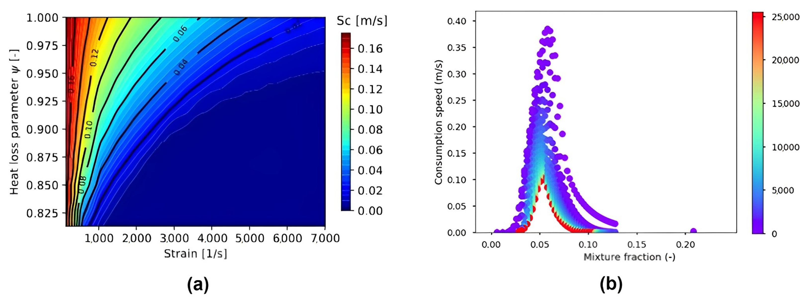
Figure 2 shows an example of the consumption speed map as a function of $a-\psi$$\left(a\right)$ and $Z-a$ in adiabatic conditions $\left(b\right)$. Figure 2a is particularly useful to capture the impact of the strain in the presence of heat loss. In fact, even when the heat loss is weak, the rising of the strain rate leads rapidly to the flame extinction $S_c\approx 0$; on the contrary, moving close to adiabatic conditions, the flame-out of the 1D flame is reached for $a>>$ 7.000 1/s.

4. Turbulence Model

For all the performed runs, the turbulent model used is the stress-blended eddy simulation (SBES), allowing the RANS approach to be applied only close to the boundary layer and the LES in the core of the flow with the dynamic-Smagorinsky algorithm for the turbulent SGS modeling.

All the computational analyses have been carried out by using the commercial code 3D Navier–Stokes solver Ansys Fluent v21.1. Referring to the numerical schemes, all the equations, including the time step advancements, are treated at the second order, while a coupled scheme is adopted for the pressure–velocity coupling. The choice of the time step size is driven by the velocity of the flow at the S1N throat (where the Mach number reaches a value well above 0.8) and by the constraint not to exceed a value of 3 for the Courant number in this section.

5. Computational Model

5.1. Combustor-S1N Case

The numerical analysis is performed considering a single sector of the NOVA LT16 ®annular combustor (Figure 3). Unfortunately, the number of swirlers and the number of first-stage nozzles (S1N) are prime each other; since the simulation of the full annular ring is too expensive from a computational standpoint, the geometry of the S1N is slightly modified to be included in a single sector of the combustion arrangement. The geometry is stretched but the pitch–chord ratio as well as the throat area are kept at the same values of the original design to preserve the fidelity of the numerical model with the real stator.

As represented by Figure 3, the geometry employed for the analysis includes all the main features, not only of the S1N but also of the interfaces between the combustor and the stator. Such interfaces are modeled through the cavities where the seals are installed: the leakages between two pairs of seals are considered as well in the model, imposing the corresponding mass flow rate in a dedicated inlet. Such a mass flow rate, as well as all the other mass flow rates at the different sections of the combustor and the S1N, come from a flow network model. Looking at the S1N more closely, the model includes all the cooling flows not only of the blade but also of the outer and inner platforms. Such flows have to be included not just to investigate the solution related to the platforms but also to understand their interaction with the cooling flows of the airfoil and with the flow coming out from the cavities. Regarding the cooling of the stator, the number of holes on both sides of the airfoil is preserved if compared to the real design, while the position is slightly different as a consequence of the above mentioned scaling of the geometry.

The model of the combustor starts from the compressor discharge chamber placed upstream of the premixer (not visible in Figure 3): the inclusion of this component allows the flow fluctuations at the burner entrance to be properly modeled. The burner is simulated considering all the details of the counter-rotating swirler [55], inside which the main fuel is injected to create the premixed mixture. The burner is equipped also with a pilot fuel line responsible for the flame stabilization in the primary zone of the dome. In the present study, the fuel composition is assumed to be pure methane. Despite this being a simplified assumption, pure methane can represent a good candidate for the mean natural gas composition that can include high C2+ elements but also inert elements. The liners include the cooling holes at all the sections of the combustor. For example, in Figure 3, the film cooling associated with the final part of the liners close to the cavities can be observed.

As previously mentioned, a mass flow inlet-type boundary condition is employed for each inlet along the domain while the outlet is a standard pressure outlet with the expected pressure drop associated with the flow expansion in the stator imposed. The latter information is known since the conditions corresponding to the ISO base load of the engine are considered for the investigation.

The final mesh count is equal to 81 million polyhedral elements. Such a high number is due to an extremely fine resolution in the combustor (especially in the primary zone, the burner, and at the fuel inlets [56]) and inside the S1N. Moreover, 14 prism layers are created at the walls with the goal of limiting the $y^{+}$ to 1 in the boundary layer. Figure 4 shows the mesh in the primary zone and inside the first-stage nozzle through a longitudinal view of the middle plane of the combustor; furthermore, a blade-to-blade section is reported to better highlight the mesh resolution in the stator.

The verification of the goodness of this mesh resolution is made through the calculation of Pope’s criterion [57]. Adopting a rigorous approach, such a parameter has to be looked at only in the core of the flow, far from the walls where the large-eddy simulation (LES) is resolved, and it can be calculated as follows:

$$\begin{array}{c}\hfill {\displaystyle \frac{k_{res}}{k_{res}+k_{sgs}}}\end{array}$$

(13)

with $k_{res}$ the resolved part of the turbulent kinetic energy spectrum and $k_{sgs}$ the modeled one evaluated through the SGS viscosity:

$$\begin{array}{c}\hfill k_{sgs}={\left({\displaystyle \frac{{\mu }_{sgs}}{{\rho }_{l_{sgs}}}}\right)}^2={\left({\displaystyle \frac{{\mu }_{sgs}}{\rho C_s\Delta }}\right)}^2\end{array}$$

(14)

More information regarding the conservation and turbulence equations peculiar to the numerical model used can be found in [36,58]. The contour plot of Figure 5 reports the calculated Pope’s criterion on the stator. Moving in the flow direction, the index is well above 0.9 inside the combustor and remains higher than 0.8 inside the nozzle; so, the prescription to resolve at least 80% of the turbulent kinetic energy is fully accomplished. Only the regions close to the wall, where the RANS is solved, remain below such a threshold. With regard to this, a thickening of the boundary layer can be observed in the suction side of the airfoil where the solution is solved as RANS.

5.2. S1N Case

The numerical grid of the S1N stand-alone is exactly the same as the mesh of this component in the integrated configuration, since a cutting plane at the p395 was placed to isolate the stator, corresponding to the inlet of the component. The final mesh count of the isolated S1N is equal to approximately 20 million polyhedral elements, including 14 prismatic layers. In addition, the SBES numerical calculations of the S1N stand-alone case share the same features in terms of general setup. In order to represent the high levels of turbulence and temperature distortions that characterize the combustor’s outlet, a set of two-dimensional time-varying boundary conditions have been imposed. To achieve this, at the interface plane p395 between the combustor and the turbine, a set of instantaneous quantities have been extracted from the integrated SBES simulation. In particular, the data have been stored every 0.015 ms over a period of time of 25 ms, that covers approximately almost two FTT of the isolated combustor and 25 FTT of the isolated NGV domains. In this way, it has been possible to maintain a satisfactory temporal discretization and at the same time limit the data size. However, just a portion of the recorded data has been used for the generation of the unsteady boundary conditions for the stator-only model. In particular, a portion corresponding to about 6 ms has been selected (6 FTT of the isolated S1N) due to the reduced FTT that characterizes the stand-alone stator, so keeping the computational effort contained. The plane selected as the interface is made of 22,172 nodes. As an example, Figure 6 represents the instantaneous total temperature at the S1N inlet at the instant $t_1$ and the instant $t_2=t_1+100t_s$, where $t_s$ is the adopted time step.

Each snapshot records information about the mass flow ($\rho u_x$, $\rho u_y$, $\rho u_z$), velocity ($u_x$, $u_y$, $u_z$), total temperature, and turbulence quantities, the mixture fraction and the progress variable. Moreover, also a passive scalar has been included in order to track the film cooling concentration coming from the nuggets. Regarding the inlet boundary conditions, for all the S1N stand-alone simulations, the mass flow, in terms of mass flux, the flow directions, and the total temperature have been imposed at the S1N inlet, along with the turbulent quantities previously extracted. Regarding the outlet, the same static pressure profile of the integrated SBES calculation has been imposed at the domain’s outlet. Since one of the main goals of this analysis is to assess the capability of the stand-alone S1N SBES simulation to capture the flow field characteristics of the fully integrated SBES simulation, different boundary conditions have been imposed at the stator inlet:

• Firstly, the recorded snapshots are employed to recreate realistic and as representative as possible unsteady boundary conditions without any further post-processing operation.
• Then, the POD technique is applied, taking into account three different POD modes:

  −

  The first thirty POD modes are identified and imposed at the S1N inlet. They represent approximately 80% of the energy with respect to the fully integrated SBES simulation, assumed as reference. It is important to point out that POD is applied individually on all the quantities prescribed at the S1N inlet as mentioned above.

  −

  The first ten POD modes are identified and imposed at the S1N inlet. They represent approximately 50% of the energy.

  −

  The first five POD modes are identified and imposed at the S1N inlet. They represent approximately 30% of the energy.

• Finally, a further SBES analysis has been included in this work, imposing as inlet boundary conditions two-dimensional maps by time-averaging the unsteady boundary conditions prescribed at the previously described S1N SBES calculations. This simulation can be considered as the application of the standard industrial practice in the case of an unsteady SBES calculation.

To recap, the main parameters regarding the setup of all the CFD simulations are summarized in

Table 1. Summary of the main parameters of the setup of the CFD simulations. (©2023 Baker Hughes Company—All rights reserved).

CFD Simulation	CFD Domain	Inlet BCs
SBES CC+S1N	CC+S1N	Mass flow inlets
SBES S1N	S1N	Set of instantaneous 2D maps from SBES CC+S1N
SBES S1N 30POD	S1N	Set of instantaneous 2D maps from SBES CC+S1N (first 30 POD modes)
SBES S1N 10POD	S1N	Set of instantaneous 2D maps from SBES CC+S1N (first 10 POD modes)
SBES S1N 5POD	S1N	Set of instantaneous 2D maps from SBES CC+S1N (first 5 POD modes)
SBES S1N timeavg	S1N	Time-averaged 2D maps from SBES CC+S1N

:

6. Operating Conditions

All the simulations are performed according to realistic engine-like operating conditions, corresponding to a condition of full speed and load for the engine during the FEET campaign. The most interesting information regarding the operating conditions is summarized in

Table 2. Summary of the main parameters of the operating conditions taken as reference for all the SBES calculations presented here. (©2023 Baker Hughes Company—All rights reserved).

Test Point Conditions
Fuel Composition (% vol.)	CH4	87
	C2+	7.5
	Inert	5.5
Pilot/Premix fuel ratio (-)	0.36
Ambient Temperature (°C)	6
Firing Temperature	Design Value
TNH, TNL (%)	100

. While keeping the fire temperature at the design value, the pilot/premix fuel ratio has been chosen in order to limit the NO15 emission to below 15 ppmv. Moreover, as can be observed, the C2+ and the inert content are kept limited for the fuel composition.

7. Results

7.1. Analysis of the Application of Time-Varying Boundary Conditions at S1N Inlet

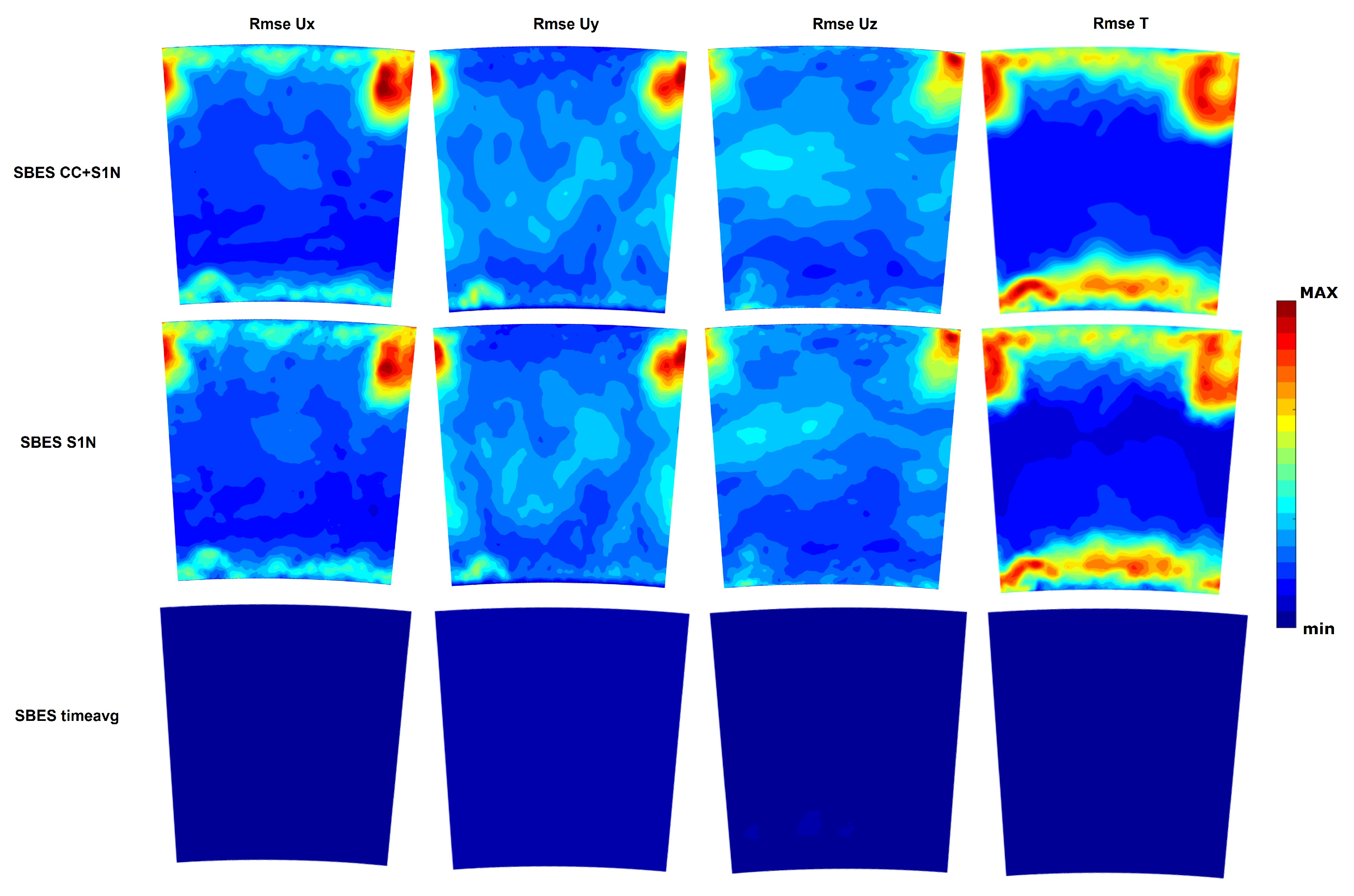
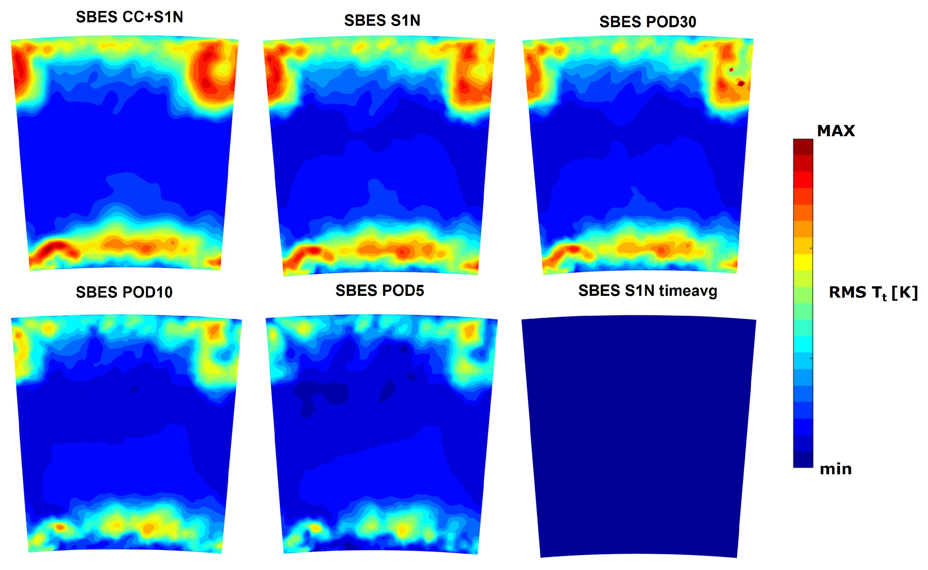
Firstly, before applying the POD technique, the focus lies on the ability of time-varying boundary conditions to reconstruct the flow field at the interface plane between the combustor and the turbine simulated by the integrated simulation. To achieve this, the RMS U_x, RMS U_y, RMS U_z, and RMS T_t are presented in Figure 7 for S1N SBES and S1N timeavg calculations, then compared with SBES CC+S1N, selected as a reference.

Looking at the RMS U_x, RMS U_y, and RMS U_z, it is clear that the SBES S1N results fall very close to those from SBES CC+S1N. This confirms that the applied time-varying boundary conditions are able to successfully replicate the turbulence kinetic energy at the inlet of the stator, contrary to what happens with constant boundary conditions (SBES timeavg). Similar considerations can also be made by looking at the RMS T_t results. It is, therefore, possible to conclude that the time-varying boundary conditions, applied in the manner described above, are able to satisfactorily reproduce the fluctuations of the velocity and temperature fields typical of the integrated simulation. In order to quantify the similarities between SBES CC+S1N and SBES S1N, the velocity components and their respective RMS values, the normalized total temperature, and the total temperature RMS values are reported in

Table 3. Averaged values obtained at plane 39.5 for the three velocity components and the respective RMS, normalized total temperature, and the total temperature RMS are reported for SBES CC+S1N and SBES S1N. The relative differences between the two cases are also included. (©2023 Baker Hughes Company—All rights reserved).

	SBES CC+S1N	SBES S1N	Relative Difference
U (m/s)	59.848	60.466	1.032%
RMS U (m/s)	12.596	12.226	−2.941%
$U_x$ (m/s)	56.186	56.788	1.072%
	6.176	6.081	−1.527%
$U_y$ (m/s)	−17.417	−17.673	1.471%
RMS $U_y$ (m/s)	6.614	6.518	−1.447%
$U_z$ (m/s)	−3.543	−3.246	−8.390%
RMS $U_z$ (m/s)	8.430	8.027	−4.774%
$T_{t,nd}$ (-)	0.852	0.849	−0.397%
RMS $T_t$ (K)	0.861	0.849	−1.489%

by performing a spatial averaging at plane 39.5. The total temperature was normalized as follows:

$$\begin{array}{c}\hfill T_{t,nd}={\displaystyle \frac{T-T_{min}}{T_{max}-T_{min}}}\end{array}$$

(15)

As can be seen, the relative differences between SBES S1N and SBES CC+S1N, selected as reference, are lower than 5% for all the quantities, with the exception of U_z. Since the obtained quantities are strictly related to the imposed inlet boundary conditions for the SBES S1N case, this confirms once again that this set of boundary conditions is able to reproduce the flow field characteristics of SBES CC+S1N in a realistic and representative way.

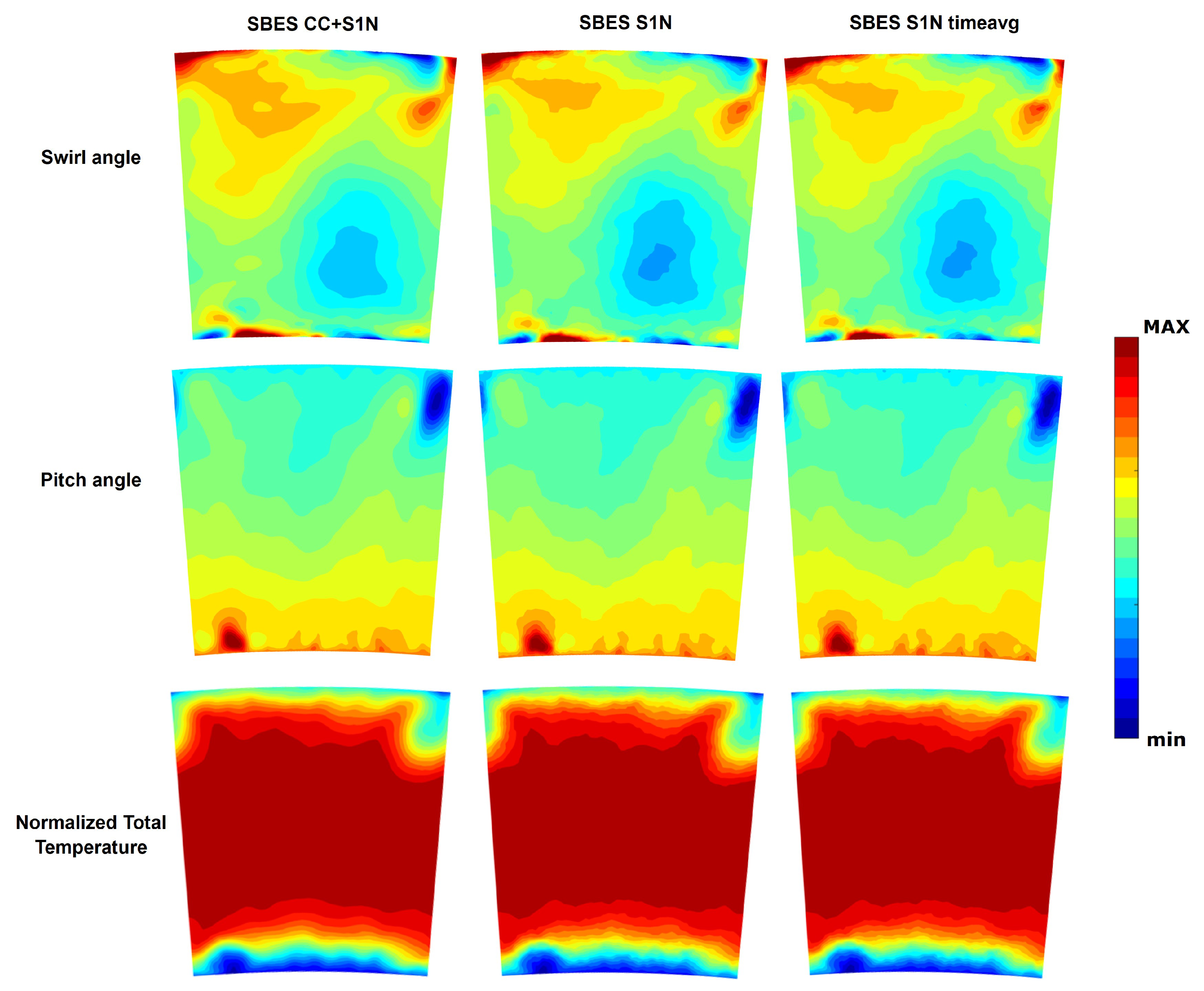
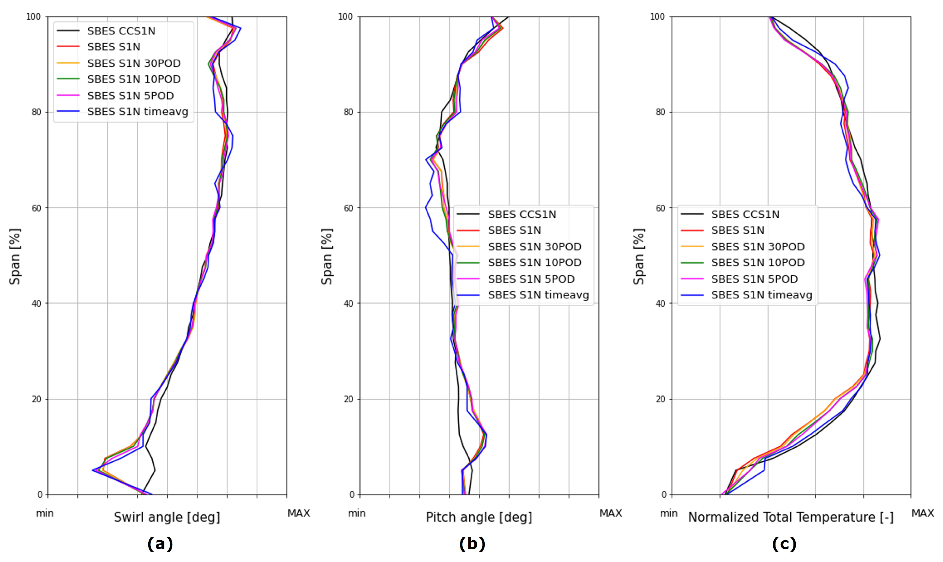
Moreover, it is also important to point out that the inlet boundary conditions for the selected simulations are equal in terms of averaged values, since, as anticipated, the inlet boundary conditions for SBES timeavg are obtained by time-averaging the unsteady boundary conditions prescribed for the S1N SBES calculation. So, in order to visualize it better, the three simulations have been further compared by looking at the normalized total temperature, swirl, and pitch angle distributions at the S1N inlet. In particular, the quantities are defined as follows:

$$\begin{array}{c}\hfill swirl=arctan\left({\displaystyle \frac{V_{tan}}{V_{ax}}}\right)\end{array}$$

(16)

$$\begin{array}{c}\hfill pitch=arctan\left({\displaystyle \frac{V_{rad}}{V_{ax}}}\right)\end{array}$$

(17)

As can be noted from Figure 8, as expected, the contours present very similar behavior.

7.2. Pod Sensitivity Analysis

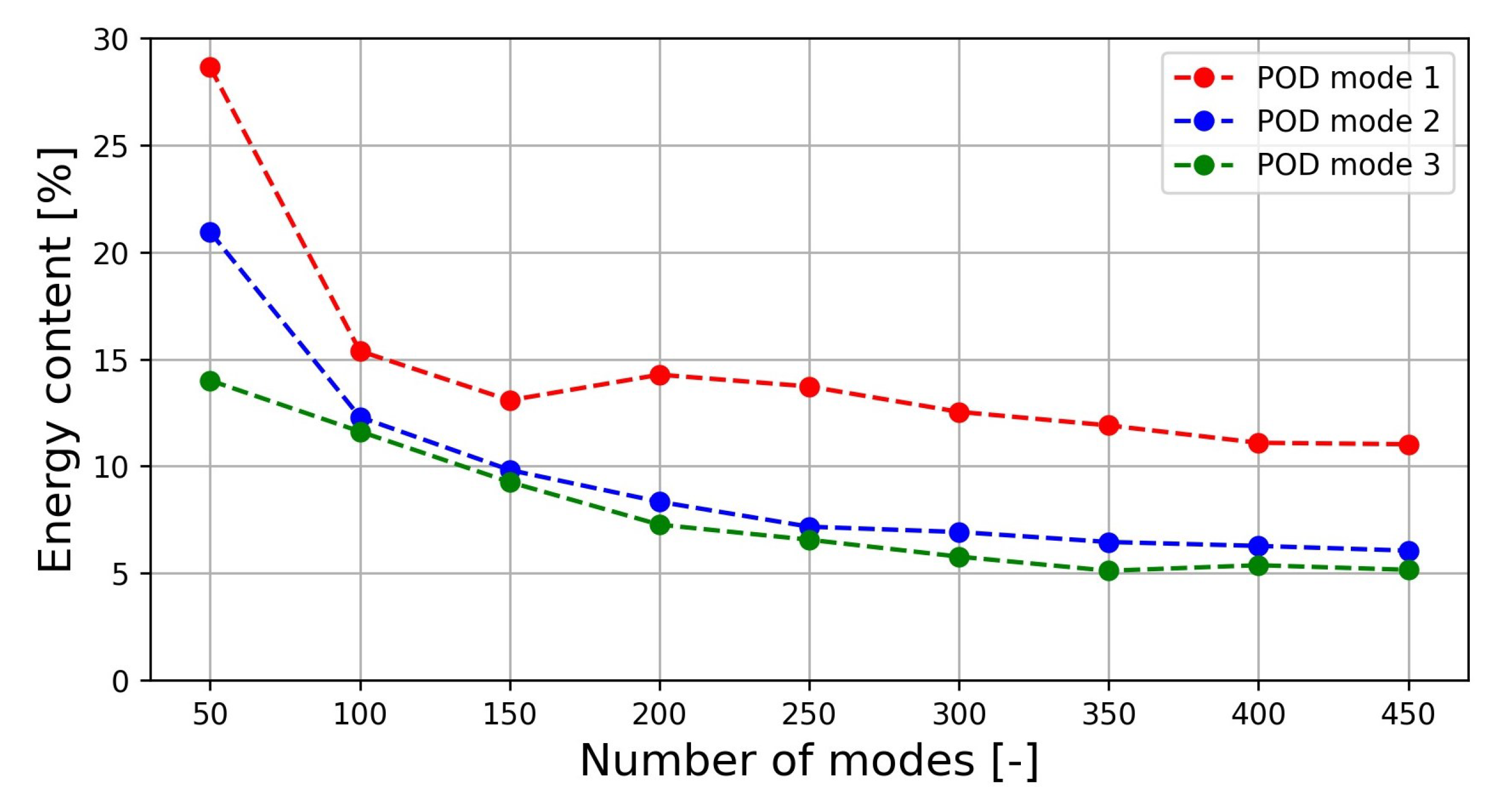
As anticipated, the data have been recorded every 0.015 ms over a period of 25 ms, corresponding to snapshots. However, a reduced number of modes have been considered for the calculation of the truncated correlation matrix in order to keep the computational effort contained. Hence, firstly, an analysis of sensitivity for the definition of the number of snapshots is presented here, as was performed in a previous study [59]. To achieve this, the POD technique is applied to the mass flux $\rho u_x$ on the plane 39.5, since it has been prescribed as the inlet boundary condition for the S1N simulations, assessing the energy content and dominant frequency of the first tree modes. The results are presented in Figure 9. As can be seen, the turbulent kinetic energy of the first three modes does not vary significantly from 400 to 450 modes, with an energy content of approximately 11%, 6%, and 5% of the total for the first, second, and third modes, respectively.

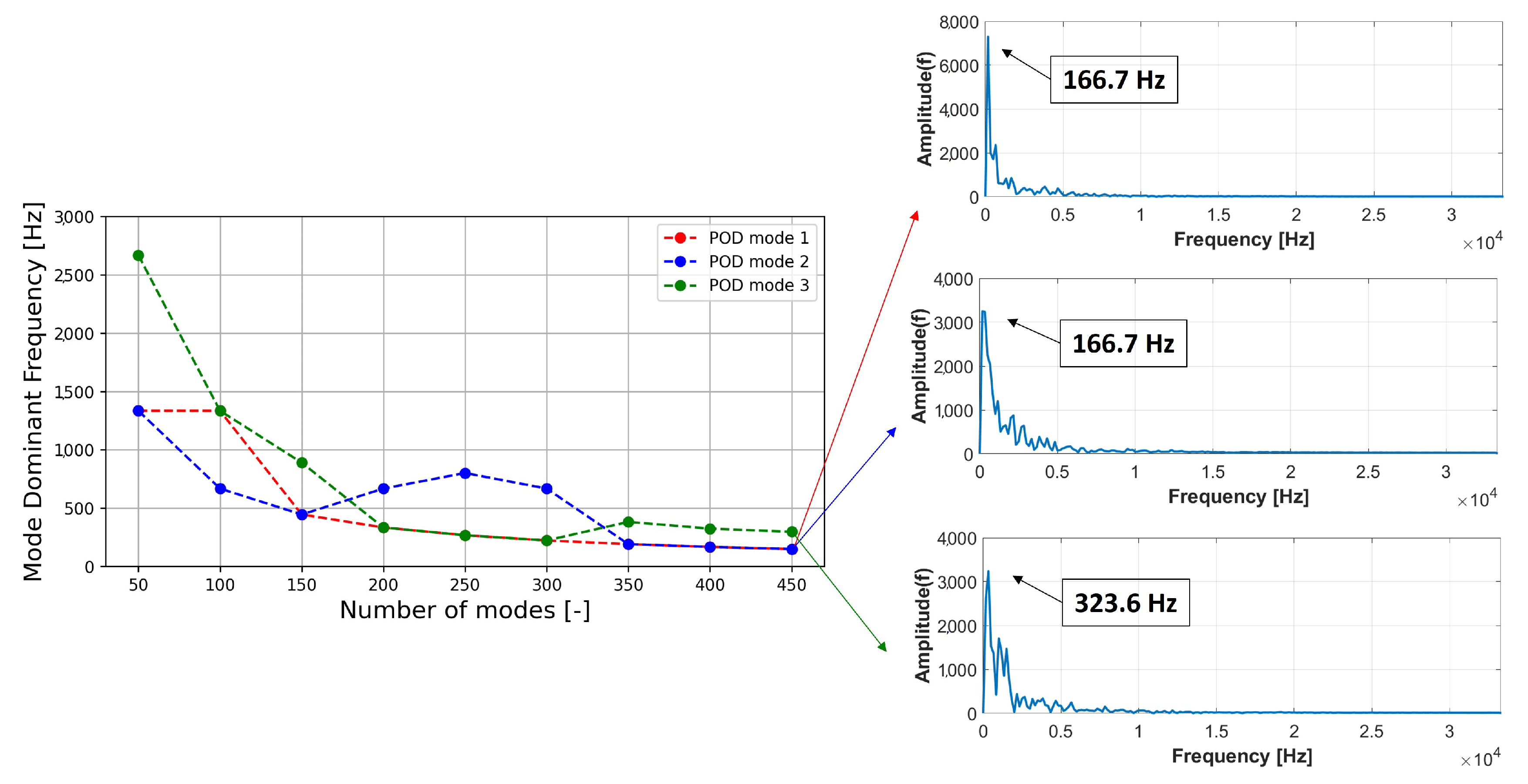
Regarding the dominant frequency, the results are summarized in Figure 10. Taking into account more than 350 modes, the first two modes are associated with the same constant dominant frequencies of about 166.7 Hz. Looking at the third one, similar conclusions can be drawn, even if it is characterized by a slightly more evident variation in terms of the dominant frequency between 350 and 400 modes. Thus, in conclusion, 400 modes have been selected for the following calculations.

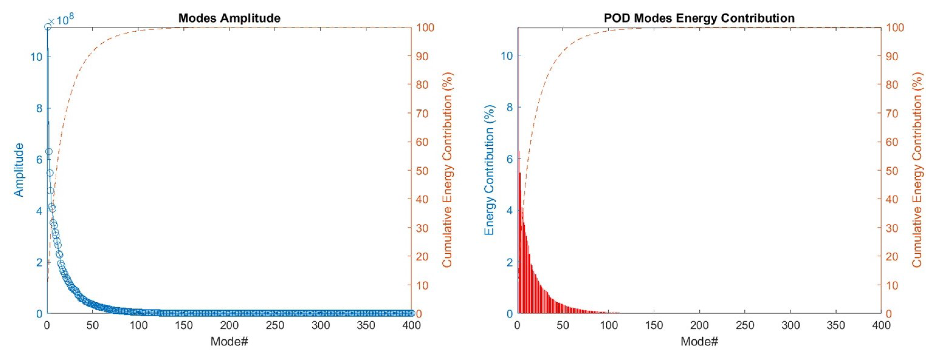
As anticipated, since POD analysis allows the extraction of the energy content of each mode, it can be used to indicate the most important ones to reproduce the overall dynamics of the flow. In this context, Figure 11 represents the characteristics of each mode, in terms of amplitude and energy contribution. As can be seen, the first five modes contribute largely to the dynamics of the flow; after these, the energy content associated with the following modes starts to decay very slowly, indicating that the first five modes could be enough to capture the most important coherent structures of the aerothermal field. In particular, the first mode is the principal mode, and it is responsible for 11% of the energy content, and globally the first five modes correspond to 30% of the total turbulent kinetic energy.

7.3. Interpretation of the POD Modes

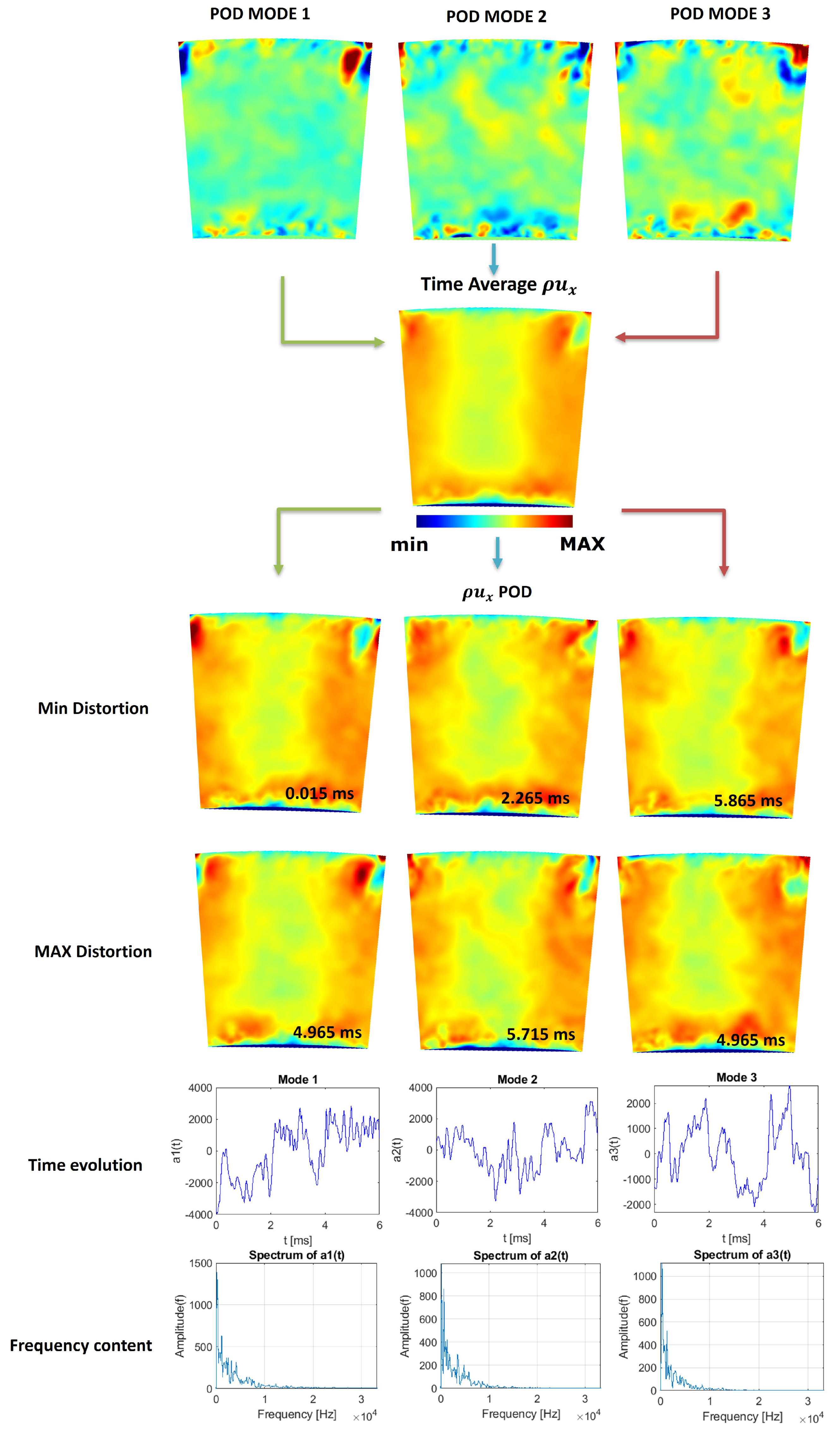
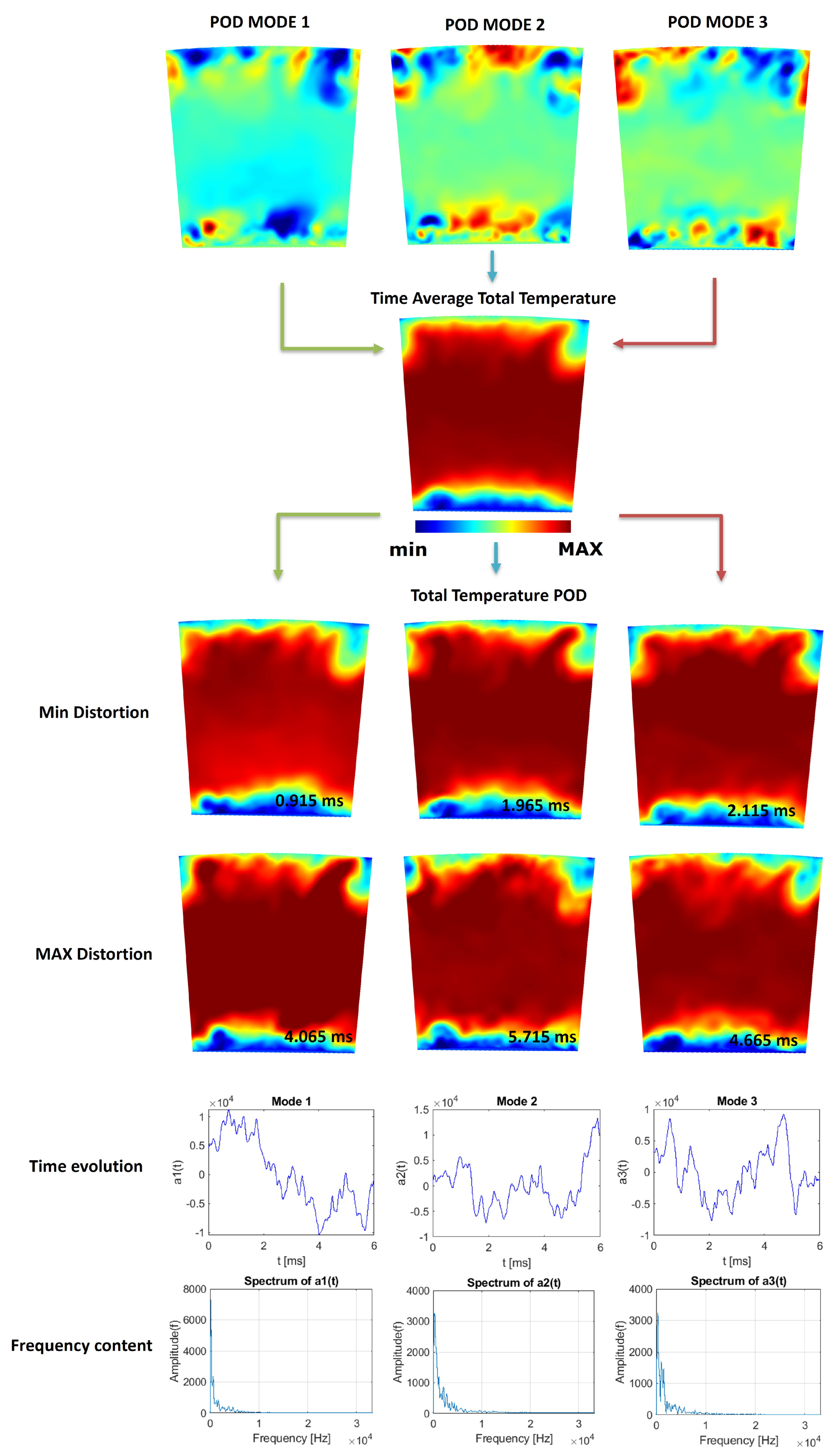
To better understand the coherent structures that can be identified by the POD modes, Figure 12 reports the most relevant information for $\rho u_x$ in terms of both the spatial and temporal modes for the first three coherent structures. The analysis has been limited to the first three POD modes for the sake of brevity. To better quantify the results, the minimum and maximum distortions of the $\rho u_x$ field is reported with respect to the time-averaged field. To achieve this, each POD mode is algebraically summed to the time-averaged solution obtained for all the collected time history. Looking at the time-averaged field, an evident blockage effect can be noted due to the presence of the leading edge (LE) of the following first-stage stator. As a matter of fact, according to [38,39], the presence of the LE results in a strong deceleration in this region, that can be clearly observed in the central portion of the plane 39.5. This is clearly compensated for by a non-negligible acceleration around the LE. In this context, the POD modes show fluctuations in the flow field mainly limited to the endwalls, above all where there is the cooling flow coming out from the nuggets, preserving thus, as expected, the central area of plane 39.5 where the blocking phenomenon is highlighted. As a matter of fact, the minimum and maximum distortions of the flow show at most some expansions and contractions of the flow field in correspondence to this zone, always compensated for by local accelerations and decelerations around the LE to guarantee the average conservation of the total mass flow. As far as the endwalls are concerned, greater fluctuations are instead evident for all POD modes considered, thus underlining how the greater levels of turbulence and flow unsteadiness effects are mainly concentrated in these regions, caused by the presence of the outgoing flow from the nugget. This phenomenon can be also observed by looking at the RMS U_x, RMS U_y, and RMS U_z 2D contours at plane 39.5, reported in Figure 7, representing the three components of the turbulent kinetic energy. Analogously, Figure 13 reports the most relevant information for the normalized total temperature, according to Equation (15), in terms of both the spatial and temporal modes for the first three coherent structures. Furthermore, in this case, in order to better quantify the results, the minimum and maximum distortions of the $T_{t,nd}$ field are reported with respect to the time-averaged field.

As can be seen from the time-averaged solution, at the S1N inlet plane, the $T_{t,nd}$ distribution is very homogeneous, characterized by very limited circumferential distortions. This behavior depends on the long residence time that characterizes this combustion chamber. As a matter of fact, this also makes any additional analysis unnecessary in terms of different relative swirler-to-S1N clocking positions. Furthermore, in this case, similarly to $rho{u}_x$, the first three POD modes, corresponding to the most energetic ones, are responsible for evident fluctuations in the distribution of the normalized total temperature, especially near the endwalls. Moreover, looking at the minimum and maximum distortions, it is clear that the hot gas is subjected to an evident dilatation and contraction resulting in a strong variation in terms of mean total temperature in the central part of plane 39.5, quantifiable with a maximum variation of about 10%.

Since, as anticipated, the boundary conditions observable at the inlet are equal in terms of average values, as also demonstrated in Figure 8, the comparisons on this plane are limited to the RMS values. For the sake of brevity, the comparisons are limited to the total temperature RMS, by way of an example, being in any case also representative of the other quantities. As can be seen, as already noted, most of the fluctuations are noticeable at the endwalls, in correspondence to the coolant flow leaving the nuggets. In this case, as can be seen, the observable values of the decoupled simulations fall rather close to those of the SBES CC+S1N simulation, with the exception, as already noted, of the SBES S1N timeavg simulation. In general, it can be observed that as the number of POD modes considered decreases, the RMS values become increasingly lower, as can be well observed above all from the SBES S1N 5POD simulation. This can be explained by the fact that, although the first five POD modes are the most important in order to reconstruct the dynamics of the system, the first thirty modes are representative of about 80% of the energy, while the first five are representative of 30%. In order to understand how this may impact the nozzle’s aerothermal field and its performance, further analyses on the vane are needed, which will be presented in the next section.

7.4. Analysis of the Plane Inlet Conditions

In order to better compare the decoupled simulations with the coupled one, Figure 14 shows the total temperature RMS distribution for all the decoupled simulations and for the coupled simulation, taken as a reference, at plane 39.5.

7.5. Airfoil Loads and Normalized Temperature Distributions along the Vane

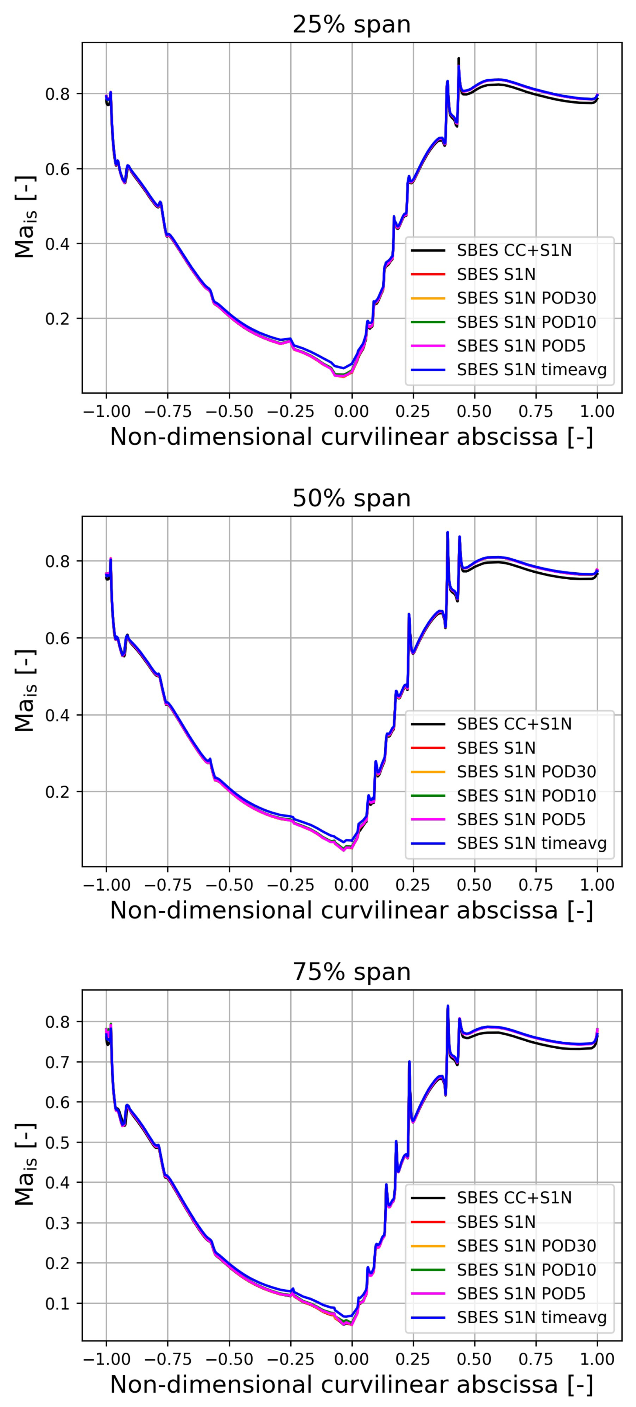
In order to better compare the decoupled simulations with the coupled one, Figure 15 reports the vane loads in terms of isentropic Mach number at 25%, 50%, and 75% of the span for all the simulations. The isentropic Mach number is reported as a function of the non-dimensional curvilinear abscissa, whose negative values are associated with the pressure side and positive ones with the suction side. As can be noted from the figure, the isentropic Mach number distributions of all the decoupled simulations fall very close to that of the SBES CC+S1N calculation. This confirms that the boundary conditions at the S1N inlet for all the decoupled cases are correctly imposed and that they are able to correctly retrieve the S1N aerothermal field.

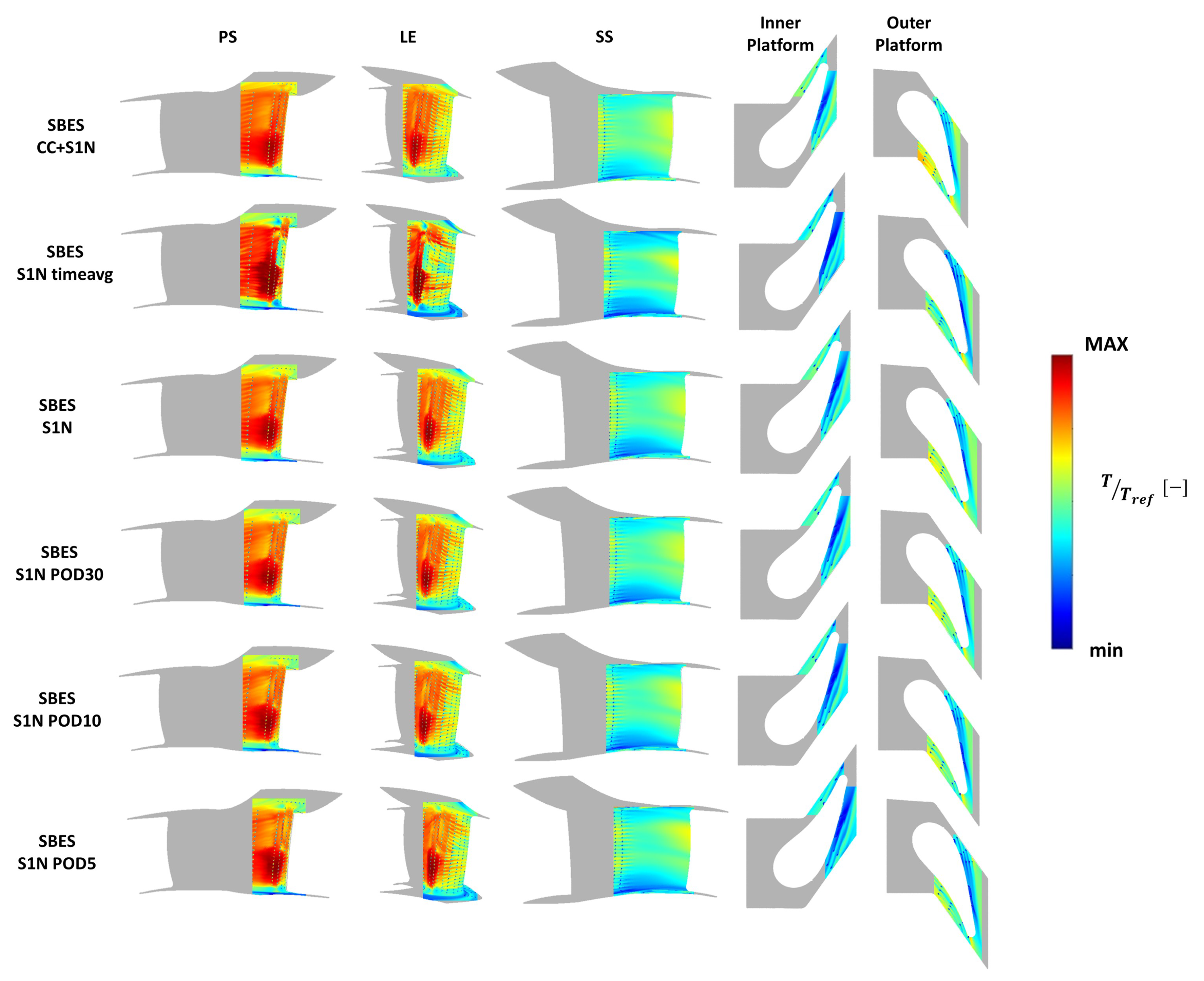
However, on the contrary, more relevant discrepancies between the numerical calculations are observable by looking at the prediction of the static temperature distribution along the stator. In this regard, Figure 16 reports the normalized static temperature distribution over the vane surface, including the endwalls, for all SBES calculations. Focusing firstly on the SBES S1N timeavg and SBES S1N, evident discrepancies can be noted between the two cases. As a matter of fact, from the 2D maps, it is clear that the SBES S1N case is extremely similar to the starting case SBES CC+S1N, both on the LE and on the PS and SS. On the contrary, applying average and constant conditions over time to the stator inlet leads to obvious errors in the prediction of the wall temperature distribution. In fact, focusing on the PS, it is possible to notice a considerable overestimation of the wall temperature on the lower part of the PS. Similarly, even on the upper part of the PS, a similar behavior can be seen, albeit less accentuated than for the lower part. On the SS, on the other hand, the differences are less marked, although at around 50% of the span, a greater coverage by the coolant is evident, resulting in a less homogeneous temperature distribution compared to SBES CC+S1N. Even greater differences can be noted on the LE, where the wall temperature predicted by SBES S1N timeavg is highly non-uniform, with it being evident that a non-negligible portion of the LE is left completely uncovered by the cooling system while at around 50% of the span the temperature prediction is clearly underestimated.

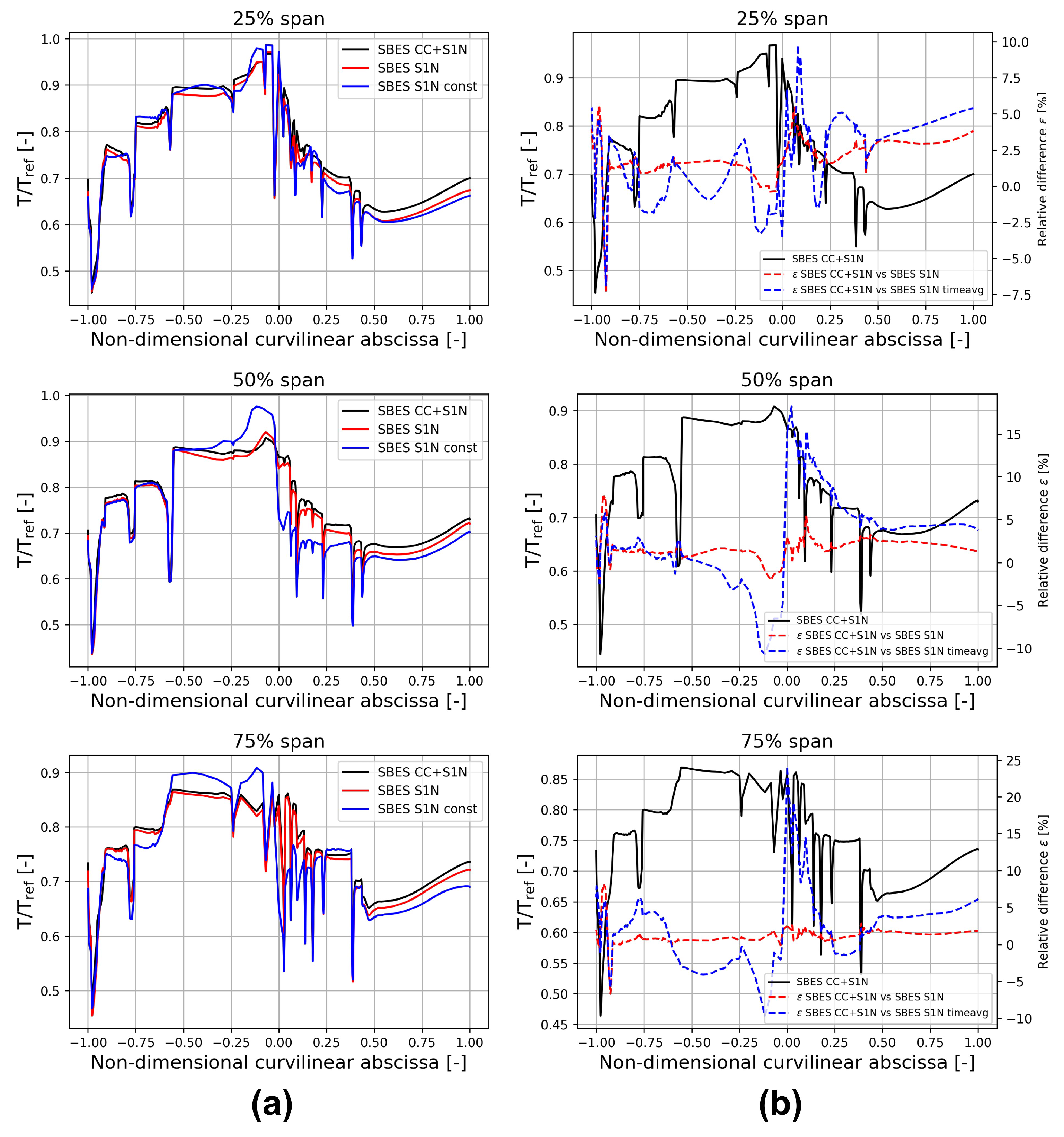
Moreover, in order to better quantify the differences between the simulations, Figure 17 shows the relative differences, in terms of normalized temperature distribution, between SBES S1N (in red) and SBES S1N timeavg (in blue) with respect to the temperature profile of the case SBES CC+S1N (in black) at 25%, 50%, and 75% of the span.

As can be seen, for the SBES S1N case the relative error is always contained within 5% for all the span values considered, with the exception of some points on the PS around the TE, where the slot cooling system is present. Hence, SBES S1N tends to predict a temperature distribution very similar to the reference case SBES CC+S1N for all span values considered. For the SBES S1N timeavg simulation, on the other hand, the differences are consistent for all three span values: in particular, generally speaking, the greatest deviation is present around the LE, an area characterized as seen by an extremely uneven wall temperature destruction, reaching peaks in the relative error corresponding approximately to 10%, 20%, and 25%, respectively, at 25%, 50%, and 75% of the span. In particular, focusing on 50% of the span, an overestimation of the temperature around the LE PS side is evident, already extremely evident from the 2D maps, while a non-negligible temperature underestimation is present on the SS side, in correspondence to which a greater non-homogeneity in the contour temperature had been highlighted in the corresponding 2D map. In the same way, a very similar behavior for the SBES S1N timeavg simulation can also be observed at 75% of the span, where also on the PS, for a curvilinear abscissa greater than −0.5, an underestimated prediction of the wall temperature is evident. In conclusion, applying constant and time-averaged conditions leads to non-negligible inaccuracies in the prediction of the temperature distribution on the blade, especially on the LE, although the average values applied on the stator inlet correspond to those of the SBES CC+S1N and SBES S1N. This further confirms the need to generate realistic and representative conditions to carry out decoupled simulations of the S1N alone.

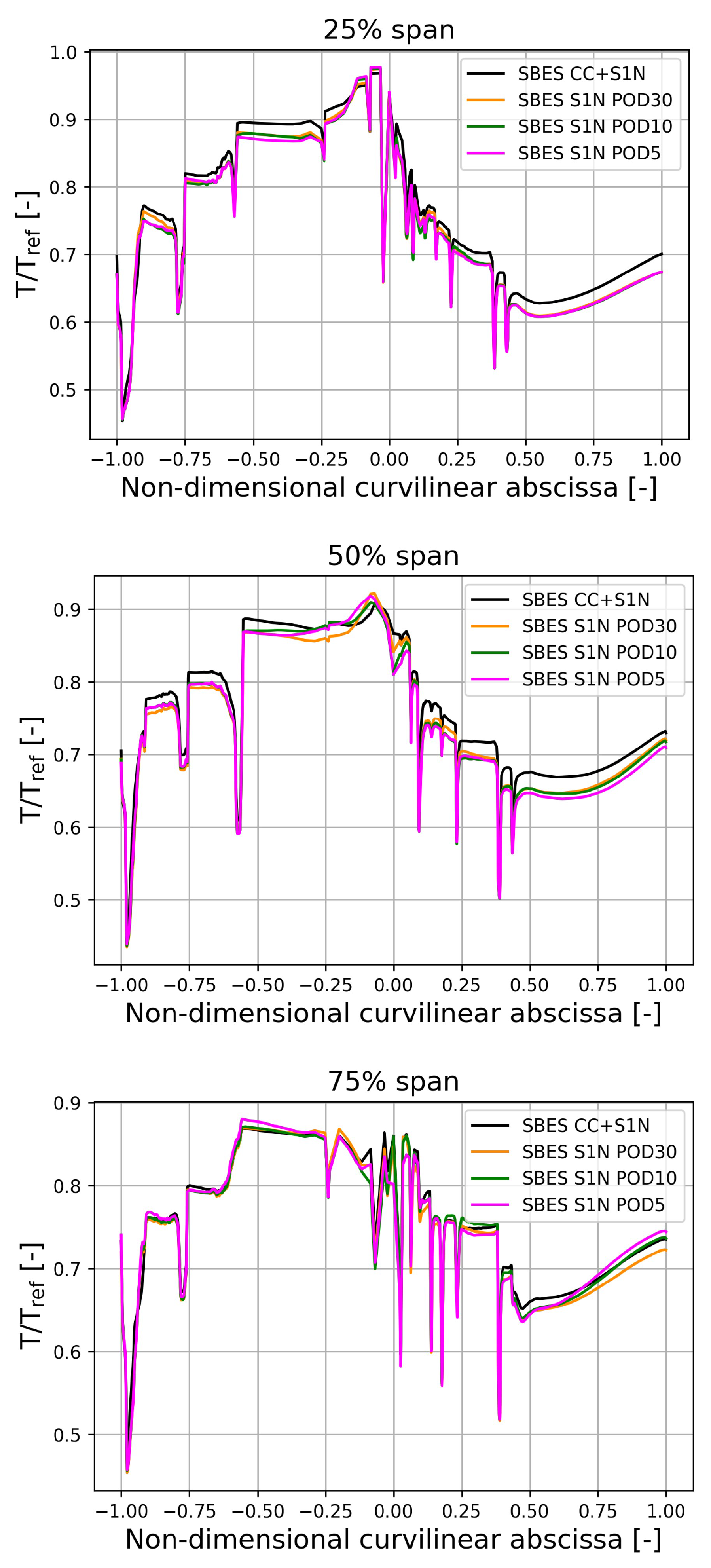
Focusing now on the 2D maps related to the application of the POD technique considering the first 30 modes (SBES S1N POD30), the first 10 (SBES S1N POD10), and the first 5 (SBES S1N POD5), it is possible to observe that the contours are in all cases very similar to the fully integrated simulation. Similar considerations can also be applied to the inner and outer platforms, where again there is a good match with respect to the SBES CC+S1N. However, the contours, especially on the PS and LE, indicate that considering fewer POD modes leads to a slightly more uneven wall temperature distribution. This behavior can be explained by taking into account that fewer POD modes correspond to lower energy content considered at the stator inlet. The same phenomena can be also observed in the 1D radial profiles. In order to go into more details about the temperature distribution, the 1D profiles of the normalized wall temperature over the vane are also reported in Figure 18 as a function of the non-dimensional curvilinear abscissa for the SBES CC+S1N, SBES S1N POD30, SBES S1N POD10, and SBES S1N POD5 calculations. As can be seen, the wall temperature predictions for all the simulations fall very close to the SBES CC+S1N case, bringing them to a very satisfactory match. This observation implies that the application of the POD technique leads to satisfactory results and that the main coherent structures that contribute most to the dynamics of the system have been correctly identified by the POD modes, confirming once again that this technique can be used to characterize the phenomena related to combustor–turbine interactions.

7.6. Analysis of the Plane Outlet Conditions

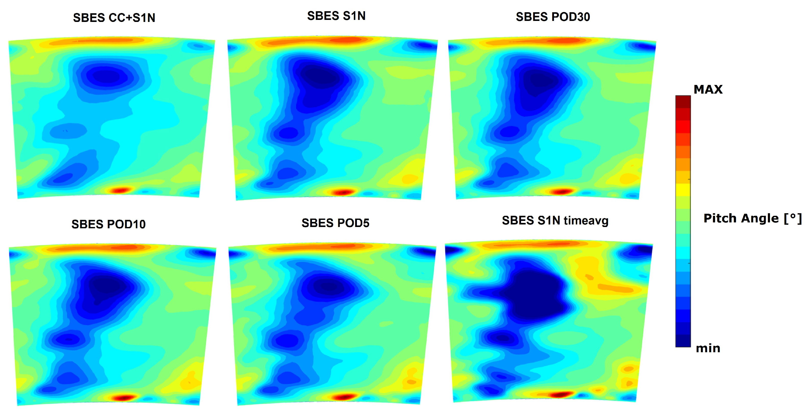
In order to highlight the differences between a fully integrated simulation and decoupled ones, an analysis of the outlet plane conditions is also reported, since they can the affect lifetime and the performance of the following rotor. Firstly, Figure 19 and Figure 20 report the two-dimensional maps of pitch and swirl angle, defined according to Equations (16) and (17), at the stator outlet for all the simulations. As can be seen, both the swirl and pitch distributions are comparable between all the SBES simulations, confirming the accuracy of the set of inlet boundary conditions applied for all the decoupled simulations. As can be noted from the figures, the swirl and pitch distributions of the stand-alone S1N simulations are quite similar to the fully integrated ones. However, despite the trends being comparable, some discrepancies can be still found, especially in correspondence of the wake. In particular, looking at the S1N SBES timeavg contours, it is evident that the pitch distribution does not perfectly match the data from the fully integrated SBES simulation, predicting a more intense and dishomogeneous distribution, especially from 70% of the span, where a region characterized by higher pitch values can be found only in this case. The same phenomena can be also noted, especially from 50% to 70% of the span, by looking at Figure 21, where the corresponding 1D radial profile is reported. Moreover, all the decoupled simulations share a slight overestimation of the pitch angle around 10% of the span.

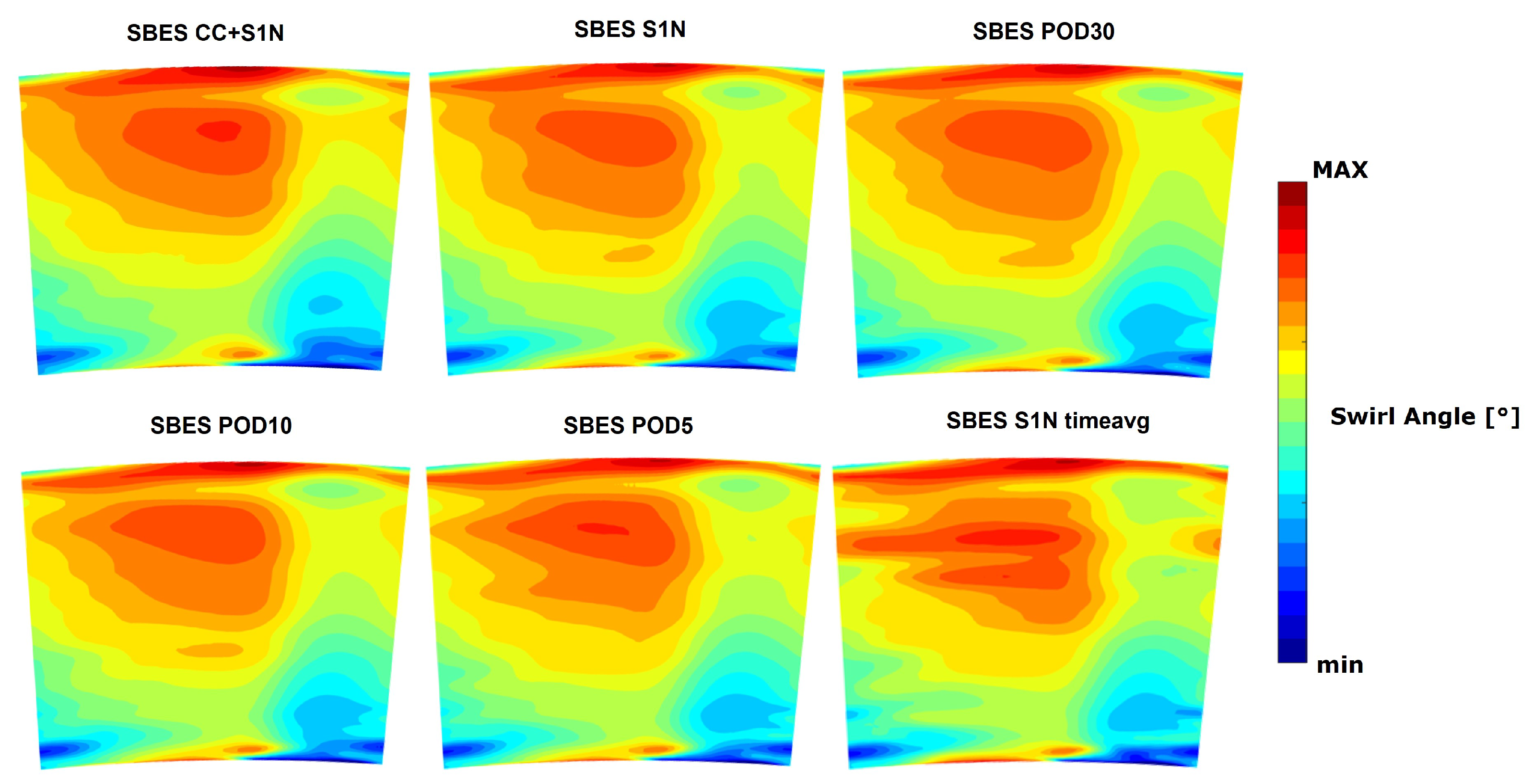
A similar reasoning can also be applied to the swirl angle. In this case too, applying time-averaged boundary conditions at the stator inlet leads to a more intense and dishomogeneous distribution in terms of the two-dimensional map, as can be seen from Figure 20. This discrepancy results in a less constant swirl distribution between 70% and 90% of the span, as can be seen from Figure 21, where the corresponding 1D radial profiles are reported for all the simulations. Furthermore, in this case, especially near the hub region, approximately until 10% of the span, a deviation from the coupled SBES solution can be observed. However, in conclusion, for all the simulations, especially for the ones where time-varying boundary conditions are imposed, the pitch and swirl angle distributions fall very close to the coupled simulation, bringing a very satisfactory match.

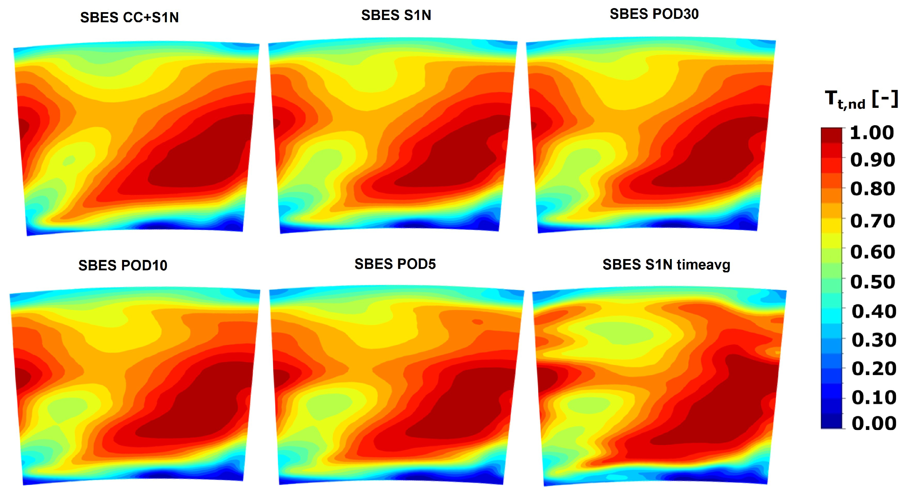
Moreover, the contours of normalized total temperature, according to Equation (15), extracted at the outlet plane are reported in Figure 22 for all the SBES simulations. As can be seen, all the 2D maps present a very similar distribution, especially for all the stand-alone S1N SBES calculations, with the exception of SBES S1N timeavg one. As a matter of fact, similarly to the pitch and swirl angles, also in this case, the 2D contour of the SBES S1N timeavg is characterized by a more distorted distribution, especially in correspondence of the wake, from 60% of the span. However, these discrepancies are not so evident by looking at the averaged 1D radial profiles, as reported in Figure 21.

In conclusion, from the analysis of the outlet plane, on the whole, only slight differences emerge between the stand-alone S1N SBES calculations and the fully integrated one, with the only exception being the SBES S1N timeavg calculation. Hence, taking as a reference the SBES CC+S1N case, imposing time-varying boundary conditions at the inlet of the S1N, taking into account the effect of the unsteadiness, provides more reliable and accurate results in terms of 2D quantity distributions at the outlet plane. This consideration can be extended also to the SBES S1N simulations where the POD technique has been employed (SBES S1N 30POD, SBES S1N 10POD, and SBES S1N 5POD), demonstrating that including only the first five POD modes, corresponding to 30% of the total energy, leads to satisfactory accurate results.

8. Conclusions

In conclusion, the purpose of the present work is to compare a fully integrated combustor–stator (SBES CC+S1N) SBES simulation and isolated stator SBES simulations. To achieve this, the fully unsteady inlet condition of the stator has been recorded and reconstructed at the interface plane between the two components from the fully integrated SBES. Firstly, recorded snapshots are employed to recreate more realistic and as representative as possible unsteady boundary conditions without any further post-processing operation (SBES S1N). Then, the proper orthogonal decomposition (POD) technique has been applied taking into account three different number of POD modes (30, 10, 5) corresponding to a descending level of energy content (80%, 50%, 30%) with respect to the global turbulent kinetic energy (SBES S1N POD30, SBES S1N POD10, SBES S1N POD5). The results have then been compared to an SBES of the stand-alone stator obtained by imposing time-averaged 2D maps from the fully integrated SBES simulation (SBES S1N timeavg). In order to investigate the interaction between the combustor and the first-stage nozzle, numerical simulations are carried out under realistic operating conditions and geometry. As a matter of fact, the interaction between the main hot flow from the combustor and the cooling flows is studied by including a realistic turbine nozzle cooling system. Hence, all the SBES simulations of the isolated stator have been performed with the aim of determining whether the flow field obtained is comparable with that of the integrated simulation, assumed as a reference, allowing more realistic results to be obtained rather than imposing time-averaged 2D maps, as per standard design practice.

Firstly, the focus lies on the ability of time-varying boundary conditions to reconstruct the flow field at the interface plane between the combustor and turbine compared to the integrated simulation. To achieve this, the RMS U_x, RMS U_y, RMS U_z, and RMS T_t for S1N SBES and S1N timeavg calculations are compared with SBES CC+S1N, selected as a reference. Looking at the results, it is possible to conclude that the applied time-varying boundary conditions are able to successfully replicate the turbulence kinetic energy at the inlet of the stator, contrary to what happens with constant boundary conditions (SBES timeavg).

Then, after presenting an analysis of sensitivity for the definition of the number of snapshots, the POD technique has been applied, taking into account three different numbers of POD modes. To better understand the coherent structures that can be identified by the POD modes, the most relevant information about the $\rho u_x$ and normalized total temperature in terms of both spatial and temporal modes for the first three coherent structures have been studied. In addition to showing a remarkable blockage effect due to the presence of the stator, the contours showed that greater levels of turbulence and flow unsteadiness effects are mainly concentrated in these regions, caused by the presence of the outgoing flow from the nuggets.

In order to better compare the decoupled simulations with the coupled one, the total temperature RMS distribution for all the decoupled simulations and for the coupled simulation, taken as a reference, are studied at the interface plane between the combustor and turbine. From the results, it can be observed that as the number of POD modes considered decreases, the RMS values become increasingly lower, as expected, as can be well observed above all from the SBES S1N 5POD simulation.

Moreover, looking at the normalized static temperature 2D distribution over the vane surface for all SBES calculations, it is clear that the isolated S1N simulations, where unsteady boundary conditions are applied, are very similar to the SBES CC+S1N simulation, both on the LE and on the PS and SS. On the contrary, applying average and constant conditions over time to the stator inlet leads to obvious errors in the prediction of the wall temperature distribution, especially on PS and LE.

Then, an analysis of the outlet plane conditions is reported, focusing on the pitch and swirl angles and the normalized total temperature. In this case, the results show that the distributions are comparable between all the SBES simulations, confirming the accuracy of the set of inlet boundary conditions applied for all the decoupled simulations. However, despite the trends being comparable, some discrepancies can be still found, especially in correspondence of the wake, looking at the S1N SBES timeavg simulation.

In conclusion, it is possible to conclude that, taking as reference a coupled simulation, imposing time-varying boundary conditions at the inlet of the S1N taking into account the effect of the unsteadiness provides more reliable and accurate results in terms of 2D quantity distributions at the outlet plane. This consideration can be extended also to the SBES S1N simulations where the POD technique has been employed (SBES S1N 30POD, SBES S1N 10POD, and SBES S1N 5POD), demonstrating that including only the first five POD modes, corresponding to 30% of the total energy, leads to satisfactorily accurate results.