Finite Time Disturbance Observer Based on Air Conditioning System Control Scheme

Abstract

A novel robust finite time disturbance observer (RFTDO) based on an independent output-finite time composite control (FTCC) scheme is proposed for an air conditioning-system temperature and humidity regulation. The variable air volume (VAV) of the system is represented by two first-order mathematical models for the temperature and humidity dynamics. In the temperature loop dynamics, a RFTDO temperature (RFTDO-T) and an FTCC temperature (FTCC-T) are designed to estimate and reject the lumped disturbances of the temperature subsystem. In the humidity loop, a robust output of the FTCC humidity (FTCC-H) and RFTDO humidity (RFTDO-H) are also designed to estimate and reject the lumped disturbances of the humidity subsystem. Based on Lyapunov theory, the stability proof of the two closed-loop controllers and observers is presented. Comparative simulations are carried out to confirm that the proposed controller outperforms conventional methods and offers greater accuracy of temperature, humidity, and carbon dioxide concentration, having superior regulation performance in terms of a rapid finite time convergence, an outstanding disturbance rejection property, and better energy consumption. In addition to presenting the comparative simulation results from the control applications on the VAV system, the quantitative values are provided to further confirm the superiority of the proposed controller. In particular, the proposed method exhibits the shortest settling time of, respectively, 15 and 40 min to reach the expected temperature and humidity, whereas other comparative controllers require a longer time to settle down.

1. Introduction

Demand for effective indoor air quality and climate control for heating, ventilating, and air conditioning (HVAC) systems in commercial buildings accounts for approximately 70–90% of the building’s energy consumption [1,2]. Commercial energy consumption entails a significant “carbon footprint”, or contribution to global emissions which exacerbate climate change, and many businesses are committed to minimizing their environmental impact [3,4]. Consequently, there is significant demand for effective energy consumption management systems to maintain good indoor air quality, achieve acceptable thermal comfort, and minimize energy usage and wastage.

Current research is focused on developing robust HVAC control systems to achieve acceptability of parameters such as temperature, humidity, and carbon dioxide concentration. Several control schemes have been embedded in HVAC systems, such as proportional–integral–derivative (PID) control [5,6], sliding mode control (SMC) schemes [7,8,9,10], model predictive control (MPC) [11,12,13,14], feedback linearization [15,16,17], etc. In addition, the operating environment of the HVAC system presents uncertainties and disturbances which impact on controller performance, such as air supply fluctuation, parametric uncertainties, unmodeled dynamics, and time delays, which deteriorate the tracking and regulation performance. Thus, it is necessary to consider the disturbance compensation and active rejection in the HVAC control design to accomplish satisfactory control performance. In the existing literature of the temperature control, the disturbance compensation-based control has been proposed for different system applications [11,12,13,14,15,16,17]. However, those systems have only one variable to be controlled, while the HVAC systems at least could have multivariable of temperature, humidity, and CO₂ which are required to be controller simultaneously.

Standard HVAC control systems for temperature and relative humidity are based on multiloop PID control [5,6]. Castilla et al. [11] suggested complex regulation procedures to maintain acceptable thermal comfort conditions in confined environments based on the `users’ productivity and an indirect effect on energy saving. Complex regulation uses a non-linear model predictive controller to maintain high thermal comfort levels whilst reducing energy consumption.

In an HVAC system consisting of multiple air handling units with variable air volume units, Kalaimani et al. [18] presented a controller based on several personal thermal comfort systems, which they called “SPOT”, using model predictive control (MPC). This controller combined a two-time-scale MPC-based predictive controller for the HVAC system (at the 1 h and 10-min time scales) using a non-linear thermal model with reactive control by the SPOT systems at the fastest (30 s) time scale. Their controller achieved 45% and 15% savings of energy in summer and winter, respectively. Alamin et al. [12] presented an MPC controller to calculate how much money it costs for the required energy to reach the desired thermal comfort associated with the HVAC. This was based on optimizing the fan coil speed to achieve an acceptable thermal comfort satisfaction. The temperature and relative humidity independent control system to ensure energy saving has been in the interest of researchers in the last decade [19,20]. These researchers focused on improving indoor air quality and thermal comfort parameters using a dehumidification system embedded in an HVAC system [21,22,23,24]. These studies focus on developing different controllers for the temperature or the humidity. Attia et al. [23] compared fuzzy logic control to the PID control in residential buildings to control the temperature and relative humidity during partial and complete load in different climates. These techniques were proposed to maintain the targeted temperature and relative humidity in the dwelling using an HVAC system with the main focus on reducing energy consumption presented as the electrical intake from the HVAC compressor [24].

In addition, many applications of model predictive control (MPC) for HVAC systems have been reported in the existing literature [25,26,27,28,29,30,31]. In [25], a stability margin and gap metric based on a reduced multiple-MPC is proposed for the nonlinear HVAC. In [26], an optimal energy management strategy based on a nonlinear predictive model is presented for a plant of a test building within a single-zone by using singular perturbation arguments to introduce a multiple time scale dynamic response of buildings with energy recovery. In addition, a distributed MPC scheme is presented in [27] for regulating building temperature with a single zone building a multi-zone. In [28], the MPC with time-varying constraints framework is designed for building climate control in the presence of parametric uncertainties, in which linear matrix inequalities are used for optimization problems. In [29], the predictive control based on the number of occupants detected by video data is proposed for an indoor environment incorporating CO₂ concentration measures. In [30], a MPC is developed for an air-conditioning system with a dedicated outdoor air system, in which a linear building model is employed to optimize indoor comfort and energy use, and a lecture theatre for real-time control is used to experimentally demonstrate the system. In [31], a nonlinear MPC (NMPC) approach is implemented for the HVAC system that is modelled by index-1 differential-algebraic equations, derived from energy balances and rigorous material. However, the primary shortcoming of model predictive control schemes is that the control algorithms largely rely on a precise system model that is crucial to the prediction stage. As a result, any non-exact cancellation in the dynamic model severely affects the closed-loop controlled system performance.

In this paper, we propose a finite time composite control (FTCC) method that is effective and robust for an application to an air conditioning system. We will present a new design of robust finite time disturbance observer (RFTDO) technique-based output feedback FTCC, which attenuates the influence of system uncertainties and disturbances on the system humidity, temperature, and carbon dioxide outputs. The aim of the proposed control scheme is to effectively regulate humidity and temperature outputs to ensure that they converge to their corresponding references in finite time, whilst also maintaining the robustness of control action. The following lists the significant contributions made in this paper:

(1) By using a nonlinear function in the finite time disturbance observer (FTDO), a novel robust FTDO (RFTDO) is designed for the HVAC system to enhance the disturbance estimation effectiveness. Accordingly, two RFTDO temperature (RFTDO-T) and humidity (RFTDO-H) estimators are proposed to estimate the lumped disturbances acting on the temperature and humidity subsystems of the HVAC, respectively. Then, the rigorous stability and convergence analysis of the proposed RFTDO is performed. This constitutes an improvement to both the disturbance estimation and the finite time convergence. The state of the art in the RFTDO-T and RFTDO-H estimators proposed for the temperature and humidity subsystem, respectively, is centered on not only ensuring the finite time convergence of estimations, but also enhancing the robustness property.

(2) Then, the estimations of the lumped disturbances information are used to reject these disturbances during the design procedure of FTCC. Under the independent control structure; by integrating the lumped disturbance estimations in the temperature and humidity controller, the FTCC temperature (FTCC-T) and FTCC humidity (FTCC-H) schemes are proposed to improve the temperature and humidity regulation precision.

(3) Not only the disturbance estimation enhancement and control robustness are guaranteed, but also the finite time convergence of the control and observer element of both the FTCC-T and FTCC-H is ensured. Thus, the temperature and humidity output of the HVAC system are regulated to their desired values at the finite time.

(4) Finally, simulation results are presented to verify the superiority of the proposed temperature and humidity control approach compared with composite linear control, the ADRC, and SMC.

2. The State of the Art of the Work

In this section, a state-of-the-art review of the estimators used in this work is presented and the contribution of this paper is clarified, with respect to the proposed estimator. In the literature, there have been many attempts at applying observer techniques to HVAC systems to cope with the issue of temperature and humidity states and the overall disturbance estimation. For instance, in [32], minimum-order and full-order observers are proposed for the air handling units with system uncertainties to estimate online the state variables of indoor temperature and relative humidity. Moreover, a regulator system for disturbance rejection is designed using the Lyapunov stability theory. In [33], a load disturbance observer is designed for estimation of non-measurable heat and moisture load disturbances that can be completely compensated by a backstepping controller applied to the HVAC system linearized model in the presence of time-varying loads. In [34], the stochastic grey-box modelling approach is proposed for estimating the ventilation air change rate of a room, which can assist in overcoming disturbances acting on the indoor room system. However, the convergence rate of estimations to their corresponding true values is asymptotic. This means that the estimation errors of both disturbances and the system states converge to zero slowly, and the estimation accuracy by the above observers is limited. To speed up the estimation error convergence, the finite time observers were proposed by [35], which have been successfully applied in many applications such as electric furnace and robot systems [36,37], electronic throttle systems [38,39], dc–dc buck converters [40], dc servomotors [41], etc.

Most of the observation techniques for HVAC systems that appeared in the literature have certain issues that need attention. First, many of them ensure asymptotic and slow estimation of all state variables and disturbances. Next, those observers frequently lack robustness against the first-order time derivative of the total lumped disturbance and uncertainties. Moreover, some estimate the system state variables and disturbances in a separated manner. After a review of the state-of-the-art of the estimators applied to the HVAC systems above, we propose a novel robust finite-time disturbance observer for the temperature loop denoted by the RFTDO-T estimator and for the humidity loop denoted by the RFTDO-H estimator. The reasons for using those estimators are to estimate the disturbance in a finite time. With the assistance of the disturbance estimation, the output response of temperature and humidity of the HVAC is free from an offset and deviation caused by such disturbances. Compared to the state of the art in designing disturbance estimators, the primary contribution of the estimator designs in the current paper is that the robustness of both RFTDO-T and RFTDO-H is enhanced by incorporating the nonlinear function terms. In addition, the finite time stability of these estimators under the robustness terms is newly analyzed by using the Lyapunov theorem. Moreover, since there are fewer results from applying observers, the current work will pave the way for more facile applications of different types of observers to the HVAC systems.

3. Mathematical Modeling of Air Conditioning System

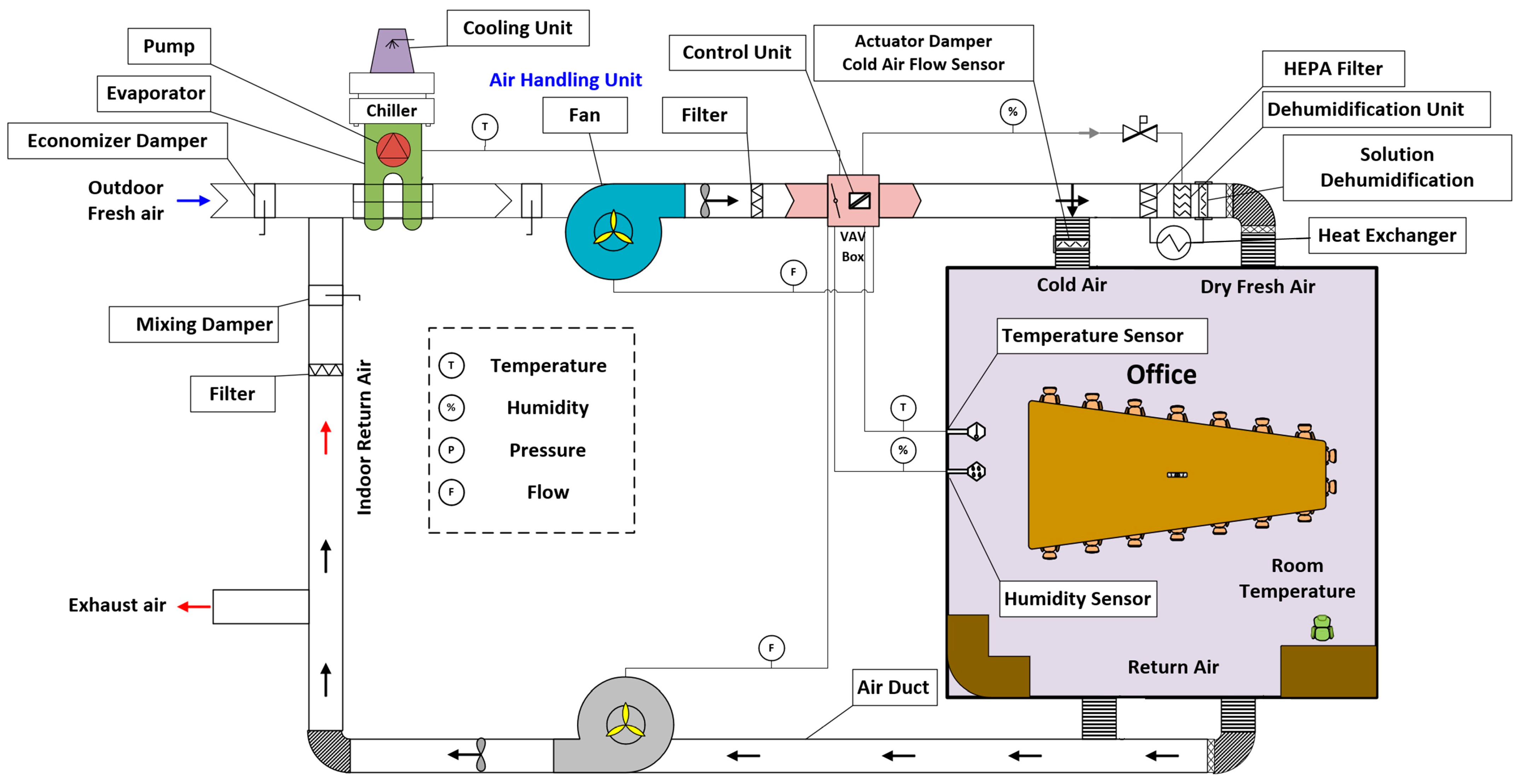
The architecture of the air-conditioning system is illustrated in Figure 1, and its basic components are described as follows. It mainly consists of an air handling unit, air supply pipeline module, indoor air supply terminal, electric control unit, and a common all-air module. First, the outdoor fresh air and the indoor return air are mixed. Second, the mixed air is chilled and sent to each room. Figure 1 shows the schematic diagram of an independent control unit for temperature and relative humidity, using a chiller, based on the variable air volume (VAV) method of fresh air supply by the dehumidification unit (HEPA filter, heat exchanger, dehumidifier) and the fresh cool air supplied by the temperature control unit. The device works to achieve thermal comfort and air quality parameters, adjusting (reducing or increasing) the temperature, relative humidity, and filtering particulate matters in the office. A robust feedback controller adjusts the supply fan speed and heat exchanger settings to target the setpoint temperature. The return fan includes a HEPA filter and a flow controller, which targets the airflow rate to a particular setpoint. The outdoor air controller regulates the positions of the mixing damper, outdoor air damper and exhaust damper to control the outdoor air ratio. The purpose of this is to sustain a positive pressure and moderate airflow. In this study, the mathematical model is solved based on the assumptions: (i) the office room is closed-system, sealed by way of double-glazed windows and automatic doors; (ii) based on (i), the change in air pressure is equal to zero; (iii) the indoor temperature is measured using sensors and with the objective of achieving desirable fresh air diffusion; (iv) the changes in the indoor relative humidity are impacted by many factors such as the number of occupants and activities which create humidity (for example, steam from using the office kitchen facilities), which will affect the office room temperature.

The air-conditioning system dynamics can be described by a standard temperature model and a humidity dynamic model. The plant system parameters and their nominal values are listed in

Table 1. System parameters values.

Descriptions	Parameters	Nominal Values
Wall area	$F \left[{\mathrm{m}}^2\right]$	208
Wall material thermal conductivity	$\lambda$ $\left[ \mathrm{W}/\left(\mathrm{mK}\right)\right]$	0.58
Wall material thickness	$\delta \left[\mathrm{m}\right]$	0.5
Glass window (inner wall) heat transfer coefficient	${\alpha }_i$[$\mathrm{W}/\left({\mathrm{m}}^2\mathrm{K}\right)]$	5.6
Air density (indoor)	$\rho \left[\frac{\mathrm{kg}}{{\mathrm{m}}^3}\right]$	1.204
Volume of the room	$V \left[{\mathrm{m}}^3\right]$	16 × 10 × 4
Air specific heat capacity (indoor)	$C_1\left[\frac{\mathrm{kJ}}{\mathrm{kg}*\mathrm{K}}\right]$	1.003
Total mass of air in building	$M_n\left[\mathrm{g}\right]$	768,000
Number of room occupants	$n$	10
Cluster coefficient for room occupants	$\varphi$	0.95
Quantity of moisture dissipated by room occupants	$\mathrm{g}\left[\frac{\mathrm{g}}{\mathrm{h}}\right]$	1000
Infiltration air volume	$L \left[{\mathrm{m}}^3\right]$	268

. The overall system dynamics that comprise dynamic response of temperature and humidity subsystem [9] can be expressed as

$${\dot{x}}_1\left(t\right)=-\left[\frac{F\lambda }{\rho V{C}_1\delta }+\frac{{\alpha }_i}{\rho V{C}_1}\right]\left(T_o\left(t\right)-T_s+x_1\left(t\right)\right)-\frac{1}{\rho V{C}_1}\sigma \left(t\right)-\frac{1}{V}{u}_1\left(t\right)$$

(1)

$${\dot{x}}_2\left(t\right)=-\frac{L\rho }{M_n}\left(d_o\left(t\right)-d_s+x_2\left(t\right)\right)-\frac{0.27n\varnothing g*{10}^{-6}}{M_n}-\frac{1}{M_n}{u}_2\left(t\right)$$

(2)

with

$$x_1\left(t\right)=T_s-T_i\left(t\right), x_2\left(t\right)=d_s-d_n\left(t\right)$$

$$u_1\left(t\right)=G_s\left(T_s-T_i\left(t\right)\right), u_2\left(t\right)=G_o\left(d_s-d_n\left(t\right)\right)$$

where $T_i$; T_s, and T_o are the room, the dry fan coil (sensible heat), and the outdoor ambient temperature $(℃),$respectively. $d_n\left(t\right)$ represents the building air’s moisture content $\left(\mathrm{g}/\mathrm{kg}\right)$; $d_s$ is the moisture content of the air conditioner’s supplied air $\left(\mathrm{g}/\mathrm{kg}\right)$; and $d_o$ is the outdoor air’s moisture content $\left(\mathrm{g}/\mathrm{kg}\right)$. Equation (1) is based on the heat energy balance in an air-conditioning system in which $\left[\frac{F\lambda }{\rho V{C}_1\delta }+\frac{{\alpha }_i}{\rho V{C}_1}\right]\left(T_o\left(t\right)-T_s+x_1\left(t\right)\right)$ represents the heat provided by the cooling coil, and the heat dissipation, respectively, and $\frac{1}{\rho V{C}_1}\sigma \left(t\right)$ refers to the heat radiation of the room window glass generated by sun. This equation will be controlled using $u_1\left(t\right)$ as an input temperature. Equation (2) is based on the mass conservation of air humidity with the assumption that the office is a closed-loop system and the pressure in the commercial building is constant, in which $\frac{L\rho }{M_n}\left(d_o\left(t\right)-d_s+x_2\left(t\right)\right)$ represents the wet load due to the fresh air penetration and $\frac{0.27n\varnothing g}{M_n}$ is the wet load of personnel. This equation will be controlled using $u_2\left(t\right)$ as an input humidity. $u_1\left(t\right)$ and $u_2\left(t\right)$ are actuated by the air supply volume using two dampers for the cold air flow and for the dehumidified air as shown in Figure 1 relying on $G_s$ (heat removal air supply) and $G_o$ (exhaust volume of the dehumidification) [42].

Such control inputs will be designed by our controllers to supply the required air temperature and humidity as well as meeting the occupants’ requirements for thermal comfort.

Based on Equations (1) and (2), the air conditioner system dynamics can be written in the following state space form

$${\dot{x}}_1\left(t\right)=f_1\left(x_1, t\right)+b_1{u}_1\left(t\right)+d_1\left(t\right)$$

(3)

$${\dot{x}}_2\left(t\right)=f_2\left(x_2, t\right)+b_2{u}_2\left(t\right)+d_2\left(t\right)$$

(4)

where

$$f_1\left(x_1,t\right)=-\left[\frac{F\lambda }{\rho V{C}_1\delta }+\frac{{\alpha }_i}{\rho V{C}_1}\right]\left(T_o\left(t\right)-T_s+x_1\left(t\right)\right)-\frac{1}{\rho V{C}_1}\sigma \left(t\right)$$

$$b_1=-\frac{1}{V}$$

$$f_2\left(x_2,t\right)=-\frac{L\rho }{M_n}\left(d_o\left(t\right)-d_s+x_2\left(t\right)\right)-\frac{0.27n\varnothing g*{10}^{-6}}{M_n}$$

$$b_2=-\frac{1}{M_n}$$

where $d_1\left(t\right)$ and $d_2\left(t\right)$ represent external disturbances acting on the temperature and humidity subsystem. It must be noted that the system functions $f_1\left(x_1,t\right)$ and $f_2\left(x_2,t\right)$, and the input coefficients $b_1$ and $b_2$ cannot be exactly known due to system uncertainties and hence have to be expressed as $f_i\left(x_i,t\right)$ = $f_{0i}\left(x_i,t\right)+\Delta f_i\left(x_i,t\right)$ for $i=1, 2$ and $b_i=b_{oi}+\Delta b_i$ for $i=1, 2$ where $f_{0i}$ and $b_{oi}$ are the nominal parts of $f_{ }\left(x_i,t\right)$ and $b_i$.

$\Delta f_i\left(x_i,t\right)$ and $\Delta b_i$ represent modeling errors and are presumed to be differential with respect to time. Generally, the state space form of Equations (3) and (4) can be rewritten as

$${\dot{x}}_i\left(t\right)=f_{0i}\left(x_i, t\right)+\Delta f_i\left(x_i,t\right)+\left(b_{0i}+\Delta b_i\right)u_i\left(t\right)+d_i\left(t\right) \mathrm{for} i=1,2.$$

(5)

The term

$$D_i\left(x_i,d_i,t\right)=f_{0i}\left(x_i, t\right)+\Delta f_i\left(x_i,t\right)+\Delta b_i{u}_i\left(t\right)+d_i \mathrm{for} i=1,2.$$

(6)

is considered to be equivalent to the lumped disturbance. Thus, the state space representation (5) used for further analysis is

$${\dot{x}}_i\left(t\right)=D\left(x_i,d_i,t\right)+b_{0i}{u}_i\left(t\right) \mathrm{for} i=1,2.$$

(7)

Hence, the control objective is to design a constructive control strategy for the system dynamics given in (7) such that an accurate temperature and humidity regulation can be attained in a finite time regardless of system uncertainties and external disturbances. Mathematically, the objective can be expressed as

$$\underset{t\to t_{f1}}{\lim }{T}_i=T_d, \underset{t\to t_{f2}}{\lim }{d}_n=d_l$$

(8)

where $T_d$ and $d_l$ are the desired temperature and humidity, respectively, which are pre-adjusted to meet satisfactory thermal comfort parameters in the room environment. Furthermore, $t_{f1}$ and $t_{f2}$ are the finite times when the actual outputs of the HVAC of $T_i$ and $d_n$ converge to the references of $T_d$ and $d_l$, respectively.

4. Proposed Control Design for the Air Conditioning System

Based on the literature [42,43,44,45,46], the air-conditioning systems consists of one air handling unit (AHU) which supplies air to VAV terminals using the supply and return fans and the VAV system which is cooled by chilled water coming from the AHU coil. Therefore, the desired condition within the system is regulated by local controllers. This will result in the current PID temperature controller maintaining the desired room temperature. Depending on the air mixture and after the filter, the outside air is cooled by the chiller and the outside air is dehumidified by the dehumidification solution and then supplied to the room by the supply fan. However, to adjust the humidity, the temperature will change as well (and vice versa) so it is recommended by [44] to introduce two controllers with a self-turning parameter for two feedback control loops of temperature and Humidity with CO₂ as subsystems. Therefore, the decoupling control principal is recommended by the literature when it is difficult to avoid the impact of the temperature on the dehumidification process for complex systems in commercial buildings [46], this concept was validated experimentally by [42]. 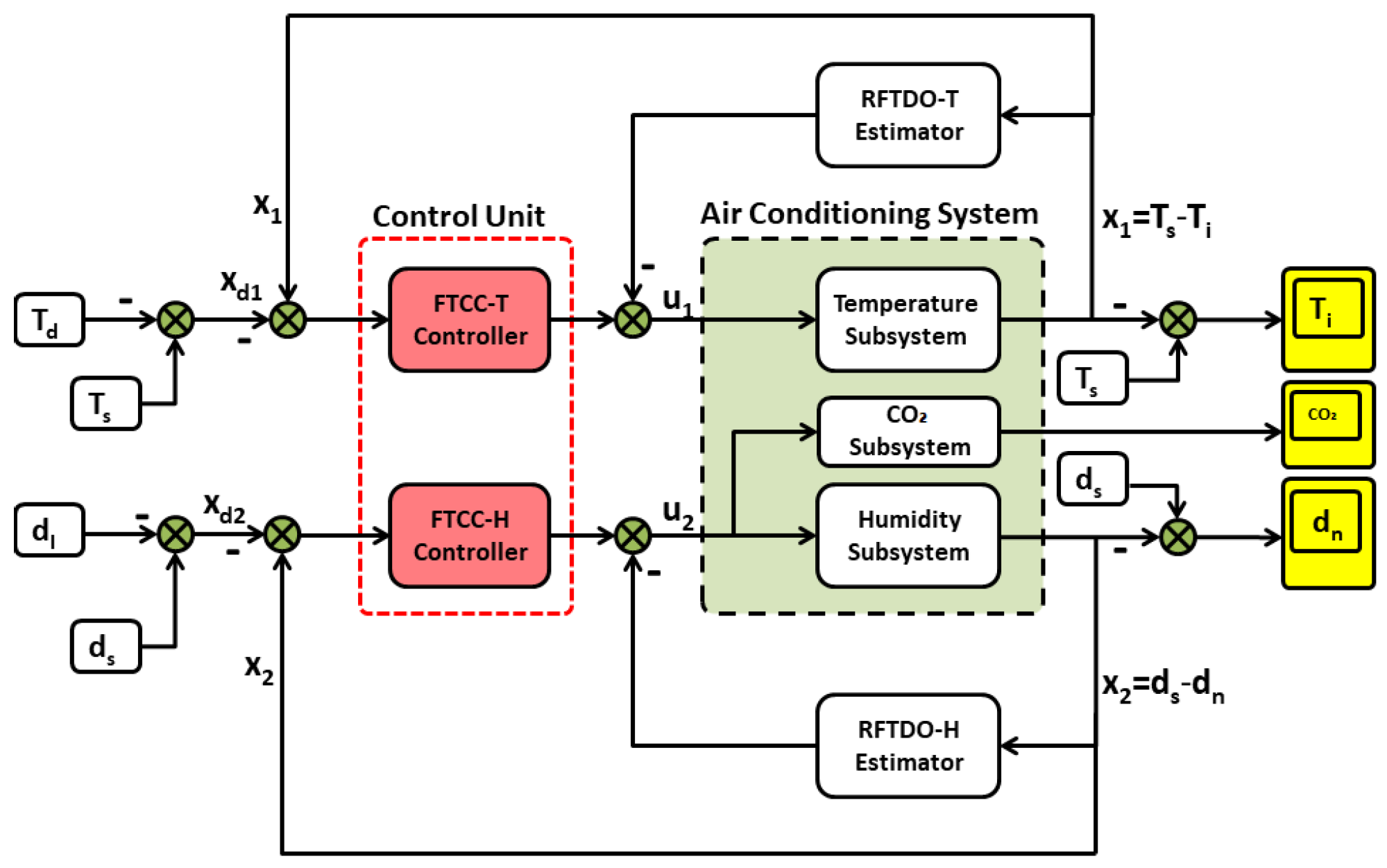This section gives the design of $u_1$ in (3) and $u_2$ in (4) for the temperature and humidity control, respectively, of the air conditioning system using the output feedback finite time composite control (FTCC) based on a novel robust finite time disturbance observer (RFTDO). For concise representation in this paper, the design procedure of $u_1$ for the temperature regulation is presented. Similarly, the other control input $u_2$ can be built for the humidity regulation. Thus, the RFTDO-T-based FTCC-T and the RFTDO-H-based FTCC-H are designed the control laws $u_1$ and $u_2$ of the temperature and humidity subsystems, respectively, as shown in the block diagram in Figure 2, where CO₂ is estimated based on the humidity control.

4.1. Design of a RFTDO-T-Based FTCC-T Scheme for the Temperature Subsystem

In the following, we start with the design steps of the temperature control law $u_1$.

4.1.1. Design of the RFTDO-T Estimator

To design our new disturbance observer of RFTDO-T in this subsection, we first present the following assumption:

Assumption 1. 

The lumped disturbances $D_1\left(x_1,d_1,t\right)$ and $D_2\left(x_2,d_2,t\right)$ of the temperature and humidity subsystem, respectively, existed in the system dynamics Equation (7) are differentiable with respect to time and there exist positive constants $D_{1max}$ and $D_{2max}$ such that their derivatives are bounded, satisfying |${\dot{D}}_i\left(t\right)$| ≤ $D_{imax}$ for $i$ = 1, 2.

Now, to estimate $D_1$, recall the temperature subsystem dynamics from Equation (7) as follows:

$${\dot{x}}_1=D_1\left(x_1,d_1,t\right)+b_{10}{u}_1\left(t\right)$$

(9)

where $D_1$ represents the lumped disturbance associated with the temperature dynamics, for which the derivative with respect to time is bounded as clarified in Assumption 1.

Let us consider the $x_{12}\left(t\right)=D_1\left(x_1,d_1,t\right)$ as an extended state and ${\dot{D}}_1\left(x_1,d_1,t\right)=h_1\left(t\right).$ Then, the dynamic of the air conditioning system Equation (9) can be rewritten:

$$\{ \begin{array}{c}{\dot{x}}_1\left(t\right)=x_{12}\left(t\right)+b_{10}{u}_1\left(t\right)\\ \\ {\dot{x}}_{12}\left(t\right)=h_1\left(t\right).\end{array}$$

(10)

To estimate the lumped disturbance $D_1\left(x_1,d_1,t\right)$ in the temperature dynamics Equation (7), the RFTDO-T is designed for the extended temperature subsystem dynamics Equation (10) as

$${\widehat{\dot{x}}}_1\left(t\right)={\widehat{x}}_{12}+b_{10}{u}_1\left(t\right)+l_{11}{\tilde{e}}_1\left(t\right){ }^{{\gamma }_{o1}}$$

$${\widehat{\dot{x}}}_{12}\left(t\right)=l_{12}{\tilde{e}}_1\left(t\right){ }^{(2{\gamma }_{o1}-1)}+{\phi }_1\left({\omega }_1\Delta {\tilde{e}}_1 \left(t\right)\right)$$

(11)

where ${\tilde{e}}_1\left(t\right)=x_1\left(t\right)-{\widehat{x}}_1\left(t\right)$ is the estimation error, ${\widehat{x}}_1\left(t\right)$, ${\widehat{x}}_{12}\left(t\right)$ are the estimations of states $x_1\left(t\right)$ and $x_{12}\left(t\right)$, respectively, $l_{11}$, $l_{12}$ and ${\omega }_1$ are the positive adjustable gains of RFTDO estimator, and ${\gamma }_{01}$ is the observer exponent. According to the observer design Equation (11), ${\widehat{x}}_{12}\left(t\right)$ is the estimation of $D_1\left(x_1,d_1,t\right)$. Moreover, the nonlinear function ${\phi }_1\left({\chi }_1\right)$ satisfies:

$${\phi }_1\left({\chi }_1\right)=\{ \begin{array}{c}-1, {\chi }_1\le -{\frac{\pi }{2}}_{ }\\ \sin \left({\chi }_1\right), -\frac{\pi }{2}\le {\chi }_1\le \frac{\pi }{2} .\\ \\ 1, {\chi }_1\le {\frac{\pi }{2}}_{ }\end{array}$$

(11a)

According to the bandwidth parameterization concept [47], the RFTDO-T gains in (11) can be calculated properly as follows:

$$l_{11}=2L_1 and l_{12}={\left(L_1\right)}^2$$

(11b)

where $L_1$ is the observer bandwidth of the RFTDO-T (11).

Theorem 1. 

In regard to Assumption 1, when the observer gains of the temperature dynamics Equation (9) are properly tuned, the estimation error of the RFTDO-T estimator Equation (11) converges to zero in finite time instance. Thus, we prove this Theorem in Appendix A.

4.1.2. Design of FTCC-T for the Temperature Subsystem

In this subsection, the FTCC-T including disturbance rejection term ${\widehat{x}}_{12}\left(t\right)$is designed for temperature dynamics Equation (9) as follows:

$$u_1\left(t\right)=\frac{1}{b_{10}}\left[k_1\lfloor e_1\left(t\right)\rceil { }^{{\alpha }_1}-{\widehat{x}}_{12}\left(t\right)\right]$$

(12)

with

$$e_1\left(t\right)=T_d\left(t\right)-T_i\left(t\right)$$

where $k_1>0$ is the control gain to be tuned, $0<{\alpha }_1<1$ is the control fractional power, $e_1\left(t\right)$ is the tracking error of temperature, $T_d\left(t\right)$ is the reference temperature command, and ${\widehat{x}}_{12}\left(t\right)$ is the estimated lumped disturbance by the finite time observer designed in (11).

Theorem 2. 

Regarding that the temperature dynamics Equation (9) is subject to the lumped disturbance satisfying Assumption 1. For a given feedback control gain $k_1>0,$ the output error of temperature, $e_1\left(t\right),$ is bounded and converges to zero in a finite-time. This theorem is proved in Appendix B.

4.2. Design of RFTDO-H-Based FTCC-H Scheme for Humidity Subsystem

In the following, we start with the design steps of the humidity control law.

4.2.1. Design of the RFTDO-H for the Humidity Subsystem

In this subsection, our new RFTDO is designed for the humidity dynamics. To estimate$D_2$, recall the humidity subsystem dynamics from (7) as follows:

$${\dot{x}}_2\left(t\right)=D_2\left(x_2, d_2,t\right)+b_{20}{u}_2\left(t\right)$$

(13)

where $D_2$ represents the lumped disturbance associated with the humidity dynamics, for which the disturbance derivative with respect to time is bounded as clarified in Assumption 1.

Similarly, let us consider the $x_{22}\left(t\right)=D_2\left(x_2,d_2,t\right)$ as an extended state and ${\dot{D}}_2\left(x_2,d_2,t\right)=h_2\left(t\right)$. Then, the humidity dynamic of the air conditioning system (13) can be rewritten as follows:

$$\{\begin{array}{c}{\dot{x}}_2\left(t\right)=x_{22}\left(t\right)+b_{20}{u}_2\left(t\right)\\ {\dot{x}}_{22}\left(t\right)=h_2\left(t\right).\end{array}$$

(14)

To estimate the lumped disturbance ${\widehat{D}}_2\left(x_2,d_2,t\right)$ in the humidity dynamics (7), the RFTDO-H is designed for the extended humidity subsystem dynamics (14) as

$${\widehat{\dot{x}}}_2\left(t\right)={\widehat{x}}_{22}\left(t\right)+b_{20}{u}_2\left(t\right)+l_{21}\lfloor {\tilde{e}}_2\left(t\right)\rceil { }^{{\gamma }_{o2}}$$

$${\widehat{\dot{x}}}_{22}\left(t\right)=l_{22}\lfloor {\tilde{e}}_2\left(t\right)\rceil { }^{(2{\gamma }_{o2}-1)}+{\phi }_2\left({\omega }_2\Delta {\tilde{e}}_2\left(t\right)\right)$$

(15)

where ${\tilde{e}}_2\left(t\right)=x_2\left(t\right)-{\widehat{x}}_2\left(t\right)$ is the estimation error; ${\widehat{x}}_2\left(t\right)$ and ${\widehat{x}}_{22}\left(t\right)$ are the estimations of states $x_2\left(t\right)$ and $x_{22}\left(t\right)$, respectively; $l_{21}$, $l_{22}$, and ${\omega }_2$ are the positive adjustable gains of the RFTDO-H estimator; and ${\gamma }_{o2}$ is the observer exponent. According to the observer design (14), ${\widehat{x}}_{22}\left(t\right)$ is the estimation of $D_2\left(x_2,d_2,t\right)$. Moreover, the nonlinear function ${\phi }_2\left({\chi }_2\right)$ satisfies

$${\phi }_2\left({\chi }_2\right)=\{\begin{array}{c}-1, {\chi }_2\le -\frac{\pi }{2} \\ \sin \left({\chi }_2\right), -\frac{\pi }{2}\le {\chi }_2\le \frac{\pi }{2} .\\ 1, {\chi }_2\ge \frac{\pi }{2} \end{array}$$

(15a)

According to the bandwidth parameterization concept [47], the RFTDO-H gains (15) can be calculated properly as follows:

$$l_{21}=2L_2 and l_{22}={\left(L_2\right)}^2$$

(15b)

where $L_2$ is the observer bandwidth of the RFTDO-H (15).

Theorem 3. 

Based on Assumption 1, when the observer gains of the humidity dynamics Equation (33) are properly chosen, the estimation error of the RFTDO-H estimator (15) converges to the zero in finite time instance.

Proof of Theorem 3. 

To avoid duplication, the stability proof is on a similar line of Proof of Theorem 1 given in Appendix A. Thus, we omit the stability proof of the RFTDO-H estimator (15). □

4.2.2. Design of the Finite-Time Composite Humidity Controller

In this subsection, finite time composite control humidity (FTCC-H) including disturbance rejection term ${\widehat{x}}_{22}\left(t\right)$ is designed for the humidity dynamics (13) as follows:

$$u_2\left(t\right)=\frac{1}{b_{20}}\left[k_2\lfloor e_2\left(t\right)\rceil { }^{{\alpha }_2}-{\widehat{x}}_{22}\left(t\right)\right]$$

(16)

with

$$e_2\left(t\right)=d_l\left(t\right)-d_n\left(t\right)$$

where $k_2>0$ is the control gain to be tuned, $0<{\alpha }_2<1$ is the control fractional power, $e_2\left(t\right)$ is the tracking error of humidity, $d_l(t$) is the reference humidity command, and ${\widehat{x}}_{22}\left(t\right)$ is the estimated lumped disturbance by the RFTDO-H designed in (15).

Theorem 4. 

Regarding that the humidity model (4) is subject to the lumped disturbance satisfying Assumption 1. For a given feedback control gain $k_2>0$, the output error of humidity $e_2\left(t\right)$ is bounded and converges to zero in a finite-time. This theorem is proved in Appendix C.

4.3. Stability Analysis of the Whole Closed Loop System

The analysis of the finite time stability of the whole closed loop system that consists of the error dynamics Equations (A15) and (A21) has two steps. First, we prove that $e_1\left(t\right)$ and $e_2\left(t\right)$ are bounded when $t\in \left(0,T_f\right]$, where $T_f=\max \left(t_{f1},t_{f2}\right)$ is the time constant. Second, the whole closed loop stability is finite time at $t>T_f$.

Step 1: when $t\in \left(0,T_f\right]$, the Lyapunov candidate function along the closed loop system dynamics Equations (A15) and (A21) is considered as

$$V=\frac{1}{2}{e}_1^2+\frac{1}{2}{e}_2^2=V_{c1}+V_{c2}$$

(17)

Subsequently, the qualities of the closed loop stability of the temperature and the humidity dynamics in Equations (A15) and (A21), respectively, are combined based on the total Lyapunov as

$$V=V_{c1}+V_{c2}=-2k_1{V}_{c1}-2k_2{V}_{c2}+\frac{1}{2}{\left|{\tilde{e}}_{12max}\right|}^2+\frac{1}{2}{\left|{\tilde{e}}_{22max}\right|}^2$$

(18)

From (A19) and (A23), we can conclude that the boundedness of $e_1\left(t\right)$ and $e_2\left(t\right)$ is guaranteed.

Step 2: when $t>T_f$, the closed loop dynamics of the controlled temperature and humidity dynamics is recalled and reduced to

$${\dot{e}}_1\left(t\right)=-k_1\lfloor e_1\left(t\right)\rceil { }^{{\alpha }_1}$$

$${\dot{e}}_2\left(t\right)=-k_2\lfloor e_2\left(t\right)\rceil { }^{{\alpha }_2}$$

(19)

Choosing the same Lyapunov function as in Equation (17), when $t>T_f$, the differentiation of $V$ is

$$\begin{array}{c}\dot{V}=e_1{\dot{e}}_1+e_2{\dot{e}}_2\\ =k_1{\left|e_1\right|}^{{\alpha }_1+1}+k_2{\left|e_2\right|}^{{\alpha }_2+1}\\ =-2^{\frac{{\alpha }_1+1}{2}}{k}_1{\left(\frac{1}{2}{e}_1\right)}^{\frac{{\alpha }_1+1}{2}}-2^{\frac{{\alpha }_2+1}{2}}{k}_2{\left(\frac{1}{2}{e}_2\right)}^{\frac{{\alpha }_2+1}{2}}\end{array}$$

(20)

Using (A19) and (A23), we have

$$\begin{array}{c}\dot{V}\le -2^{\frac{{\alpha }_1+1}{2}}{k}_1{\left(\frac{1}{2}{e}_1\right)}^{\frac{{\alpha }_1+1}{2}}-2^{\frac{{\alpha }_2+1}{2}}{k}_2{\left(\frac{1}{2}{e}_2\right)}^{\frac{{\alpha }_2+1}{2}}\\ =-2^{\frac{{\alpha }_1+1}{2}}{k}_1{\left(V_{c1}\right)}^{\frac{{\alpha }_1+1}{2}}-2^{\frac{{\alpha }_2+1}{2}}{k}_2{\left(V_{c2}\right)}^{\frac{{\alpha }_2+1}{2}}\le 0\end{array}$$

(21)

Hence, at $t>T_f$

$$\dot{V}+2^{\frac{{\alpha }_1+1}{2}}{k}_1{\left(V_{c1}\right)}^{\frac{{\alpha }_1+1}{2}}+2^{\frac{{\alpha }_2+1}{2}}{k}_2{\left(V_{c2}\right)}^{\frac{{\alpha }_2+1}{2}}\le 0.$$

(22)

Therefore, the tracking errors $e_1$ and $e_2$ approach zero in finite time, i.e., the temperature and humidity can track the reference values $T_d$ and $d_l$ in finite time.

4.4. Estimation of Indoor CO₂ Concentration

To guarantee that the estimated air concentration in the office space will stay fresh, full fresh air input is used by the latent heat control system. The amount of the indoor CO₂ concentration estimation model is given by:

$$\dot{C}=\frac{C_{out}}{V}{V}_v\left(t\right)+Q_p+18n-\frac{C}{V}\left(V_v\left(t\right)-L\right)$$

(23)

with

$$V_v\left(t\right)=\frac{u_2\left(t\right)}{d_s-d_n}$$

where $C$ is the indoor CO₂ concentration, $Q_p$ is the pollutant emission rate, n is the number of people in the office building, and $V_v\left(t\right)$ is the mechanical ventilation (m³/h) of the office. In (23), the control law $u_2\left(t\right)$ has been designed in the FTCC-H (16).

For better understanding the philosophy of the proposed control algorithm, the flowchart of the proposed control is shown in Appendix D (Figure A1). For reproducibility of the paper idea, the Simulink Code of the proposed method is given in Appendix E (Figure A2).

Remark 1. 

When${\alpha }_1={\alpha }_2={\gamma }_{o1}={\gamma }_{o2}=1$, the control law of FTCC-T (11), (12) will reduce to the linear composite control (called counterpart controller), which is given as

$$u_1\left(t\right)=\frac{1}{b_{10}}\left[k_1{e}_1\left(t\right)-{\widehat{x}}_{12}\left(t\right)\right]$$

(24)

and

$${\dot{\widehat{x}}}_1\left(t\right)={\widehat{x}}_{12}\left(t\right)+b_{10}{u}_1\left(t\right)+l_{11}{\tilde{e}}_1\left(t\right)$$

$${\dot{\widehat{x}}}_{12}\left(t\right)=l_{12}{\tilde{e}}_1\left(t\right)+{\phi }_1\left({\omega }_1\Delta {\tilde{e}}_1\left(t\right)\right)$$

(25)

Similarly, the control law of FTCC-H (15), (16) will reduce to the linear composite control (called counterpart controller) as follows

$$u_2\left(t\right)=\frac{1}{b_{20}}\left[k_2{e}_2\left(t\right)-{\widehat{x}}_{22}\left(t\right)\right]$$

(26)

and

$${\dot{\widehat{x}}}_2\left(t\right)={\widehat{x}}_{22}\left(t\right)+b_{20}{u}_2\left(t\right)+l_{21}{\tilde{e}}_2\left(t\right)$$

$${\dot{\widehat{x}}}_{22}\left(t\right)=l_{22}{\tilde{e}}_1\left(t\right)+{\phi }_2\left({\omega }_2\Delta {\tilde{e}}_2\left(t\right)\right)$$

(27)

In this case, the tracking error trajectories will asymptotically converge to zero instead of finite-time convergence. That is, robust finite-time composite control will illustrate a faster convergence rate than the linear counterpart control, which will be shown by comparing the responses curves of the simulation section of this paper.

Remark 2. 

By setting${\phi }_1\left({\omega }_1\Delta {\tilde{e}}_1\left(t\right)\right)={\phi }_2\left({\omega }_2\Delta {\tilde{e}}_2\left(t\right)\right)=0$, the FTCC-T control law (11), (12) will reduce to the well-known active disturbance rejection control (ADRC) for the temperature subsystem, which is given as

$$u_1\left(t\right)=\frac{1}{b_{10}}\left[k_1\lfloor e_1\left(t\right)\rceil { }^{ }-{\widehat{x}}_{12}\left(t\right)\right]$$

(28)

and

$${\dot{\widehat{x}}}_1\left(t\right)={\widehat{x}}_{12}\left(t\right)+b_{10}{u}_1\left(t\right)+l_{11}{\tilde{e}}_1\left(t\right)$$

$${\dot{\widehat{x}}}_{12}\left(t\right)=l_{12}{\tilde{e}}_1\left(t\right)$$

(29)

Similarly, the FTCC-H (15), (16) will reduce to the ADRC for the humidity subsystem follows:

$$u_2\left(t\right)=\frac{1}{b_{20}}\left[k_2\lfloor e_2\left(t\right)\rceil { }^{ }-{\widehat{x}}_{22}\left(t\right)\right]$$

(30)

and

$${\dot{\widehat{x}}}_2\left(t\right)={\widehat{x}}_{22}\left(t\right)+b_{20}{u}_2\left(t\right)+l_{21} {\tilde{e}}_2\left(t\right)$$

$${\dot{\widehat{x}}}_{12}\left(t\right)=l_{12}{\tilde{e}}_1\left(t\right)$$

(31)

In this case, the tracking errors$e_1\left(t\right)$and$e_2\left(t\right)$trajectories will asymptotically converge to zero instead of finite-time convergence. That is, the robust FTCC-T and FTCC-H control laws will illustrate not only a faster convergence rate, but also a higher robustness than the ADRC, which is shown by comparing the curves responses of the simulation section.

Remark 3. 

It is worth noting that our novel estimators in (11) and (15) are designed based on three parameters, including observer bandwidth $L_i$, exponent ${\gamma }_{oi}$, robustness gain ${\omega }_i,$ for $i$ = 1, 2. Therefore, we summarize and discuss the tuning process of the parameters of the proposed control scheme and give a suggested guideline on how to design those estimators. The tuning process of the proposed observers includes three key selections of the parameters as follows:

(1)

Selection of$L_i$: Large observer bandwidth$L_i$increases the estimation accuracy, but overlarge observer bandwidth L_i cause negative effects such as a peaking phenomenon. Thus, based on the selection of L_i, we have to have an optimal tradeoff between the estimation accuracy and peaking phenomenon.

(2)

Selection of ${\gamma }_{oi}$: Large observer fractional powers ${\gamma }_{oi}$ lead to not only fast convergence of the estimation error to zero in a shorter finite time, but also increasing disturbance rejection ability. However, overlarge fractional powers cause the chattering behaviors in both estimations and control inputs $u_1$ and $u_2$. Generally, the fractional exponents in (11) and (15) have values between 0 and 1. If the values are close to 0, the convergence speed of estimations is fast, but the estimations and control inputs are highly affected by the chattering, whereas if the values are near 1, the chattering can be suppressed, but the estimations convergence is slow. Therefore, it is required to have an optimal balance between estimation convergence rate and chattering.

(3)

Selection of ω_i: A suitable large gain ω_i can lead a strong robustness performance of the estimators (11) and (15). Moreover, the estimation errors convergences to zero are speeded up remarkably.

Remark 4. 

For more details about how to design the presented estimator in (11), the finite time disturbance observer (estimator) of the temperature loop denoted by the RFTDO-T is designed based on the availability of the temperature state x₁ and u₁ as expressed in (11). Generally, the structure of the RFRDO has correction terms which represented in the term with the fractional power γ_o1 existed in the first and second channel of the estimator structure. Our estimator objective is to minimize the correction terms as much as possible by increasing the estimator bandwidth in (11b); thus, the image of this estimator can be close the original system dynamics. Accordingly, the disturbance estimation in the loop temperature is the output of the RFTDO-T, which can track its true value accurately at the finite time. To this end, to the best of authors’ knowledge, the nonlinear function term ϕ in the second channel of the estimator is newly used in the RFTDO-T as the robustness term against the first derivative of the disturbance h₁ in the dynamics (10). Based on correction and robustness terms, we will have accurate disturbance estimation that can be incorporated and compensated in the control law in (12). To avoid repetition, the explanation above can be used for the RFTDO-H (15) in the humidity loop.

5. Simulation Results

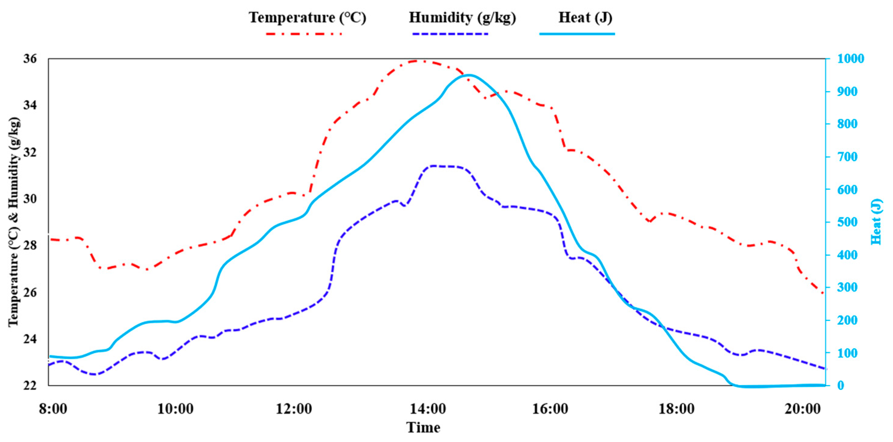
To carry out the simulation model of the air conditioning system, MATLAB/Simulink is used. In this section, the effectiveness of the proposed output feedback is evaluated through the numerical simulations of an air conditioning system. The solver of simulations is set as fixed-step and its size is chosen as 0.1 ms. The numerical values of the air conditioning system parameters used in the mathematical model are selected to be same as that in [9] and are listed in Table 1. Based on the data taken from the article in [9], the heat produced by the sunlight radiation through the glass windows (in Joules per square meter per second), the outdoor temperature, and the outdoor humidity change are plotted in Figure 3.

For comparison purposes, three different control strategies are also applied for the air conditioning system: the linear counterpart controller; the active disturbance rejection controller, and the sliding mode controller are labelled counterpart, ADRC, and SMC in the simulation curves, respectively. Based on Remark 1 in this work, the first scheme of comparison is the linear composite counterpart controller, which was given in (24) and (26). Based on Remark 2, the second scheme of comparison is the ADRC, which has been given in (28) and (30).

Moreover, the third method of comparison is the output-based SMC for the temperature and humidity subsystems system (5), respectively, are designed [9] as:

$$u_i\left(t\right)=-\frac{1}{b_{i0}}\left[f_{i0}\left(x_i,t\right)+c_i{e}_i\left(t\right)-{\dot{x}}_{di}+K_i{s}_i+k_i\sin \left(s_i\right)\right]\mathrm{for} i=1,2.$$

(32)

with

$$s_i\left(t\right)=e_i\left(t\right)+c_i{\displaystyle \int }{e}_i\left(t\right)dt \mathrm{for} i=1,2.$$

(33)

where $c_i$, $K_i$, and $k_i$ for $i=1,2$ are positive constants.

Remark 5. 

The reason for choosing these comparative control algorithms, including counterpart, ADRC, and SMC is that the structure of these algorithms is similar owing to the use of disturbance observer-based controller techniques. According to Remarks 1 and 2, the comparative counterpart and ADRC schemes are derived from the proposed control scheme as in (24)–(27) and (28)–(31), respectively, by taking the special case of control parameters into account. For the sake of variety and distinct from the observer-based controller technique, we also apply the SMC (32) approach which is one of the robust control strategies and does not need an accurate system modelling. For another comparison purpose, the SMC in (32) can be reduced from the proposed method without incorporating the RFTDO-T and RFTDO-H estimators. Consequently, we possess unified specifications of the comparative controls’ parameters that can be selected equally to ensure the fairness of comparison in terms of control and parameters’ selection, referring to Remarks 1 and 2, and

Table 2. Control parameters.

Controller	Parameters
Proposed	$k_1=5, {\alpha }_1=0.4, {\gamma }_{o1}=0.85, L_1=30, {\omega }_1=5000$  $k_2=2.3, {\alpha }_2=0.8, {\gamma }_{o2}=0.8, L_2=23, {\omega }_2=10,000$
Counterpart	$k_1=5, {\alpha }_1=1, {\gamma }_{o1}=1, L_1=30, {\omega }_1=5000$  $k_2=2.3, {\alpha }_2=1, {\gamma }_{o2}=1, L_2=23, {\omega }_2=10,000$
ADRC	$k_1=5, {\alpha }_1=1, {\gamma }_{o1}=1, L_1=30, {\omega }_1=0$  $k_2=2.3, {\alpha }_2=1, {\gamma }_{o2}=1, L_2=23, {\omega }_2=0$
SMC	$c_1=5, K_1=2.5, k_1=0.6$  $c_2=2.3, K_2=7, k_1=0.6$

, respectively. In brief, the control bandwidth is a common specification among proposed and comparative controllers, which is, of course, chosen equally.

Two groups of simulated results are conducted to verify this work. The first mission is the temperature and humidity regulation under the nominal case and the second would be this regulation under external disturbances. These missions are chosen to actively analyze the effect of the proposed controller on the variables of temperature, humidity, and CO₂ of the air conditioning system. The proposed and comparative controllers’ parameters are selected as in Table 2. Accordingly, with reference to Remark 3, such parameters are treated equally in order to ensure the fairness of comparison taking into account that most of the parameters are common in the schemes.

(1)

Regulation Task under the nominal system case: In this task, the temperature and humidity in the air conditioning system are desired to follow trajectories represented by step references. The objective here is to find and compare the estimation error and tracking curves of the proposed method against the comparative controllers. To begin with this, the air conditioning system model is subject to the following input references $T_d$= 25 $°\mathrm{C}$ and $d_d$= 12 g/kg.

Figure 4 shows the estimation performance of the RFTDO-T for the nominal temperature and humidity subsystems’ dynamics. As demonstrated in Figure 4a,b, the estimation error ${\tilde{e}}_1$ of $x_1$ and the lumped disturbance estimation error ${\tilde{e}}_{12}$ of $x_{12}$ in the temperature dynamics approach zero in finite time by the proposed RFTDO estimator compared to the linear DO estimator in the counterpart control and the ESO in the ADRC technique. Figure 4c,d, illustrate that the estimation error ${\tilde{e}}_2$ of $x_2$ and the lumped disturbance estimation error ${\tilde{e}}_{21}$ of $x_{21}$ in the humidity dynamics both approach zero in finite time by the Proposed RFTDO estimator in comparison to the comparative estimators. Accordingly, the lumped disturbance $D_1$ and $D_2$ in both the temperature and humidity subsystems can be estimated with high accuracy.

The simulation comparison of indoor temperature, humidity, and CO₂ responses of the air conditioning system are shown in Figure 5. From the results, it can be seen that the proposed methodology has a better performance than the ADRC, and SMC in terms of overshoot elimination, short settling time, and high accuracy steady state. From the simulation results, the settling time of the temperature and humidity profile under the proposed control are inferred to be about at 08:15 and 08:40, which are shorter than the comparative controls. In other words, the convergence rate of the proposed temperature and humidity control system is faster than the SMC, ADRC, and Counterpart schemes.

In addition, by using the fresh air input, the CO₂ concentration of the indoor air within a day is well estimated, considering that the office CO₂ concentration is 0.045% of the air at 8:00. One can also observe from Figure 5c that the air conditioning system with the robust FTCC-T and FTCC-H scheme has a CO₂ level below the maximum level of CO₂ of 0.1%. Based on that, we can ensure the freshness of the indoor air whilst meeting thermal comfort requirements. Furthermore, it can be seen from Figure 6a,b that the proposed control effort shows a lower input air volume of $G_s$ and $G_o$ as compared to others. More importantly, this leads to improving the energy consumption reduction under the proposed temperature and humidity control.

(2)

Regulation Task under Multi-source disturbances: In this case, two sinusoidal waveform disturbances are combined as a multi-sources disturbance. The amplitude and angular frequency of the first sinusoidal disturbance are A₁ = 10 °C or 0.5 g/kg.hr and ${\overline{\mathsf{\omega }}}_1$= 7 rad/hr, respectively. The second sinusoidal disturbance has amplitude and frequency of A₂ = $2 °\mathrm{C}$ or 0.1 g/kg.hr and ${\overline{\mathsf{\omega }}}_2$ = 4 rad/hr, respectively. More specifically, the temperature dynamics in (3) are subject to a net dual disturbance defined by $d_1\left(t\right)=10 \sin \left({\overline{\mathsf{\omega }}}_1 \mathrm{t}\right)+2\sin \left({\overline{\mathsf{\omega }}}_2 \mathrm{t}\right)$ in °C, while a net dual disturbance of $d_2\left(t\right)=0.5 \sin \left({\overline{\mathsf{\omega }}}_1 \mathrm{t}\right)+0.1\sin \left({\overline{\mathsf{\omega }}}_2 \mathrm{t}\right)$ g/kg.hr affects the humidity dynamics in (4). Note that such disturbances, $d_1\left(t\right)$ and $d_2\left(t\right)$, are depicted in Figure 7a,c, respectively, which are labelled as actual disturbances acting on the temperature and humidity dynamics and are plotted by black dash-dotted lines. As in Task 1, the ideal reference inputs of the temperature and moisture are kept in the current case.

The estimation errors of temperature, the lumped disturbance $D_1$ in the temperature dynamics in (6), humidity, and the lumped disturbance $D_2$ in the humidity dynamics in (6) are shown in Figure 6 where it can be observed that the estimation errors of the proposed disturbance observers rapidly approach zero in the finite time. It is obvious that the proposed control scheme has higher precision of the estimations than the ADRC and Counterpart schemes. To further evaluate the observation performance of the proposed disturbance observers, the estimation and its error of the net dual disturbance $d_1\left(t\right)$ and $d_2\left(t\right)$ that act on the temperature and humidity subsystem, are shown in Figure 7. From these plots, it is easy to find that the proposed observers’ design has an obvious observation performance improvement for the air conditioner system.

Based on the accurate estimations by the designed observers, Figure 8a,b. demonstrate that the fast convergence of the indoor temperature and humidity to their reference inputs are achieved by the proposed independent control. It can be seen that the convergence time of the temperature and humidity under the proposed method is roughly 15 min of operating the air conditioner and has oscillation free at the steady state region. However, the SMC exhibits a huge overshoot in the transient region and has the effect of the control chattering in the steady state region. Additionally, the comparative ADRC and counterpart does not settle and oscillates around the reference commands. From Figure 8c, for the same CO₂ circumstance in Task 1, the level of CO₂ concentration in the indoor air within a day is well estimated by the proposed method and is below the maximum level of the CO₂ of 0.1%. Consequently, we can keep the freshness of air indoor and meet the human comfort requirements even in the presence of the influence of the external disturbance on the conditioner.

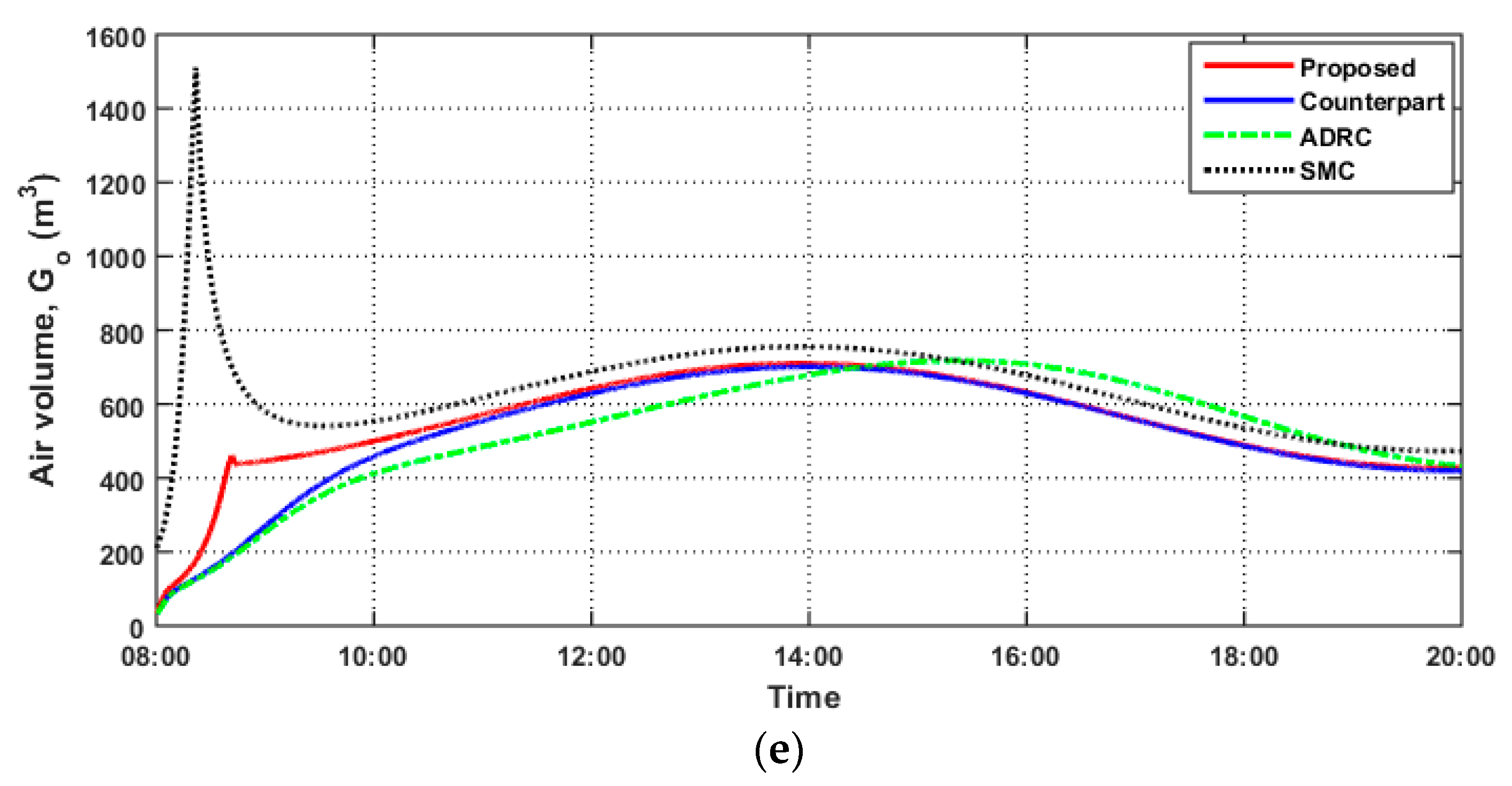
Furthermore, it can be seen from Figure 8d,e that the proposed control effort shows a lower the input air volume of $G_s$ and $G_o$ as compared to the other controllers. However, the SMC obviously suffers from the saturation and the chattering problem. Crucially, the proposed temperature and humidity controller improves energy consumption: there is a reduction in the energy required to run the system compared to the other controllers.

(3)

Regulation Task under HVAC system uncertainties (Task 3): In this task, we further investigate the robustness of the proposed scheme against the system uncertainties. Since the model of the considered system is an approximation of the real HVAC system, this model has some inaccuracies and uncertainties in some different parameters and unmodeled dynamics. To demonstrate this in the simulative case, system uncertainties can be introduced by varying with 20% of nominal values of n and L as listed in Table 1. This reflects an increase in the number of occupants from 10 to 12. In this case, the setpoint reference and external disturbances are kept as in Task 1 and 2, and other system parameters are kept unchanged.

Accordingly, the humidity dynamics are affected by these system uncertainties, in which the output variable of humidity regulation is shown in Figure 9. As demonstrated in Figure 9, the proposed observer-based control can quickly and precisely track the required setpoint from occupants because the proposed scheme has a strong performance with respect to system uncertainties rejection.

6. Conclusions

In this paper, an effective and robust FTCC method has been proposed for an air conditioning system. A new RFTDO technique based on output feedback, the FTCC has been proposed to minimize the influence of system uncertainties and disturbances on the system humidity and temperature outputs. The proposed control scheme not only guarantees humidity and temperature outputs converge to their reference points in finite time, but also maintains the robustness of control action. The finite time stability of the whole closed loop system has been guaranteed by using the Lyapunov theory. Extensive simulation results demonstrated that, overall, the effectiveness of the proposed controller outperforms both the conventional SMC and ADRC methods. Accordingly, the proposed controller offers better temperature, humidity, and CO₂ regulation accuracy. Furthermore, the proposed controller outcompetes the SMC and ADRC controllers in terms of reduced energy consumption, which is beneficial for businesses aiming to reduce ongoing energy costs and their carbon footprint. Future work will concentrate on applying the FTCC scheme based on RFTDO technique to different cities. In addition to that, future research will account for the time lag which is caused by distributed parameters in the system modelling that come from partial differential equations and can be approximated with a dead time or transport time. Moreover, the mathematical model of the HVAC system will be verified by focusing on and providing solutions for the differential equations used to establish that mathematical model. Furthermore, we will apply the proposed scheme on the real time HVAC system under the complex assumptions of non-step signals. To execute this future work, not only the C language, but also the Simulink blocks will be written in a step-by-step manner. This would be helpful for interested researchers to reproduce the experimental application of the proposed work.