


ANN-Based Method for Urban Canopy Temperature Prediction and Building Energy Simulation with Urban Heat Island Effect in Consideration


Abstract
1. Introduction
2. Approach
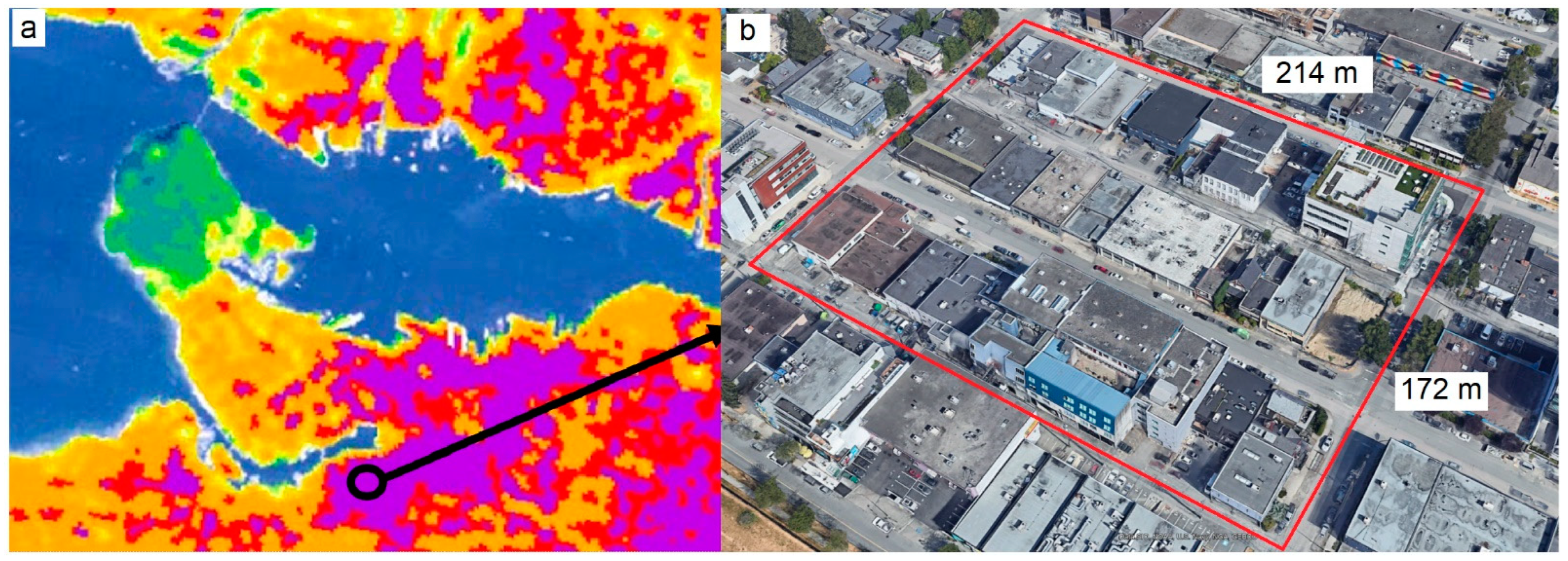
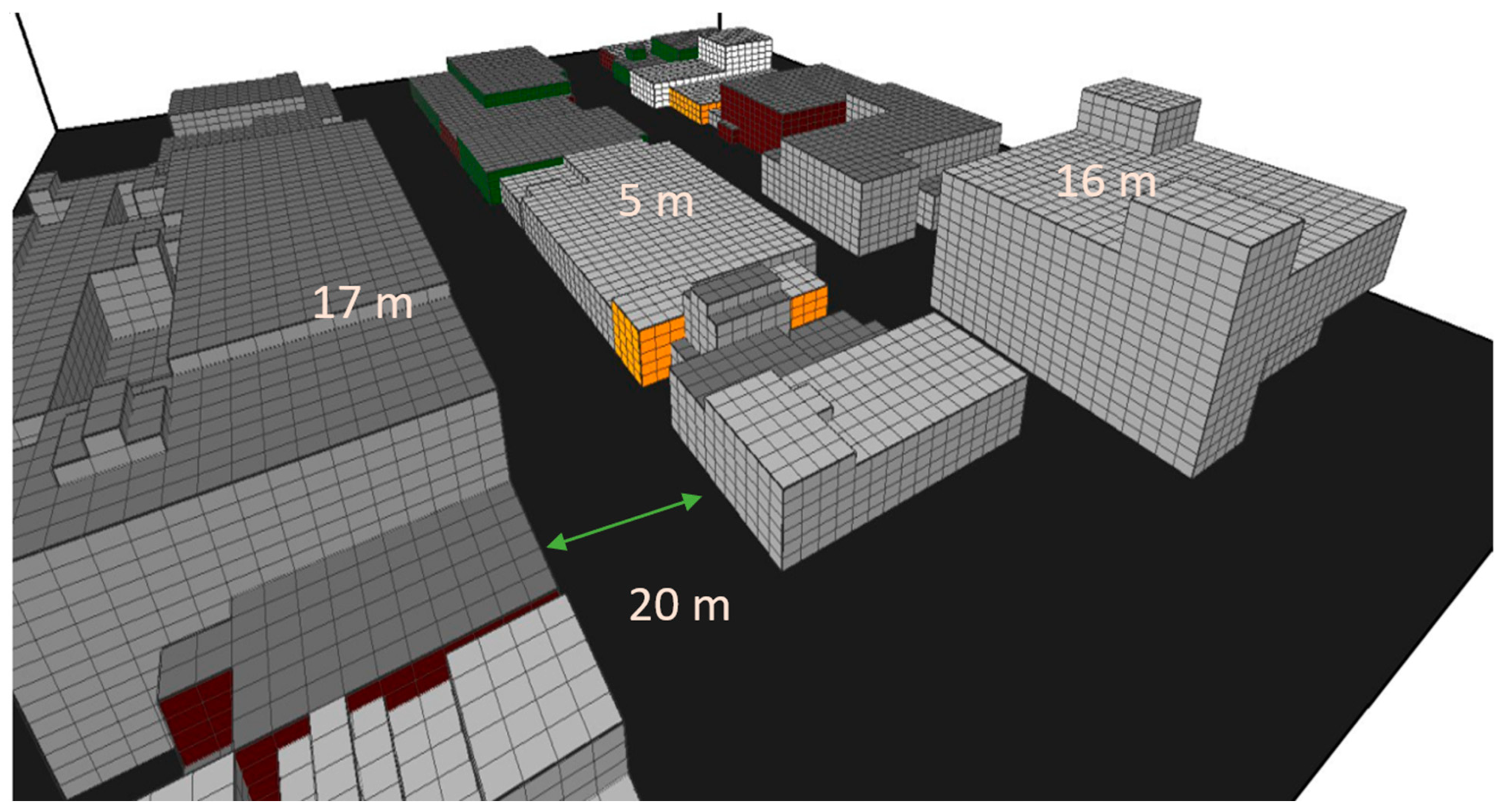
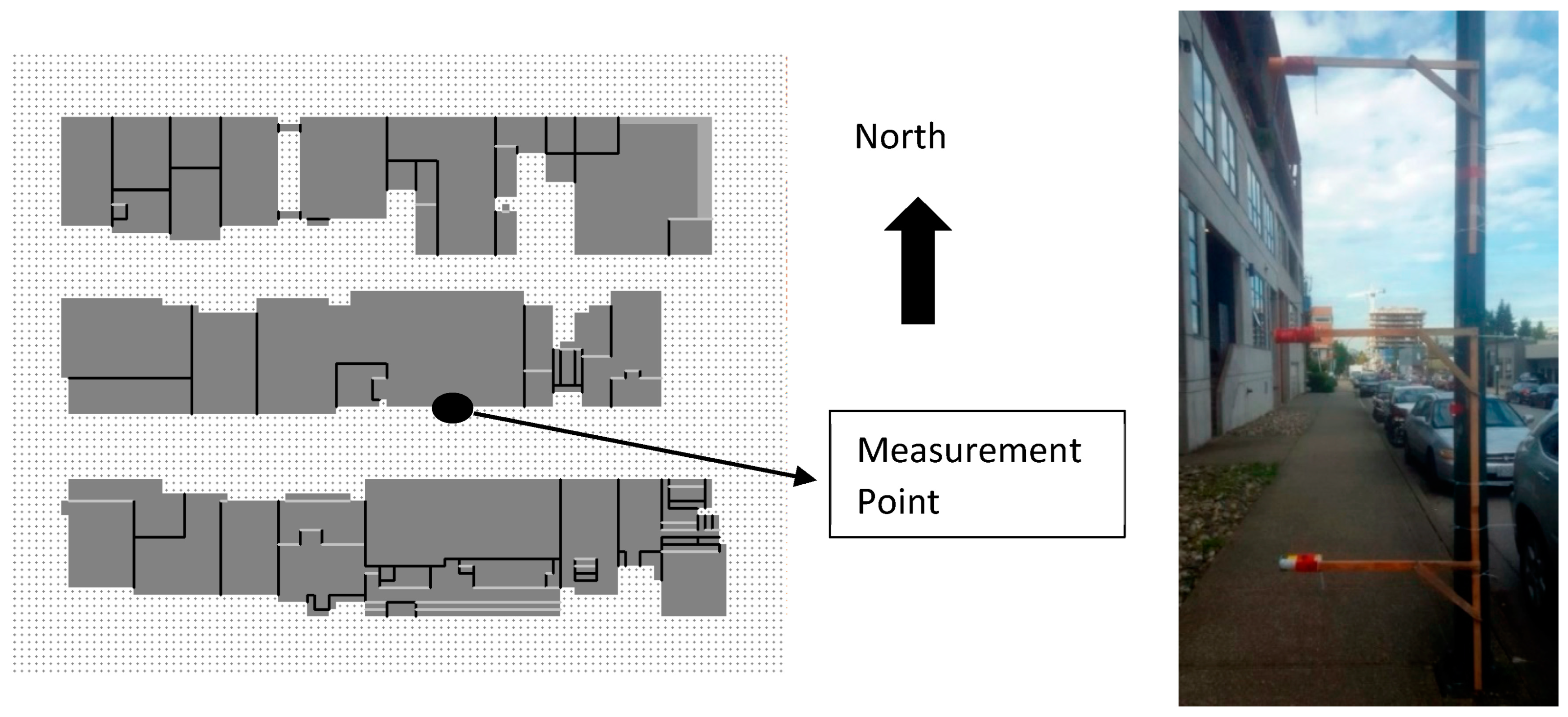
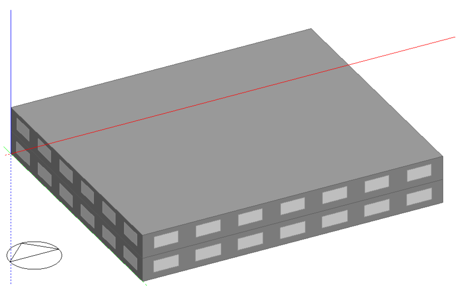
2.1. Study Area
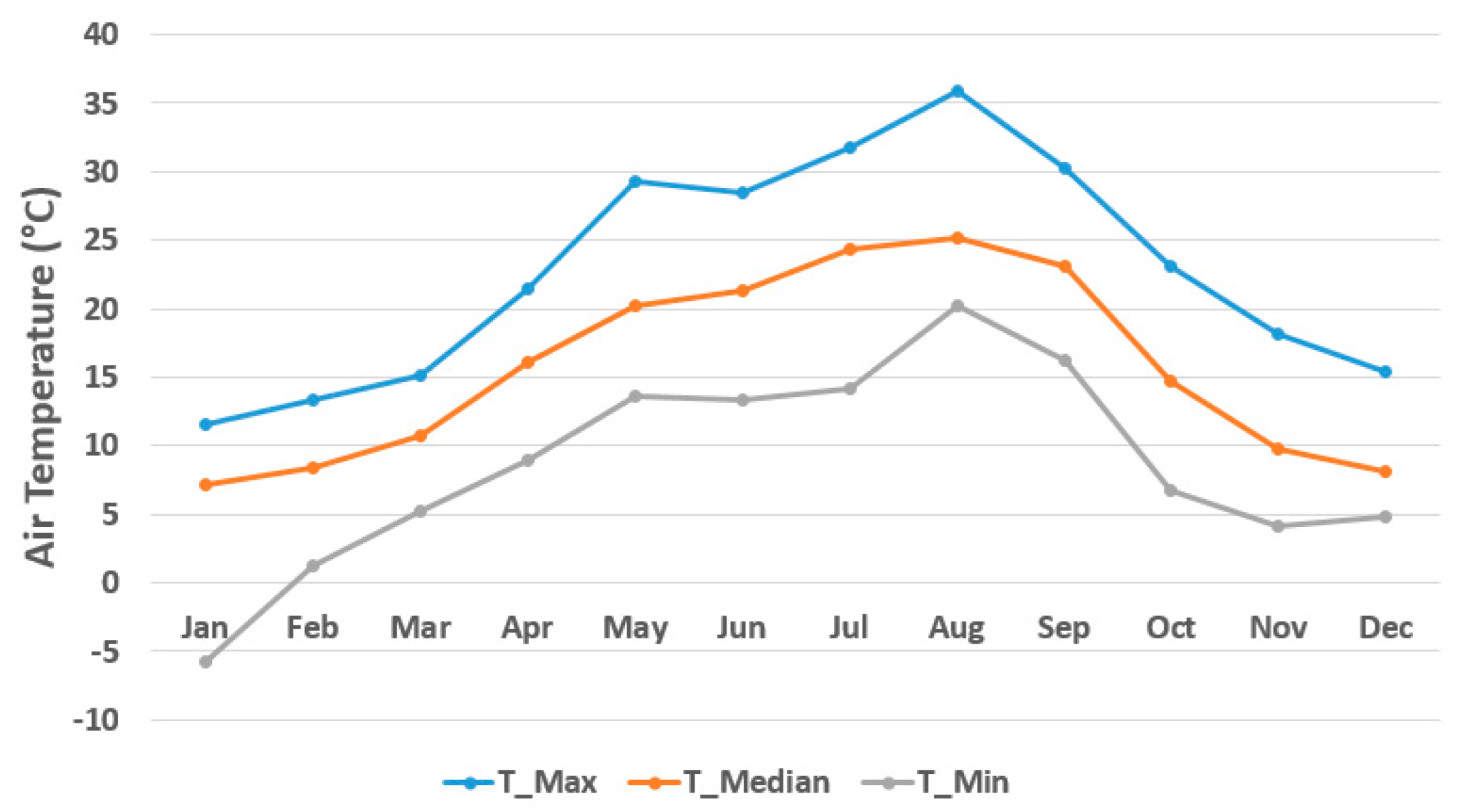
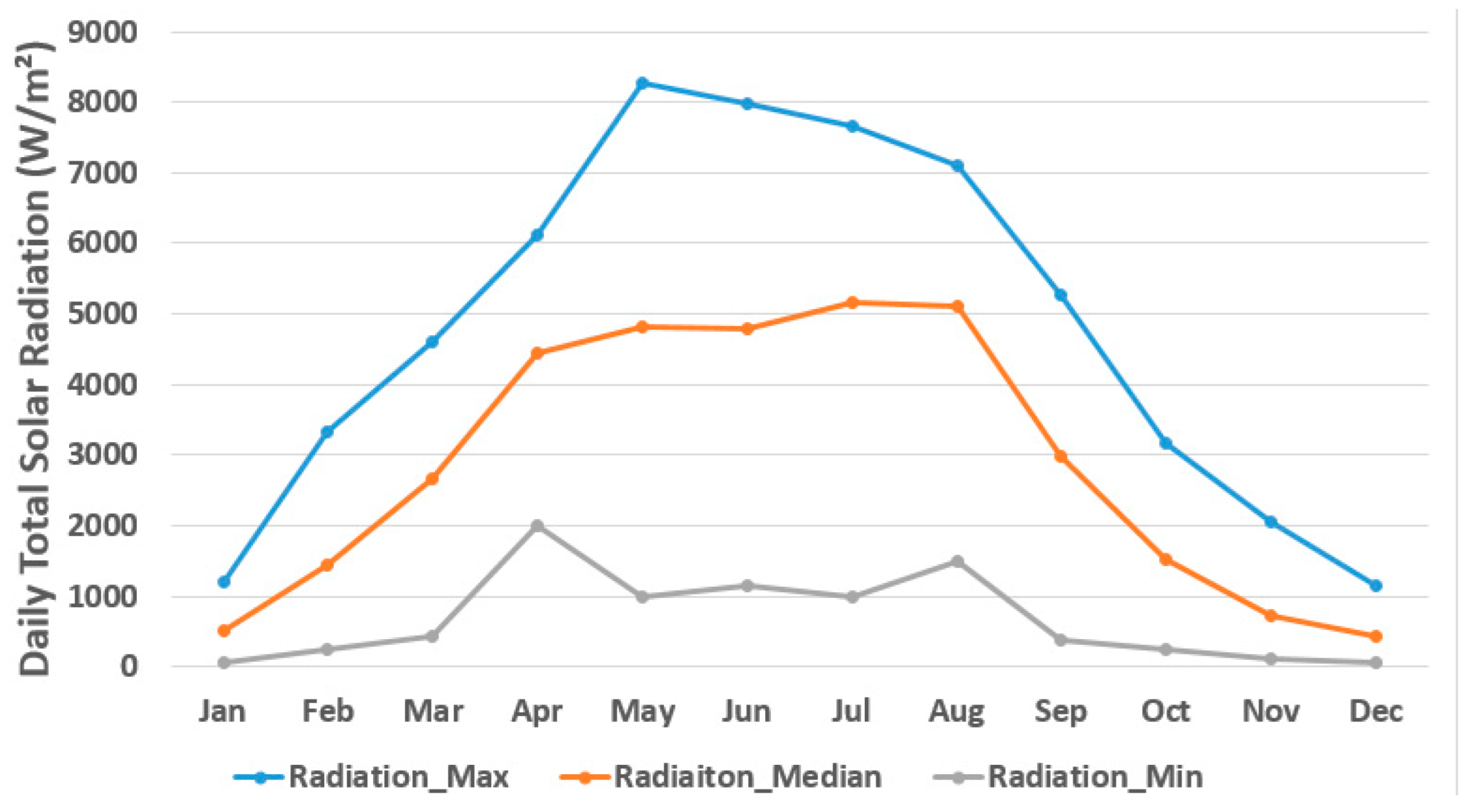
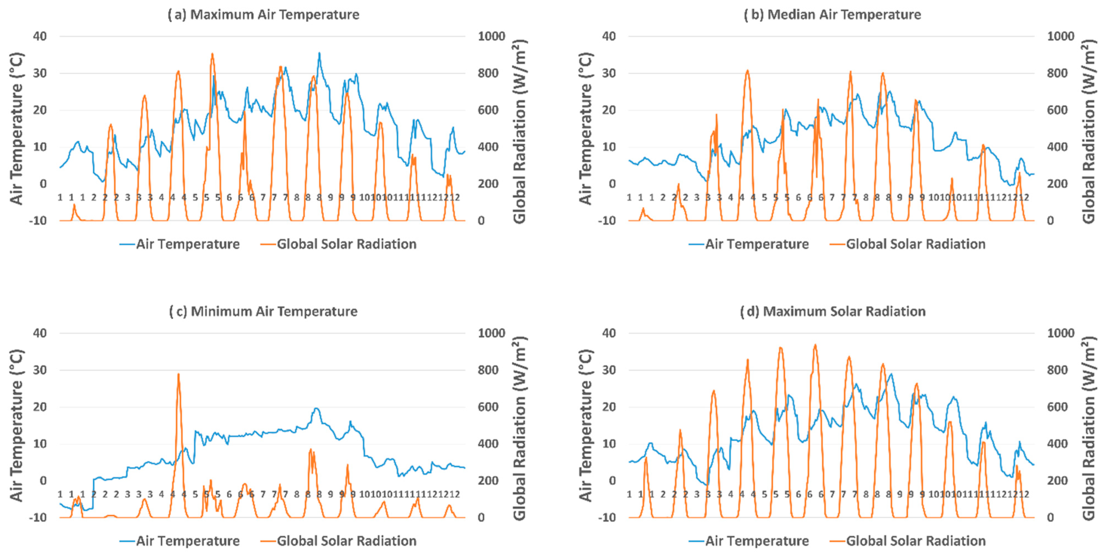
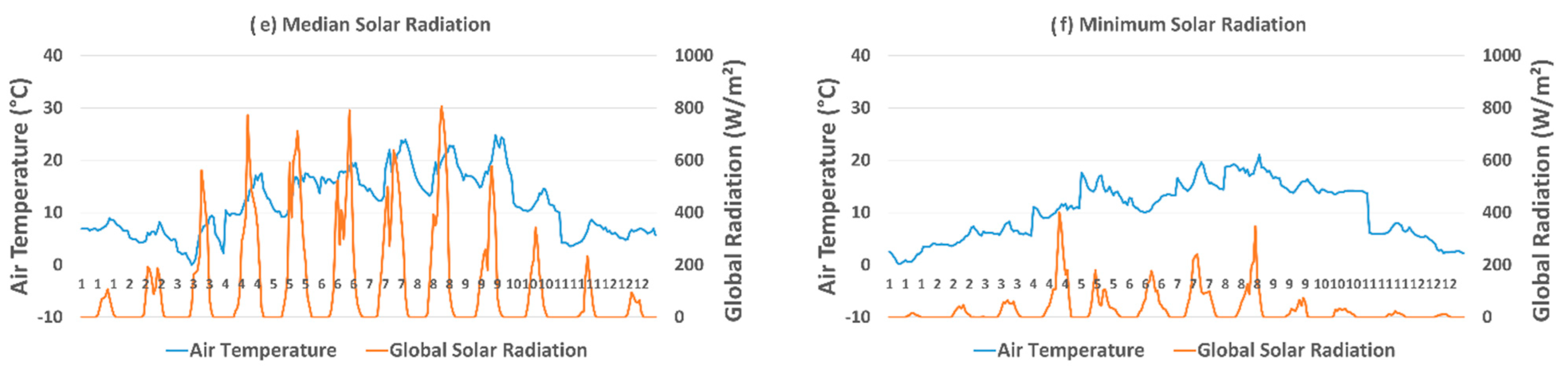
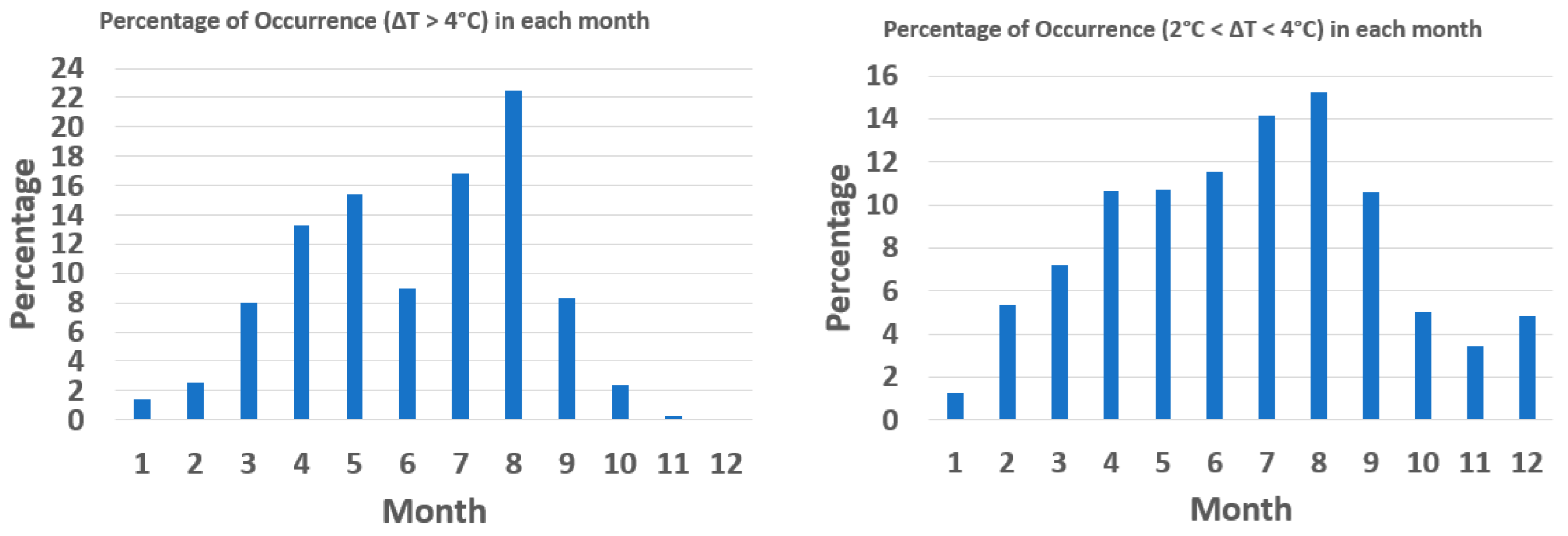
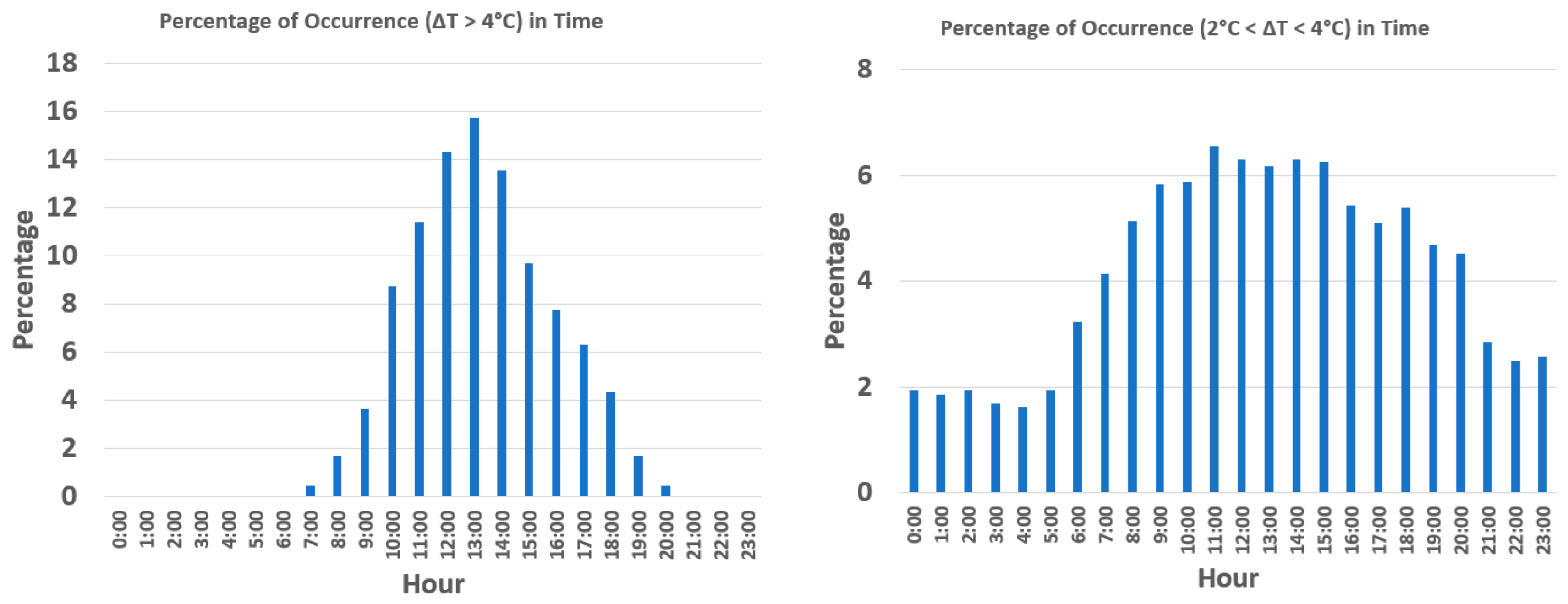
2.2. Representative Days
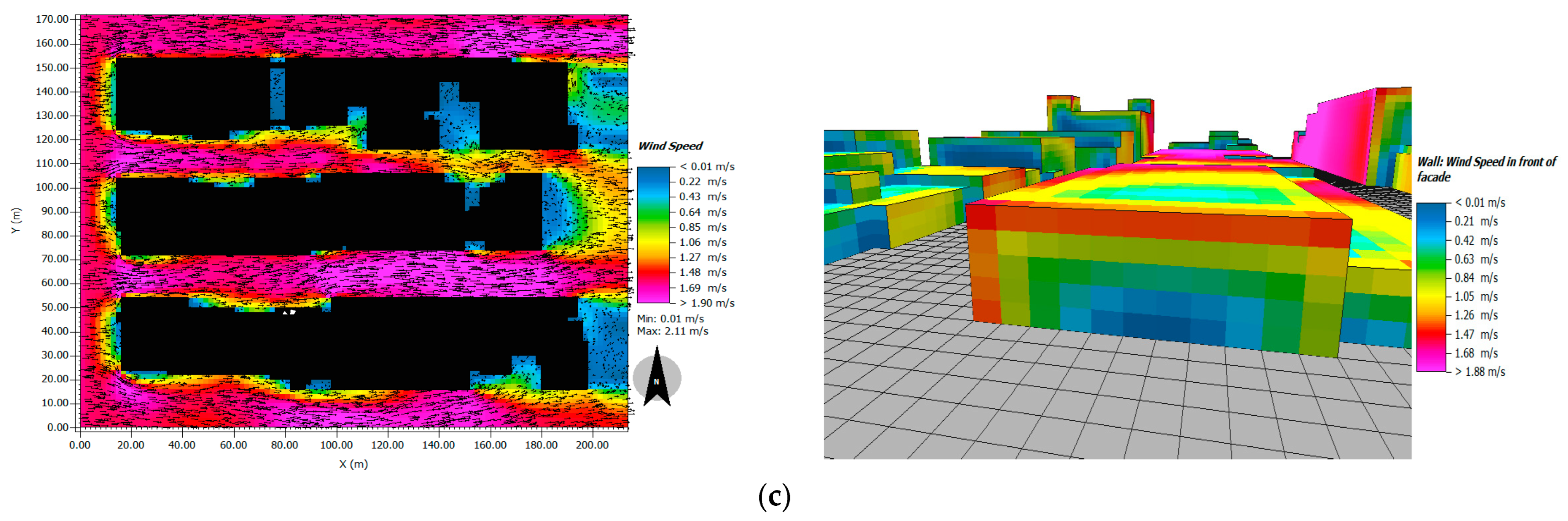
3. Microclimate Modeling (ENVI-met)
3.1. Simulation Setup
3.2. Sensitivity Study
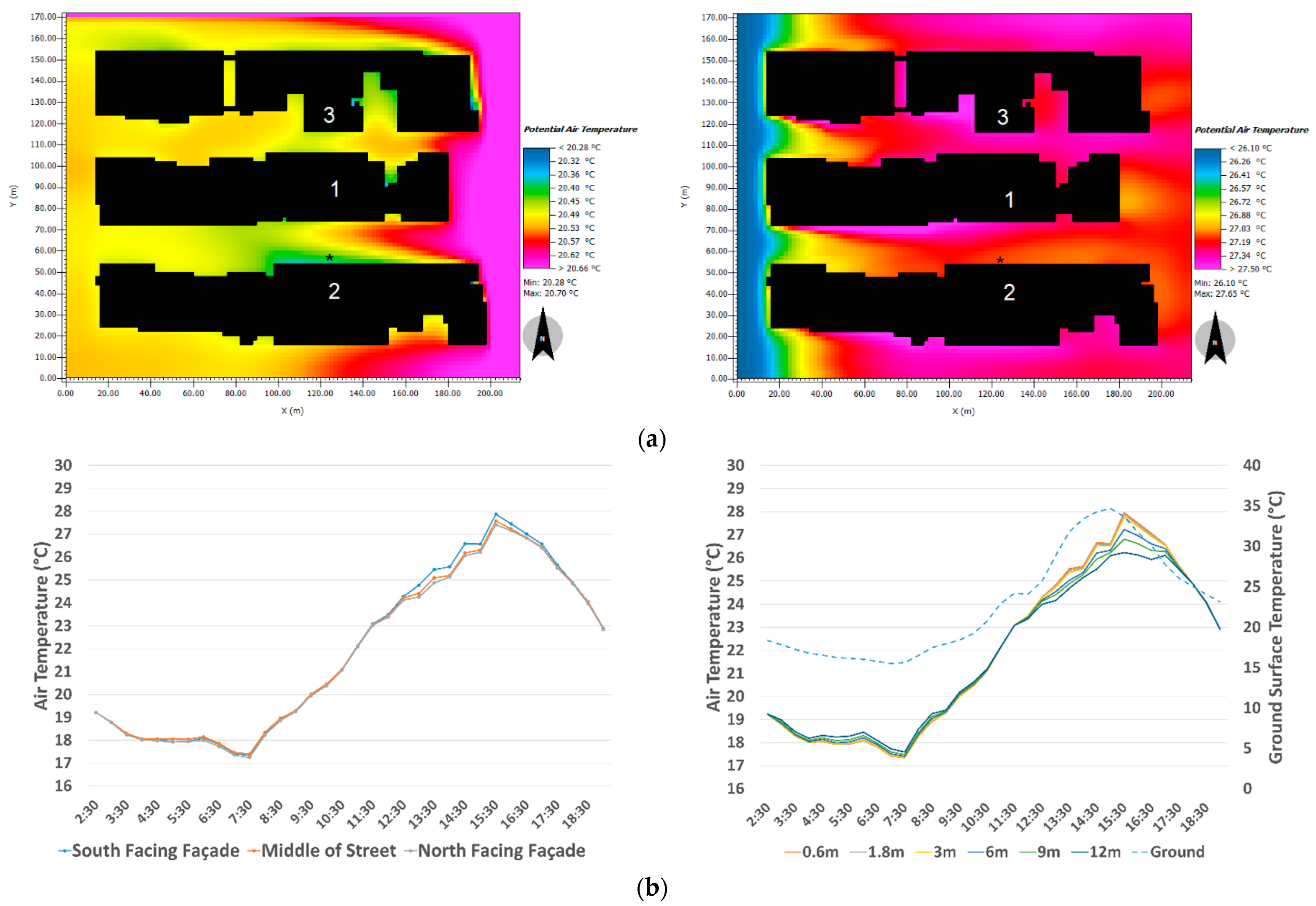
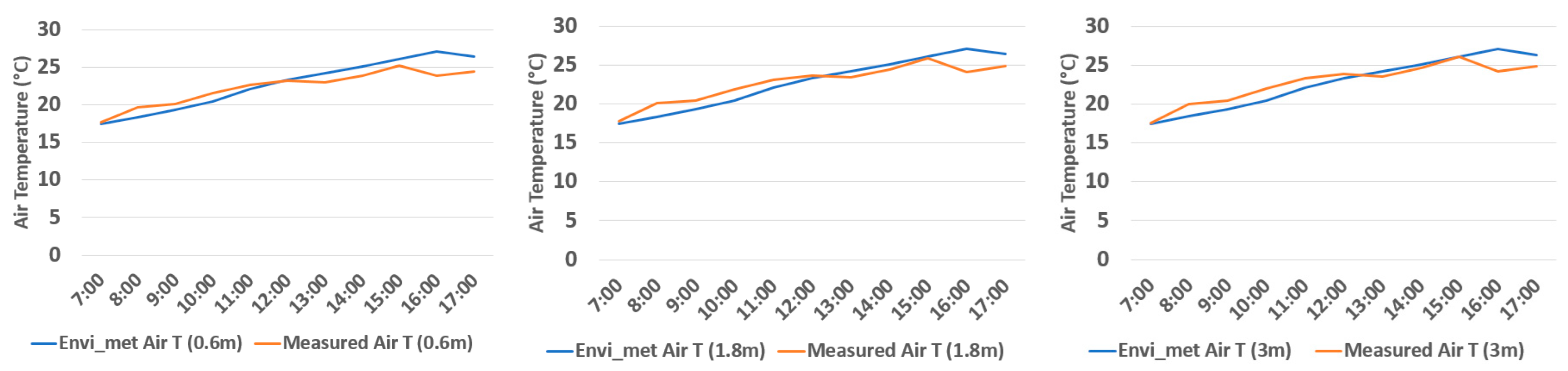
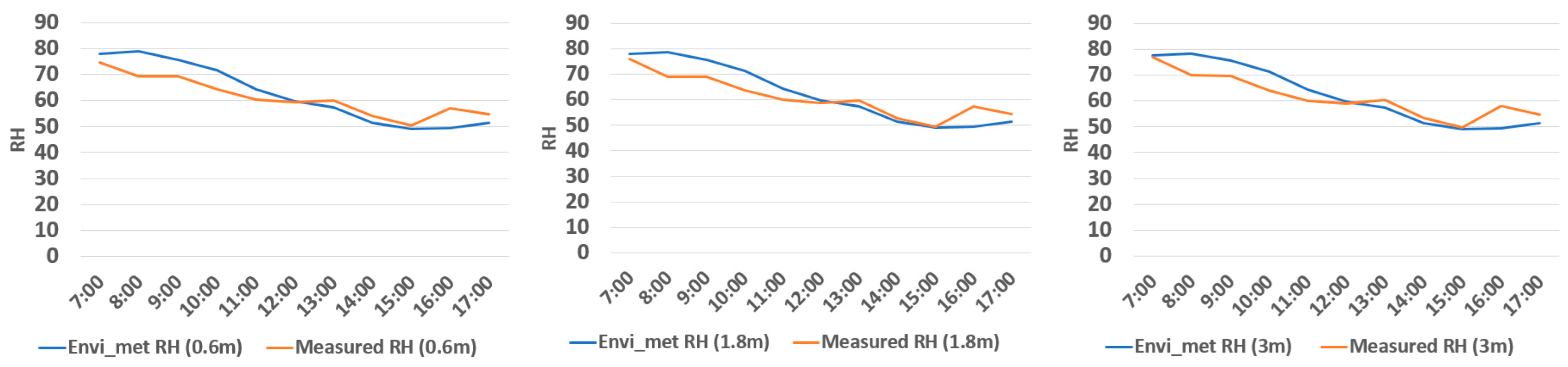
3.3. Validation
4. ANN Models and Urban Canopy Temperature Generation
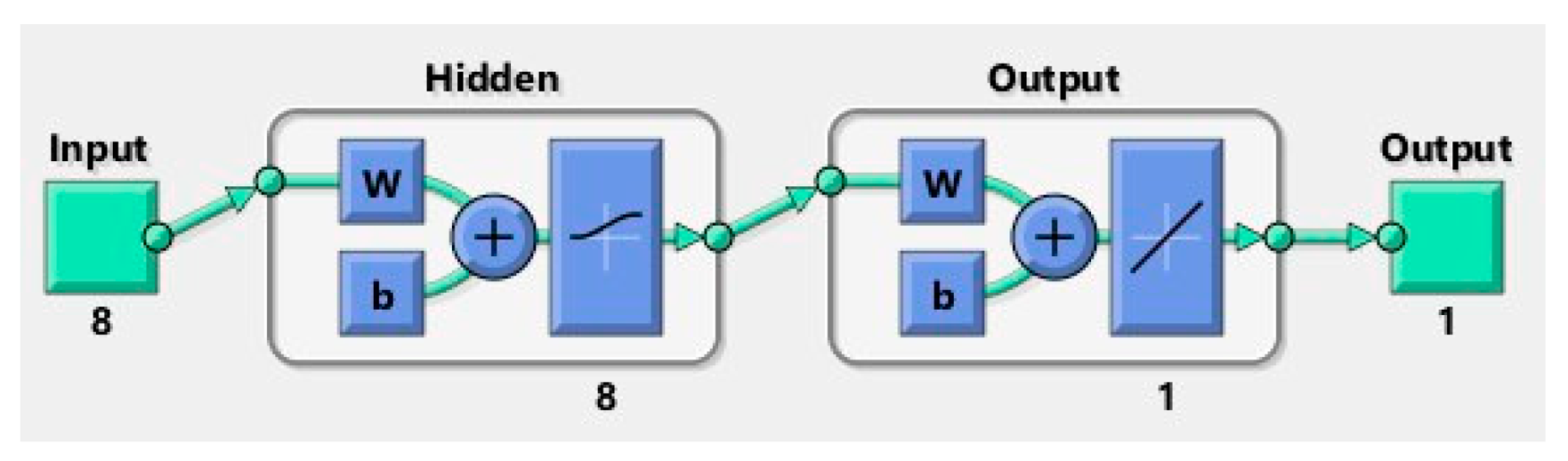
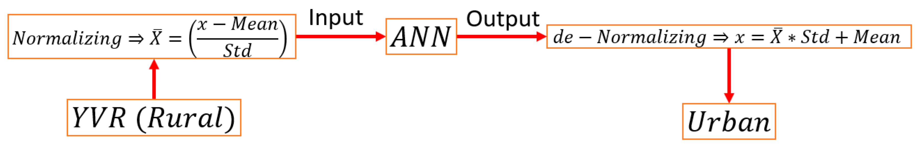
4.1. ANN Models for Urban Air Temperature and Wind Speed Prediction
4.2. Urban Canopy Temperature
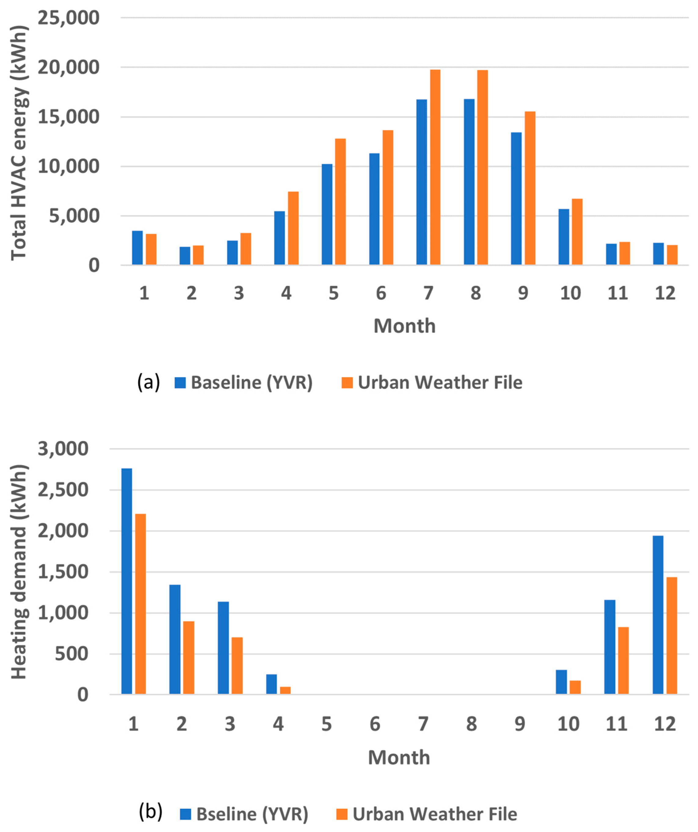
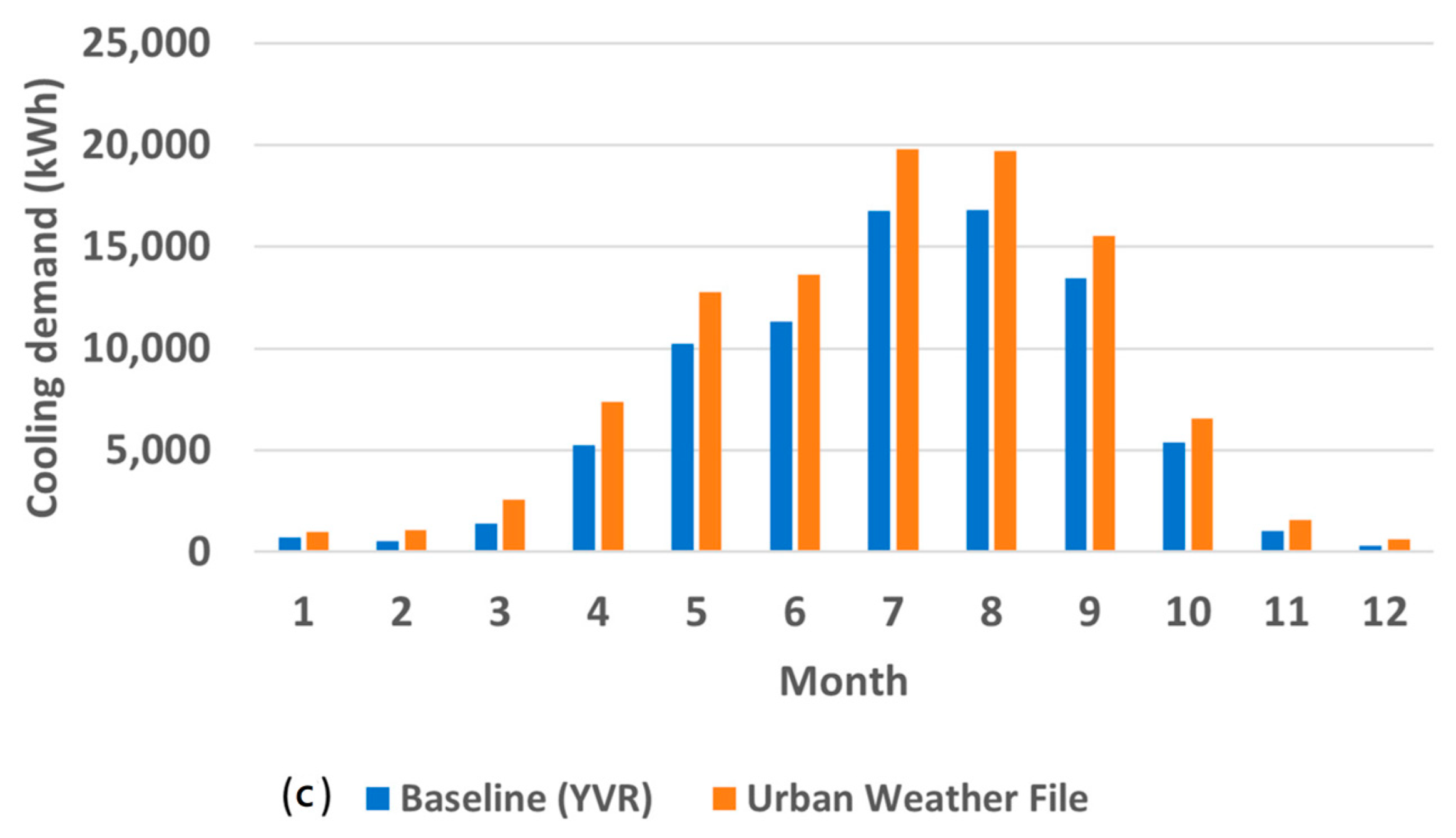
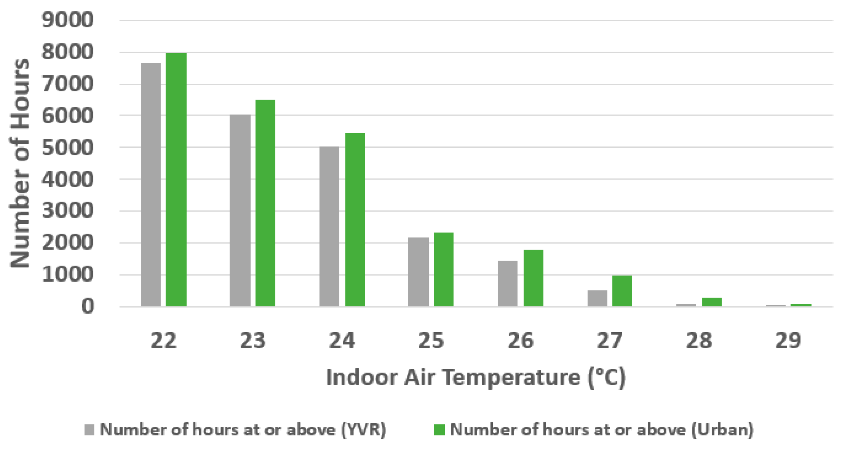
5. Building Energy Consumption for Heating and Cooling with UHI Effect
6. Conclusions
Author Contributions
Funding
Acknowledgments
Conflicts of Interest
References
- Gui, J.; Phelan, P.E.; Kaloush, K.E.; Golden, J.S. Impact of pavement thermophysical properties on surface temperatures. J. Mater. Civ. Eng. 2007, 19, 683–690. [Google Scholar] [CrossRef]
- Yamagata, H.; Nasu, M.; Yoshizawa, M.; Miyamoto, A.; Minamiyama, M. Heat island mitigation using water retentive pavement sprinkled with reclaimed wastewater. Water Sci. Technol. 2008, 57, 763–771. [Google Scholar] [CrossRef] [PubMed]
- Chen, F.; Kusaka, H.; Bornstein, R.; Ching, J.; Grimmond, C.S.B.; Grossman-Clarke, S.; Loridan, T.; Manning, K.W.; Martilli, A.; Miao, S.; et al. The integrated WRF/urban modelling system: Development, evaluation, and applications to urban environmental problems. Int. J. Climatol. 2011, 31, 273–288. [Google Scholar] [CrossRef]
- Li, Y.; Zhao, X. An empirical study of the impact of human activity on long-term temperature change in China: A perspective from energy consumption. J. Geophys. Res. Atmos. 2012, 117, 17117. [Google Scholar] [CrossRef]
- Li, H. Pavement Materials for Heat Island Mitigation: Design and Management Strategies; Butterworth-Heinemann: Oxford, UK, 2015. [Google Scholar]
- Akbari, H. Energy Saving Potentials and Air Quality Benefits of Urban Heat Island Mitigation; Ernest Orlando Lawrence Berkeley National Laboratory: Berkeley, CA, USA, 2005. [Google Scholar]
- Li, X.; Zhou, Y.; Yu, S.; Jia, G.; Li, H.; Li, W. Urban heat island impacts on building energy consumption: A review of approaches and findings. Energy 2019, 174, 407–419. [Google Scholar] [CrossRef]
- Magli, S.; Lodi, C.; Lombroso, L.; Muscio, A.; Teggi, S. Analysis of the urban heat island effects on building energy consumption. Int. J. Energy Environ. Eng. 2015, 6, 91–99. [Google Scholar] [CrossRef]
- Ma, Y.X.; Yu, C. Impact of meteorological factors on high-rise office building energy consumption in Hong Kong: From a spatiotemporal perspective. Energy Build. 2020, 228, 110468. [Google Scholar] [CrossRef]
- Guattari, C.; Evangelisti, L.; Balaras, C.A. On the assessment of urban heat island phenomenon and its effects on building energy performance: A case study of Rome (Italy). Energy Build. 2018, 158, 605–615. [Google Scholar] [CrossRef]
- Liu, Y.; Stouffs, R.; Tablada, A.; Wong, N.H.; Zhang, J. Comparing micro-scale weather data to building energy consumption in Singapore. Energy Build. 2017, 152, 776–791. [Google Scholar] [CrossRef]
- Emamifar, S.; Rahimikhoob, A.; Noroozi, A. Daily mean air temperature estimation from MODIS land surface temperature products based on M5 model tree. Int. J. Climatol. 2013, 33, 3174–3181. [Google Scholar] [CrossRef]
- Ho, H.C.; Knudby, A.; Sirovyak, P.; Xu, Y.; Hodul, M.; Henderson, S.B. Mapping maximum urban air temperature on hot summer days. Remote Sens. Environ. 2014, 154, 38–45. [Google Scholar] [CrossRef]
- Masson, V. A Physically-Based Scheme For The Urban Energy Budget In Atmospheric Models. Bound.-Layer Meteorol. 2000, 94, 357–397. [Google Scholar] [CrossRef]
- Aoyagi, T.; Seino, N. A Square Prism Urban Canopy Scheme for the NHM and Its Evaluation on Summer Conditions in the Tokyo Metropolitan Area, Japan. J. Appl. Meteorol. Climatol. 2011, 50, 1476–1496. [Google Scholar] [CrossRef]
- Kusaka, H.; Kondo, H.; Kikegawa, Y.; Kimura, F. A Simple Single-Layer Urban Canopy Model For Atmospheric Models: Comparison With Multi-Layer And Slab Models. Bound. Layer Meteorol. 2001, 101, 329–358. [Google Scholar] [CrossRef]
- Marciotto, E.R.; Oliveira, A.P.; Hanna, S.R. Modeling study of the aspect ratio influence on urban canopy energy fluxes with a modified wall-canyon energy budget scheme. Build. Environ. 2010, 45, 2497–2505. [Google Scholar] [CrossRef]
- Afshari, A.; Ramirez, N.; Pasha, Y. Increasing the Accuracy of Radiation Heat Transfer Estimation in a Lumped Parameter Urban Canopy Models. Energy Procedia 2019, 158, 5181–5187. [Google Scholar] [CrossRef]
- Bueno, B.; Nakano, A.; Norford, L.; Reinhart, C. Urban Weather Generator—A Novel Workflow for Integrating Urban Heat Island Effect within Urban Design Process. In Proceedings of the 14th Conference of International Building Performance Simulation Association, BS2015. Hyderabad, India, 7–9 December 2015. [Google Scholar]
- Martin, M.; Afshari, A.; Armstrong, P.R.; Norford, L.K. Estimation of urban temperature and humidity using a lumped parameter model coupled with an EnergyPlus model. Energy Build. 2015, 96, 221–235. [Google Scholar] [CrossRef]
- Bueno, B.; Norford, L.; Hidalgo, J.; Pigeon, G. The urban weather generator. J. Build. Perform. Simul. 2012, 6, 269–281. [Google Scholar] [CrossRef]
- Bueno, B.; Norford, L.; Pigeon, G.; Britter, R. A resistance-capacitance network model for the analysis of the interactions between the energy performance of buildings and the urban climate. Build. Environ. 2012, 54, 116–125. [Google Scholar] [CrossRef]
- Bueno, B.; Pigeon, G.; Norford, L.K.; Zibouche, K.; Marchadier, C. Development and evaluation of a building energy model integrated in the TEB scheme. Geosci. Model Dev. 2012, 5, 433–448. [Google Scholar] [CrossRef]
- Allegrini, J.; Dorer, V.; Carmeliet, J. Influence of morphologies on the microclimate in urban neighbourhoods. J. Wind Eng. Ind. Aerodyn. 2015, 144, 108–117. [Google Scholar] [CrossRef]
- Allegrini, J.; Dorer, V.; Carmeliet, J. Coupled CFD, radiation and building energy model for studying heat fluxes in an urban environment with generic building configurations. Sustain. Cities Soc. 2015, 19, 385–394. [Google Scholar] [CrossRef]
- Aboelata, A.; Sodoudi, S. Evaluating urban vegetation scenarios to mitigate urban heat island and reduce buildings’ energy in dense built-up areas in Cairo. Build. Environ. 2019, 166, 106407. [Google Scholar] [CrossRef]
- Castaldo, V.L.; Pisello, A.L.; Piselli, C.; Fabiani, C.; Cotana, F.; Santamouris, M. How outdoor microclimate mitigation affects building thermal-energy performance: A new design-stage method for energy saving in residential near-zero energy settlements in Italy. Renew. Energy 2018, 127, 920–935. [Google Scholar] [CrossRef]
- Fatima, S.; Chaudhry, H. Steady-state CFD modelling and experimental analysis of the local microclimate in Dubai (UAE). Sustain. Build. 2017, 2, 5. [Google Scholar] [CrossRef]
- Toparlar, Y.; Blocken, B.; Maiheu, B.; van Heijst, G.J.F. Impact of urban microclimate on summertime building cooling demand: A parametric analysis for Antwerp 2017, Belgium. Appl. Energy 2018, 228, 852–872. [Google Scholar] [CrossRef]
- Ma, L.; Bo-ot, L.M.; Wang, Y.-H.; Chiang, C.-M.; Lai, C. Effects of a Green Space Layout on the Outdoor Thermal Environment at the Neighborhood Level. Energies 2012, 5, 3723. [Google Scholar] [CrossRef]
- Maragkogiannis, K.; Kolokotsa, D.; Maravelakis, E.; Konstantaras, A. Combining terrestrial laser scanning and computational fluid dynamics for the study of the urban thermal environment. Sustain. Cities Soc. 2014, 13, 207–216. [Google Scholar] [CrossRef]
- Allegrini, J.; Carmeliet, J. Coupled CFD and building energy simulations for studying the impacts of building height topology and buoyancy on local urban microclimates. Urban Clim. 2017, 21, 278–305. [Google Scholar] [CrossRef]
- Allegrini, J.; Carmeliet, J. Simulations of local heat islands in Zürich with coupled CFD and building energy models. Urban Clim. 2018, 24, 340–359. [Google Scholar] [CrossRef]
- Chan, A.L.S. Developing a modified typical meteorological year weather file for Hong Kong taking into account the urban heat island effect. Build. Environ. 2011, 46, 2434–2441. [Google Scholar] [CrossRef]
- Salvati, A.; Coch, H.; Morganti, M. Effects of urban compactness on the building energy performance in Mediterranean climate. Energy Procedia 2017, 122, 499–504. [Google Scholar] [CrossRef]
- Salvati, A.; Coch Roura, H.; Cecere, C. Assessing the urban heat island and its energy impact on residential buildings in Mediterranean climate: Barcelona case study. Energy Build. 2017, 146, 38–54. [Google Scholar] [CrossRef]
- Palme, M.; Inostroza, L.; Villacreses, G.; Lobato-Cordero, A.; Carrasco, C. From urban climate to energy consumption. Enhancing building performance simulation by including the urban heat island effect. Energy Build. 2017, 145, 107–120. [Google Scholar] [CrossRef]
- Litardo, J.; Palme, M.; Borbor-Cordova, M.; Caiza, R.; Macias, J.; Hidalgo-Leon, R.; Soriano, G. Urban Heat Island intensity and buildings’ energy needs in Duran, Ecuador: Simulation studies and proposal of mitigation strategies. Sustain. Cities Soc. 2020, 62, 102387. [Google Scholar] [CrossRef]
- Bruse, M.; Fleer, H. Simulating surface–plant–air interactions inside urban environments with a three dimensional numerical model. Environ. Model. Softw. 1998, 13, 373–384. [Google Scholar] [CrossRef]
- Simon, H.; Bruse, M.; Kissel, L. Evaluation of ENVI-Met’s Multiple-Node Model and Estimation of Indoor Climate. Available online: https://www.researchgate.net/publication/318561953_Evaluation_of_ENVI-met’s_multiple-node_model_and_estimation_of_indoor_climate (accessed on 14 May 2023).
- Awol, D.A.; Bitsuamlak, G.T.; Tariku, F. Numerical estimation of the external convective heat transfer coefficient for buildings in an urban-like setting. Build. Environ. 2020, 169, 106557. [Google Scholar] [CrossRef]
- Kahsay, M.; Bitsuamlak, G.T.; Tariku, F. Effect of localized exterior convective heat transfer on high-rise building energy consumption. Build. Simul. J. 2020, 13, 127–139. [Google Scholar] [CrossRef]
- Tsoka, S.; Tsikaloudaki, A.; Theodosiou, T. Analyzing the ENVI-met microclimate model’s performance and assessing cool materials and urban vegetation applications—A review. Sustain. Cities Soc. 2018, 43, 55–76. [Google Scholar] [CrossRef]
- Mohandes, S.R.; Zhang, X.; Mahdiyar, A. A comprehensive review on the application of artificial neural networks in building energy analysis. Neurocomputing 2019, 340, 55–75. [Google Scholar] [CrossRef]
- Dong, Q.; Xing, K.; Zhang, H. Artificial Neural Network for Assessment of Energy Consumption and Cost for Cross Laminated Timber Office Building in Severe Cold Regions. Sustainability 2018, 10, 84. [Google Scholar] [CrossRef]
- Şahin, M. Modelling of air temperature using remote sensing and artificial neural network in Turkey. Adv. Space Res. 2012, 50, 973–985. [Google Scholar] [CrossRef]
- Schuch, F.; Marpu, P.; Masri, D.; Afshari, A. Estimation of Urban Air Temperature From a Rural Station Using Remotely Sensed Thermal Infrared Data. Energy Procedia 2017, 143, 519–525. [Google Scholar] [CrossRef]


| Researcher Location | Urban Weather Data Determination Method | Building Energy Simulation Software | Duration | Findings and Variables |
|---|---|---|---|---|
| Chan (2011) [34] Hong Kong | Field Measurements | EnergyPlus | 6 months | 10% cooling energy increase with UHII of 1.4 °C |
| Salvati et al. (2017) [35,36] Barcelona | Field Measurements | EnergyPlus | 3 days | 18–28% cooling energy increase with UHII of 2.8 °C in winter and 1.7 °C in summer |
| Liu et al. (2017) [11] Singapore | Field Measurements | EnergyPlus | Whole year | 7% average cooling energy increase with UHII of 1–2 °C |
| Ma and Yu (2020) [9] Hong Kong | Field Measurements | EnergyPlus | Whole year | 8% and 3% summer and winter energy consumption increase by every 1 °C |
| Magli et al. (2015) [8] Italy | Field Measurement | TRNSYS | Whole year | 8% cooling energy increase, 20% heating energy decrease, and 7% CO2 emission increase by UHII of 1.4 °C |
| Guattari et al. (2018) [10] Italy | Field Measurement | TRNSYS | Whole year | 30% cooling energy increase and 11% heating energy decrease by UHII of 1.4 °C at night and 0.84 °C during the daytime |
| Palme et al. (2017) [37] South America | Urban Weather Generator | TRNSYS | Whole year | 15% to 200% cooling energy increase by different UHII |
| Litardo et al. (2020) [38] Ecuador | Urban Weather Generator | TRNSYS | Whole year | 30% to 70% cooling energy increase for residential by UHII of 0.6 °C in September and 1.25 °C in February |
| Castaldo et al. (2018) [27] Italy | ENVI-met and Meteonorm | EnergyPlus | July 19 and January 3 | 10% HVAC energy reduction by 1.5 °C reduction in air temperature in summer |
| Aboelata and Sodoudi (2019) [26] Egypt | ENVI-met | DesignBuilder | 24 h | 4% (1.252 Euros/day) cooling energy decrease by 1 °C reduction in air temperature by adding 50% trees |
| Toparlar et al. (2018) [29] Belgium | ANSYS Fluent | EnergyPlus | 1 month (July) | 90% cooling energy increase in July by UHII of 3.3 °C |
| Fatima and Chaudhry (2017) [28] Dubai | ANSYS Fluent | Newton’s law of cooling | 1 h | 19% cooling energy increase for every 1.22 °C temperature rise |
| Months | T_Max | T_Ave | T_Min | Rad_Max | Rad_Ave | Rad_Min |
|---|---|---|---|---|---|---|
| January | 3 | 22 | 14 | 28 | 25 | 10 |
| February | 20 | 12 | 4 | 24 | 16 | 7 |
| March | 21 | 12 | 2 | 15 | 8 | 5 |
| April | 16 | 12 | 3 | 18 | 23 | 22 |
| May | 28 | 12 | 2 | 27 | 1 | 30 |
| June | 23 | 11 | 15 | 7 | 27 | 9 |
| July | 21 | 17 | 1 | 18 | 13 | 11 |
| August | 16 | 10 | 7 | 4 | 25 | 21 |
| September | 10 | 22 | 26 | 3 | 2 | 23 |
| October | 2 | 16 | 23 | 3 | 17 | 9 |
| November | 2 | 6 | 9 | 1 | 13 | 24 |
| December | 5 | 12 | 29 | 2 | 10 | 21 |
| Air T | ||
| Height | Mean Absolute Error | Root Mean Square Error |
| Overall: | MAE: 1.1 °C | RMSE:1.35 °C |
| 0.6 m: | MAE: 1.15 °C | RMSE:1.41 °C |
| 1.8 m: | MAE: 1.1 °C | RMSE:1.34 °C |
| 3 m | MAE: 1.05 °C | RMSE:1.31 °C |
| RH | ||
| Overall: | MAE: 4.17% | RMSE: 5.12% |
| 0.6 m: | MAE: 4.39% | RMSE: 5.2% |
| 1.8 m: | MAE: 4.14% | RMSE: 5.18% |
| 3 m | MAE: 4% | RMSE: 4.96% |
| Applied ANN Features | |
|---|---|
| Network Type: | Feed-forward backpropagation |
| Training Function: | Levenberg–Marquardt (Trainlm) |
| Performance Function: | RMSE |
| Number of Hidden Layers: | 1 |
| Activation Function: | logsig (hidden layer) and Purelin (output) |
| Number of Neurons in Hidden Layer | ||||||
|---|---|---|---|---|---|---|
| Runs | 1 | 8 | 15 | 17 | 20 | 100 |
| 1 | 1.2904 | 1.2121 | 1.2171 | 1.2219 | 1.2350 | 1.4055 |
| 2 | 1.2930 | 1.2190 | 1.2201 | 1.2284 | 1.2319 | 1.5064 |
| 3 | 1.2693 | 1.2170 | 1.2190 | 1.2181 | 1.2399 | 1.4118 |
| 4 | 1.2815 | 1.2191 | 1.2195 | 1.2201 | 1.2339 | 1.6395 |
| 5 | 1.2721 | 1.2184 | 1.2190 | 1.2174 | 1.2460 | 1.5508 |
| Material | Property | |||
|---|---|---|---|---|
| Thickness (m) | Density (Kg/m3) | Conductivity (W/mK) | Specific Heat (J/KgK) | |
| XPS | 0.18 | 35 | 0.034 | 1400 |
| Concrete | 0.18 and 0.1 | 2220 | 1.6 | 850 |
| EPS | 0.07 and 0.147 | 15 | 0.04 | 1400 |
| Plaster | 0.01 | 1500 | 0.6 | 850 |
| Ceramic Tile | 0.03 | 1700 | 0.8 | 850 |
| Percentage of Change (UHI Affected—Baseline (YVR)) | |
|---|---|
| Total Heating: | −29% (−1.08 kWh/m2) |
| Total Cooling: | 23% (8.09 kWh/m2) |
| Total Energy: | 18% (7.01 kWh/m2) |
Disclaimer/Publisher’s Note: The statements, opinions and data contained in all publications are solely those of the individual author(s) and contributor(s) and not of MDPI and/or the editor(s). MDPI and/or the editor(s) disclaim responsibility for any injury to people or property resulting from any ideas, methods, instructions or products referred to in the content. |
© 2023 by the authors. Licensee MDPI, Basel, Switzerland. This article is an open access article distributed under the terms and conditions of the Creative Commons Attribution (CC BY) license (https://creativecommons.org/licenses/by/4.0/).
Share and Cite
Tariku, F.; Gharib Mombeni, A. ANN-Based Method for Urban Canopy Temperature Prediction and Building Energy Simulation with Urban Heat Island Effect in Consideration. Energies 2023, 16, 5335. https://doi.org/10.3390/en16145335
Tariku F, Gharib Mombeni A. ANN-Based Method for Urban Canopy Temperature Prediction and Building Energy Simulation with Urban Heat Island Effect in Consideration. Energies. 2023; 16(14):5335. https://doi.org/10.3390/en16145335
Chicago/Turabian StyleTariku, Fitsum, and Afshin Gharib Mombeni. 2023. "ANN-Based Method for Urban Canopy Temperature Prediction and Building Energy Simulation with Urban Heat Island Effect in Consideration" Energies 16, no. 14: 5335. https://doi.org/10.3390/en16145335
APA StyleTariku, F., & Gharib Mombeni, A. (2023). ANN-Based Method for Urban Canopy Temperature Prediction and Building Energy Simulation with Urban Heat Island Effect in Consideration. Energies, 16(14), 5335. https://doi.org/10.3390/en16145335