1. Introduction
With the aim of ensuring that EU policies are in line with the climate goals agreed by the Council and the European Parliament, the Fit for 55 [
1] package was proposed, which among other things, includes an increase in the CO
2eq emissions from the buildings reduction target by 2030 compared to 2005. The measures include, among others, enhancing buildings’ energy performance when constructing new buildings and the energy renovation of existing buildings. All of this also complies with the European Commission’s long-term strategy for a low-carbon Europe by 2050 [
2,
3]. The European parliament adopted draft measures to increase the building renovation rate as well as to minimize buildings’ energy consumption and CO
2eq emissions. European Climate Law [
4] enshrined both the 2030 and the 2050 targets into binding European law. According to the adopted measures, all new buildings should be zero-emission buildings (ZEBs) from 2028, while new buildings occupied, operated or owned by public authorities should be from 2026 [
5], thus advancing even further the development set up by nearly zero energy buildings (NZEBs).
To achieve these goals, it is important to predict the energy consumption of both new buildings and renovated buildings. Most software used in the EU for energy performance simulation use simplified methods to calculate heat transfer through building elements based on steady-state boundary conditions averaged over a period of time [
6,
7]. This calculation can lead to unsatisfactory results when boundary conditions change rapidly and when the thermal mass of the element is significant [
6,
8]. As a result, the predicted energy demand may be lower or higher than the actual energy consumption, leading to undersized or oversized heating and cooling systems. Furthermore, if the boundary conditions are considered to be steady-state, the peak energy demand shifts because the thermal mass is not taken into account, leading to a thermal comfort problem for the building occupants. Nowadays, dynamic methods for simulating building energy demand are more and more widely used because they are powerful and important tools for optimizing building energy demand [
8,
9,
10,
11,
12].
The dynamic methods are based on the non-stationary solution of the heat equation. This solution can be found numerically (finite volume method, finite element method or finite difference method) or analytically. Due to the long analysis period and small time steps used for the analysis, numerical methods have proven to be inadequate for building energy simulations because they rely on solving large systems of equations at each time step [
13]. Analytical methods such as conduction transfer functions (CTFs) have been shown to be much better for building energy simulation problems [
14] and are implemented in modern dynamic energy simulation software such as TRNSYS [
15] and EnergyPlus [
16]. Although the CTF methods are superior to the abovementioned simplified calculations, the aim of this research is to show that they have their limitations and lead to unsatisfactory results if not properly applied. It will be shown that in the case of heavyweight façade systems and small computational time steps, CTFs can provide low-quality results (become more and more unstable with longer time steps, particularly with massive building elements) [
17]. The reason for using small time steps, which in some cases can be less than one hour, could be to analyze more accurately the impact of complex control systems on the overall energy performance of the building primarily associated with the exploitation of renewable energy sources as well as predictive model control of buildings [
18,
19]. Another reason is that NZEBs and ZEBs require more accurate dynamic simulations of heavy and highly insulated building elements with shorter time steps (less than 15 min) [
20,
21,
22]. The problem also lies in the algorithms developed for yearly energy simulations with a time step of one hour. Comparisons of different methods and their main problems found in the literature are summarized in
Table 1.
Among the most commonly used CTF methods are the Laplace method and the State-Space method. This paper compares these two methods for calculating heat losses through a heavyweight multilayer wall with a contact thermal insulation façade system by implementing the algorithms from the research work of Stephenson and Mitalas [
23] for the Laplace method and Seem [
24] for the State-Space method in Mathematica [
25]. The software Mathematica was chosen due to its advanced mathematical and numerical tools and matrix manipulation. The results from Mathematica are then compared with the results of two commonly used software for the dynamic calculation of energy performance—TRNSYS and EnergyPlus. The first software uses the Laplace method [
21,
26] to calculate the CTF coefficients, while the second uses the State-Space method [
27,
28,
29]. The finite difference method (FDM) [
30] is used as a reference point for the boundary heat flux density. The aim is to show how well the Laplace method and the State-Space method perform for small time steps and heavyweight building elements and what possibilities there are for improving these methods.
2. Methodology
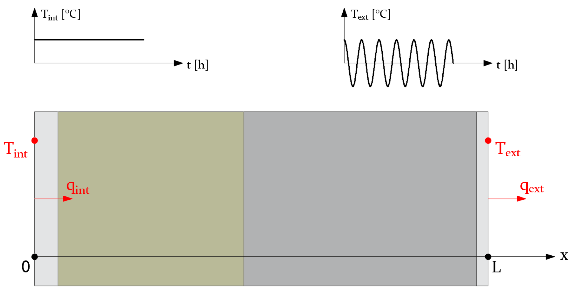
If we consider a multilayer wall, as shown in
Figure 1, in the general case, the wall is composed of n layers and two boundary conditions. The boundary condition for x = 0 is T
int and for x = L T
ext. For the building energy performance simulation, the surface heat fluxes on the interior (q
int) and the exterior (q
ext) surface must be calculated since these two fluxes represent the energy demand for the element under consideration. Only heat flux due to conduction is considered and boundary conditions are surface temperatures on the internal and external surfaces. Convection and radiation on both surfaces are not considered, i.e., R
si and R
se are taken as 0 (m
2 K)/W. Solar radiation as well as all other radiation from the environment is not taken into account for the calculation. This assumption simplifies the calculation of the surface heat fluxes and the implementation of the Steady-State and Laplace method algorithms in Mathematica. The same assumption is implemented in both Mathematica’s algorithms, EnergyPlus and TRNSYS.
In most cases, heat transfer through building elements such as walls or ceilings can be considered one-dimensional. The heat equation for one-dimensional heat conduction is given by Equation (1).
With the boundary and initial conditions:
where
T(
x,
t) is the temperature at point x at time t in °C,
λ is the thermal conductivity in W/(m K),
is the density in kg/m
3,
cp is the specific heat in J/(kg K),
Tint is the internal surface temperature in °C,
Text is the external surface temperature in °C,
qint is the internal surface heat flux in W/m
2 and
qext is the external surface heat flux in W/m
2.
In this research, Equation (1) is solved using:
The State-Space method [
24];
The finite difference method;
The State-Space method, as implemented in EnergyPlus;
The Laplace method, as implemented in TRNSYS.
For the solution of each method, the internal surface heat flux is calculated. The solution for all five methods is then compared to analyse the impact of each method on the solution, and also to analyse the efficiency of each algorithm used by the abovementioned methods. This analysis is performed for time steps ranging from one hour to six minutes and for lightweight and heavyweight building elements (walls). As a reference solution for the comparison (i.e., as the exact solution), the solution of the FDM is taken. Furthermore, the steady-state solution is calculated to show the difference between the transient (dynamic) and steady-state building energy demand simulation.
2.1. The Finite Difference Method
The finite difference method (FDM) is a method used for obtaining a numerical solution to Equation (1). As with most numerical solutions, the FDM uses a discrete approximation of the continuous partial differential equation. This means that the solution is known only at a finite number of points within the element. The number of these points is user-defined and generally increases the accuracy of the numerical solution. The discrete approximation of Equation (1) is as follows [
31]:
Equation (3) represents the implicit FDM formulation for solving the heat equation. In the matrix formulation, Equation (3) can be written as follows:
The subscript
i denotes a node and
j point in time. The coefficients
r1 and
r2 are calculated for each node according to Equation (5).
By solving Equation (4) for each time step
j, the internal heat flux
qint can be calculated using Fourier’s law of thermal conduction as follows:
The solution calculated using Equation (6) is used as a reference (i.e., as an exact solution) for the comparison.
2.2. The State-Space Method
The State-Space method is usually used to describe a linear system with r inputs, m outputs and n state variables that are written in the general form as described in [
32]:
Here
x is the state vector,
u is the input vector,
y is the output vector,
t is time, and
A,
B,
C and
D are matrices of dimension n × n, n × r, m × n and m × r, respectively. Since, in the case of heat conduction, the system is time-variant (i.e., the temperature inside the element changes with time), Equations (7) and (8) can be written by discrete time-variant State-Space method as in [
32]:
Here the matrices
A,
B,
C and
D have the same dimensions as in the continuous time case—Equations (7) and (8). In the case of heat conduction, the state vector
x represents the temperatures of each node of the element, the input vector
u represents the boundary conditions (i.e., the boundary temperatures shown in
Figure 1) and the output vector
y represents the surface heat fluxes
qi and
qe shown in
Figure 1.
Equations (9) and (10) can be used to solve Equation (1) by enforcing the finite difference grid over the analysed building element:
The coefficients
r1 and
r2, which represent the left node “
i − 1” and the node “
i” for each row of the matrix, are calculated for each node using Equation (12).
where index “
i” denotes the node in the FDM grid (
i = 2 to n) and “
i − 1” first previous node in the FDM grid.
The interior heat flux can be written in the matrix form as follows:
If Equations (11) and (13) are compared to Equations (9) and (10), then matrices
A,
B,
C and
D are equal to:
The matrices (14) are the input values for the algorithm [
24] to calculate the CTF coefficients
Zj,
Yj and
φj. The algorithm [
24] is implemented in Mathematica [
25], and all operations with matrices were performed using this powerful software. From the CTF coefficients, the interior heat flux is calculated as follows:
where
Zj is the interior CTF coefficient,
Yj is the cross CTF coefficient and
φj is the flux CTF coefficient.
NZ,
NY and
Nφ represent the number of
Zj,
Yj and
φj coefficients, respectively.
It is common practice to use Equation (16) to verify that the CTF coefficients obtained by the State-Space method give the correct steady-state heat transfer, with
Xk being the exterior CTF coefficient.
2.3. The Laplace Method
The Laplace method uses Laplace transforms to solve Equation (1) [
33]. In matrix form, this solution can be written as follows:
Here AA(s), BB(s), CC(s) and DD(s) are the elements of the wall transmission matrix H that relates to the surface temperatures and surface heat flux, with NL being the number of layers, s being the frequency in the Laplace domain, and Lk and α being the thickness and the thermal diffusivity of each layer, respectively.
For the purpose of building performance simulation, and because DD(s) = AA(s), Equation (17) is transformed into Equation (18) [
34].
In their work, [
23] introduced a procedure that uses Z-Transforms [
35] to convert the solution from the frequency domain (s) back to the time domain (t). This procedure is based on the partial fraction expansion [
36,
37] and finding roots of the denominator BB(s) on some predefined interval. The root-finding algorithm is one of the main drawbacks of the Laplace method, as it can lead to an excessive computation time and potential calculation errors [
38]. Although the Laplace method is an analytical method, except for the root-finding procedure, which is mostly conducted numerically, the State-Space method has been shown to be superior for shorter time steps and heavyweight building elements [
39,
40]. Some researchers have tried to overcome the problem of root-finding such as [
41], which proved to be efficient. They discovered that the roots of the heat transfer function BB(s) are separated by the roots of the transfer function AA(s). This new discovery ensured that no roots of the heat transfer function BB(s) are overlooked when performing the root-finding procedure. Nevertheless, they did not overcome the problem of using numerical methods for finding the actual roots, which was performed by the classical bisection method. In this paper, the root-finding procedure is performed using Mathematica’s
FindRoot function and Brent’s method [
42], in contrast to TRNSYS, which uses the bisection method.
From the CTF coefficients (
bj,
cj,
dj), the interior heat flux is calculated as follows:
where
bj is the interior CTF coefficient,
cj is the cross CTF coefficient and
dj is the flux CTF coefficient.
Nb,
Nc and
Nd represent the number of
bj,
cj and
dj coefficients, respectively.
It is common practice to use Equation (20) to verify that the CTF coefficients obtained by the Laplace method give the correct steady-state heat transfer.
2.4. EnergyPlus
Version of the software used in this research is version 9.6. The building elements were modelled in a single zone environment and only heat conduction through the wall was considered, i.e., convection and radiation on both internal and external surface were set to zero in EnergyPlus settings. That means that the temperature on of the internal and external surface was the same as the air temperature. EnergyPlus uses Steady-State method for the approximation of the solution for the heat equation as shown below. The same weather file used in Mathematica was also used in EnergyPlus.
The following equation shows the basic form of a CTF solution for the internal surface heat flux [
43]:
where
Zj is the interior CTF coefficient,
Yj is the cross CTF coefficient and
φj is the flux CTF coefficient.
NZ,
NY and
Nφ represent the number of
Zj,
Yj and
φj coefficients, respectively.
2.5. Trnsys
Version of the software used in this research is 17. For consistency with both EnergyPlus and algorithms implemented in Mathematica for Steady-State and Laplace method algorithms, only conduction through the wall was modelled. Convection and radiation on the internal and external surface were not considered. The temperature of the internal surface was the same as the air temperature. The building element was also modelled in a single zone environment. The same weather file that was used in Mathematica was used in TRNSYS.
The instantaneous heat flux entering or leaving the zone for an exterior wall can be modelled according to Equation (19) as described in [
44].
3. Results
In this section, the results of all the abovementioned methods are compared to check the efficiency of each method for different time steps and two types of building elements (i.e., heavyweight and lightweight) shown in
Table 2 and
Table 3. The time steps used for the analysis were 1 h, 0.5 h, 0.25 h and 0.1 h. The thermal transmittance (U-value) of each building element was also calculated to determine the steady-state surface heat flux as:
The U-value in this research refers to surface-to-surface heat conduction that does not take into account the values of the surface heat transfer resistances due to the convection and radiation, i.e., R
si = 0 (m
2 K)/W and R
se = 0 (m
2 K)/W. U-values calculated this way cannot be used as the design values. If the design values are to be calculated from the material properties and thicknesses shown in
Table 2 and
Table 3, then the procedure and values of the surface heat transfer coefficients (h
si and h
se) given by ISO 6946 standard are to be used accordingly.
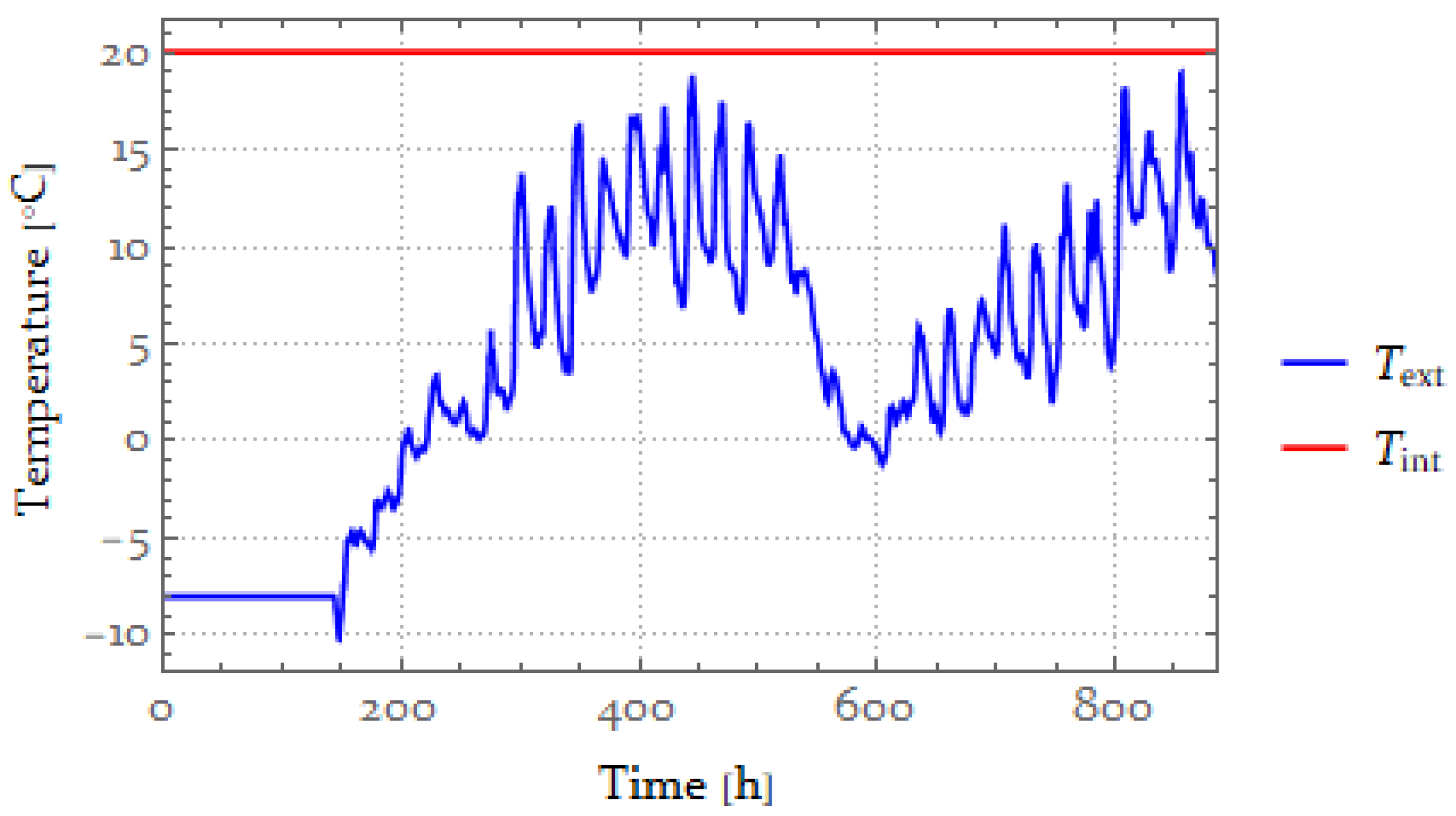
The boundary conditions used for the analysis were 20 °C for the interior surface temperature (T
int), and the values for the exterior surface temperatures (T
ext) were taken from [
45] for the City of Zagreb (
Figure 2). The data taken from [
45] provide climate data with a 30 min time step, and to be able to use it for shorter time steps, the data are transformed into a continuous function using Mathematica’s algorithms. The calculation period was one month, with a warm-up period of six days to neutralize the effects of the initial conditions. Since only heat conduction through the elements was considered, the internal and external surface heat transfer coefficients were both taken as 0 W/(m
2 K).
To check the stability of the results, Equations (16) and (20) are used (
Table 4 and
Table 5).
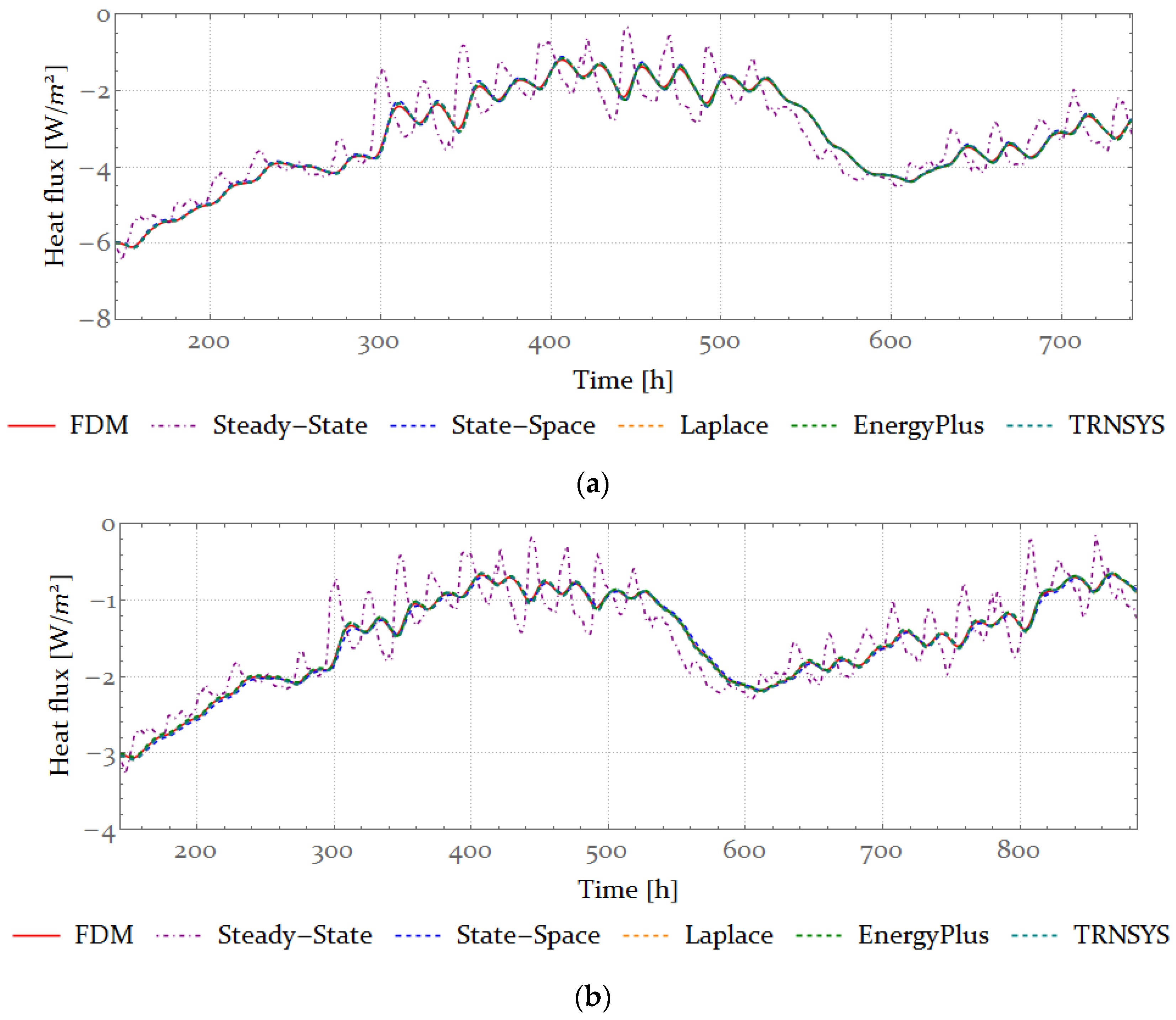
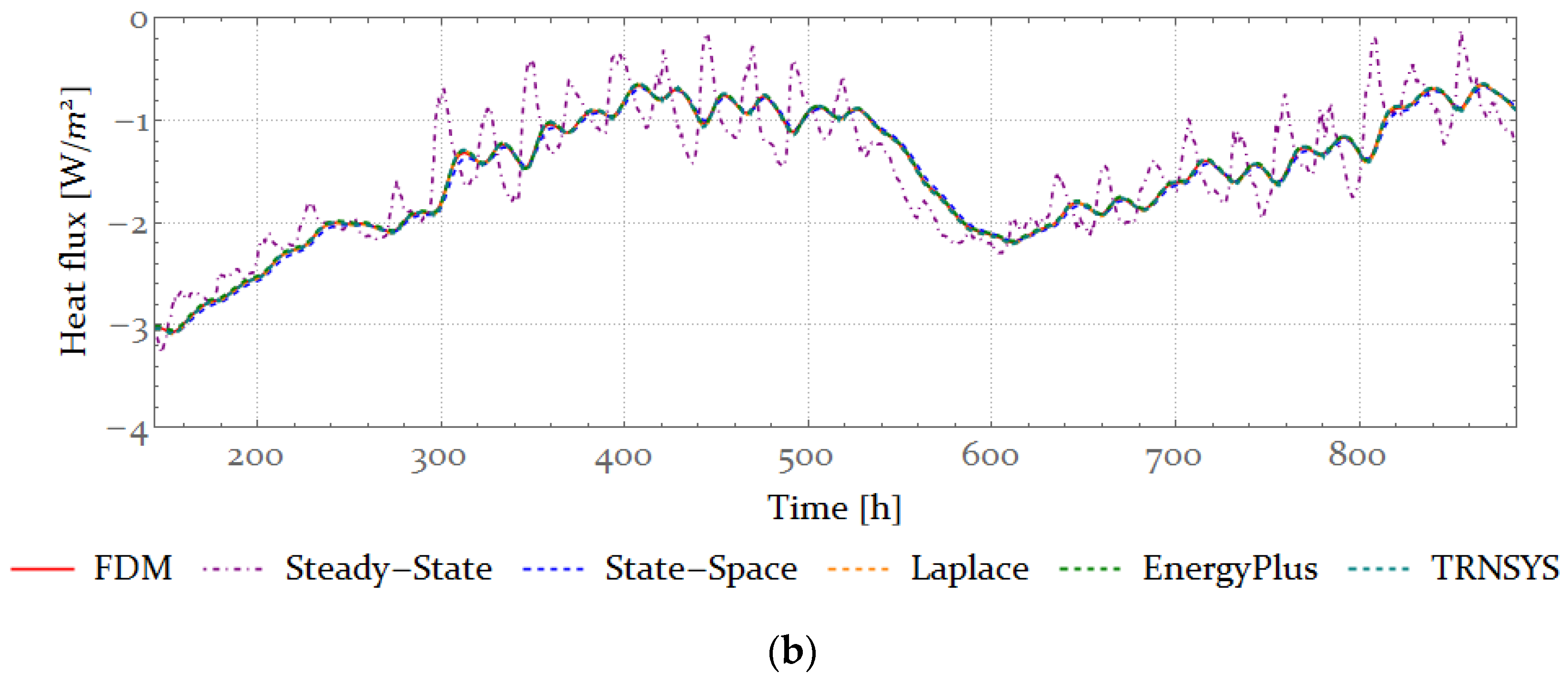
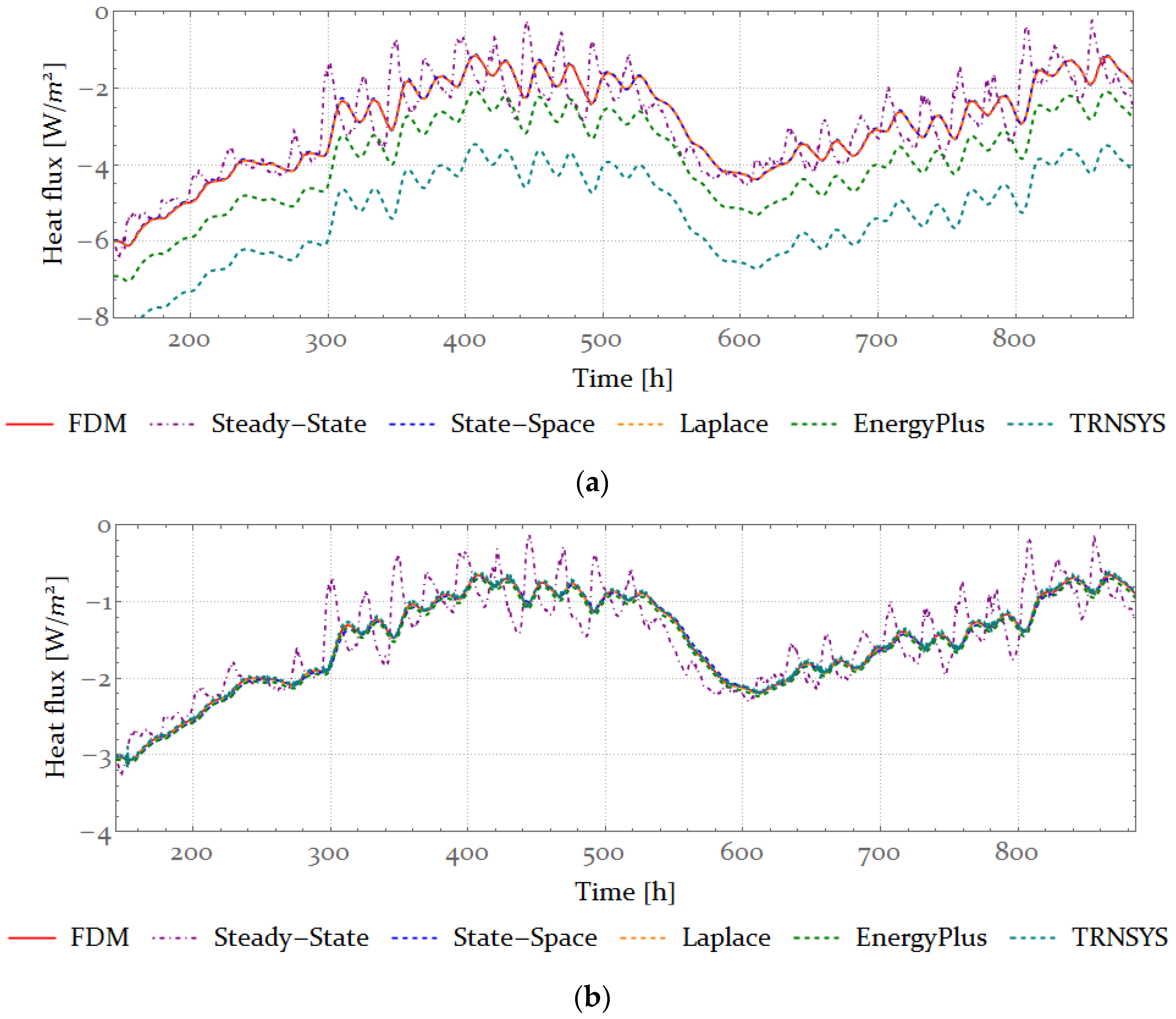
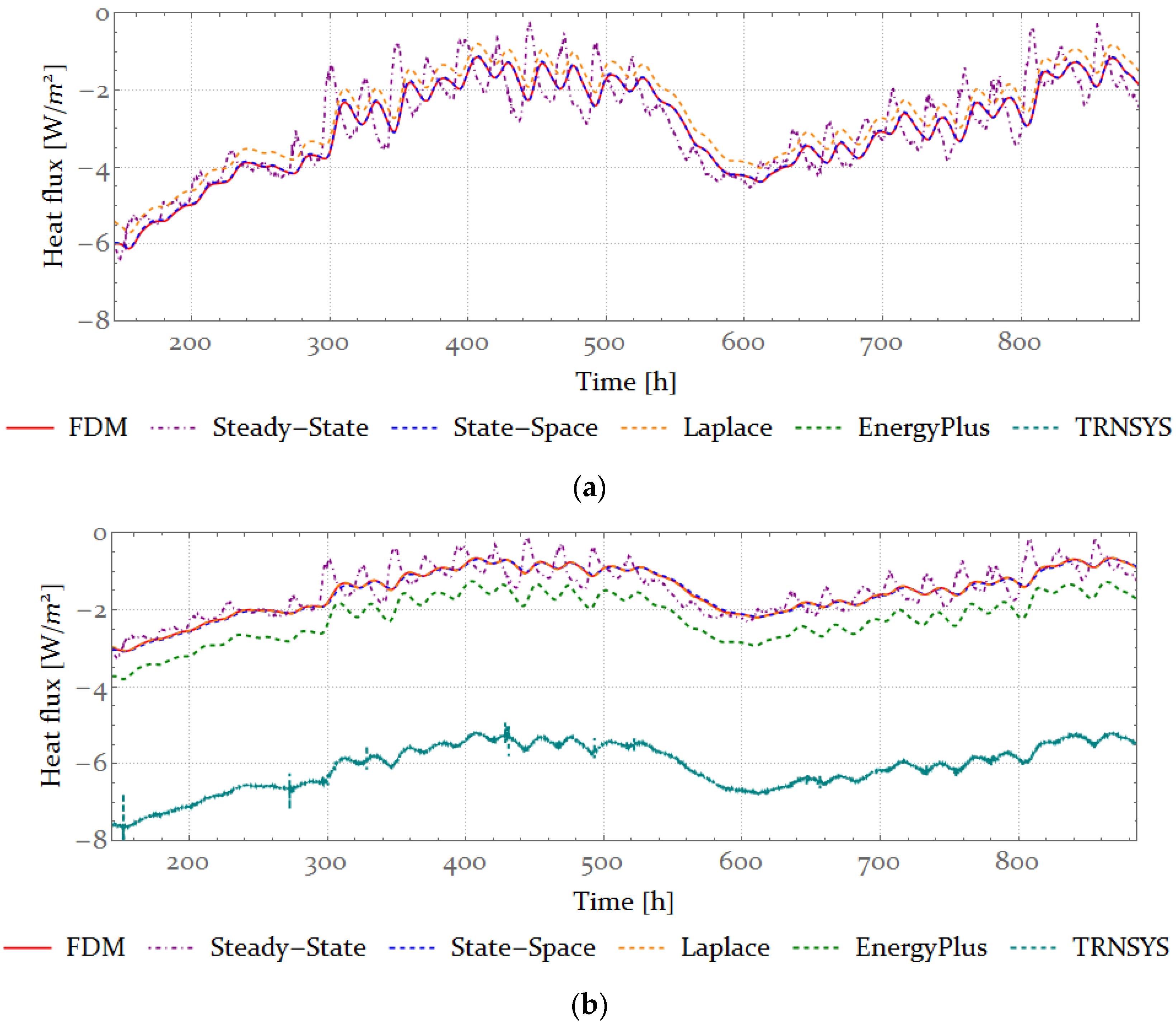
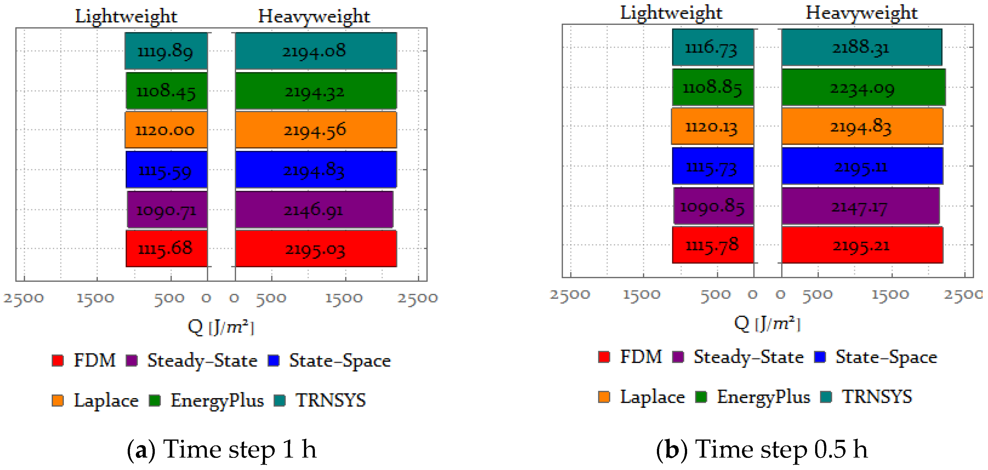
As a result of the analysis, the interior heat flux is calculated using Equations (6), (15), (19), (21) and (22) for time steps 1, 0.5, 0.25 and 0.1 h (
Figure 3,
Figure 4,
Figure 5 and
Figure 6). In addition, the total energy transferred through the interior surface of the element is calculated by integrating the heat flux function from t
min = 144 h to t
max = 864 h (
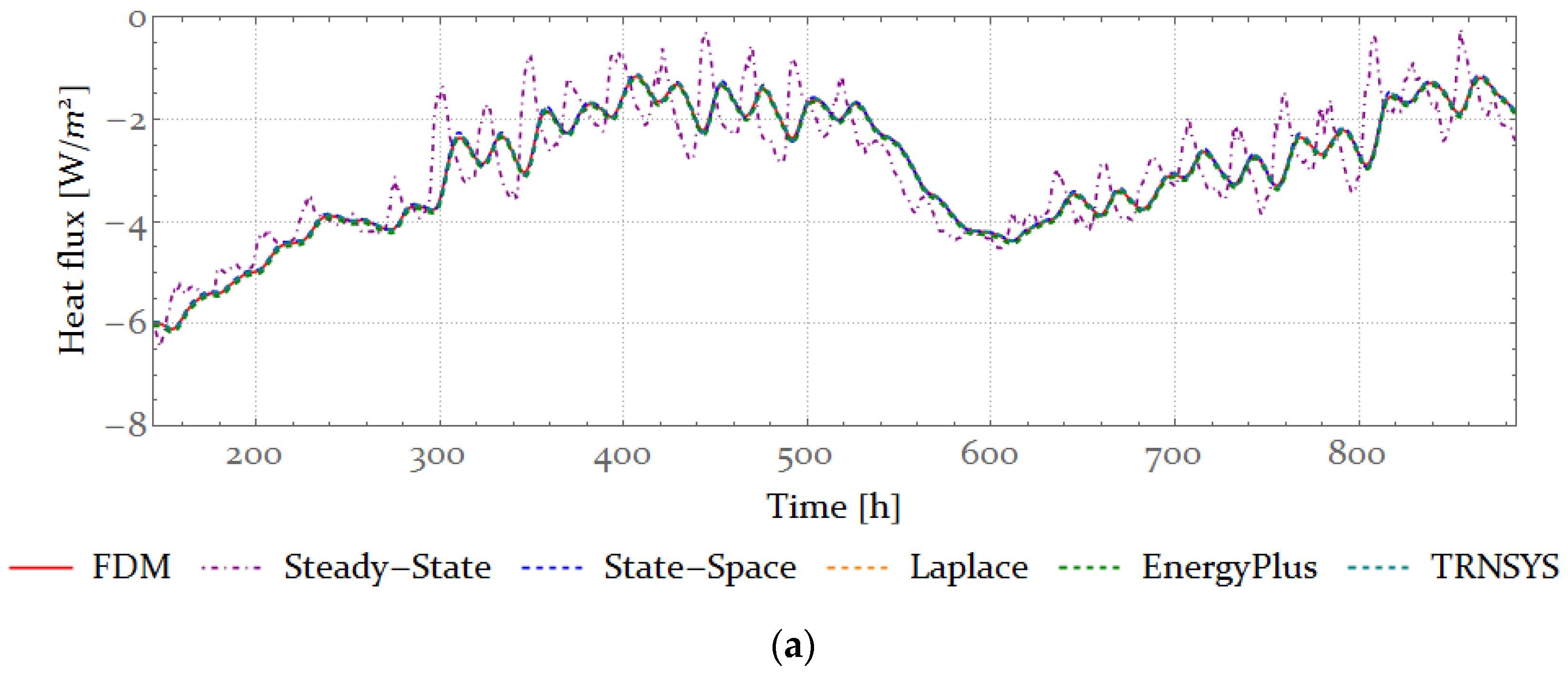
Figure 6b) the results for EnergyPlus and TRNSYS are not shown because they are numerically unstable, as can be seen in
Figure 7d.
Table 6 and
Figure 8 show the computational time required to calculate the interior heat flux function in the period from t
min to t
max for the FDM, the State-Space method and the Laplace method as implemented in Mathematica.
4. Comparison and Discussion
Two different types of wall elements were modelled—heavyweight and lightweight. For each wall element, the internal heat flux was calculated using six different procedures to show the effect of the wall’s thermal mass on the solution for different time steps used for the dynamic thermal simulation for all six procedures.
The solution of the FDM was taken as the reference point for the comparison. The number of subdivisions for the FDM solution was 100 with the step size of 0.390 cm for the heavyweight and 0.363 cm for the lightweight wall element. The solution of the FDM is calculated as described in
Section 2.1. The same subdivision used for the FDM was used for the State-Space method.
In
Table 4 and
Table 5, the stability of all procedures can be seen. For the heavyweight wall element, all methods show stable solutions for time steps of 1 h and 0.5 h (
Figure 3a and
Figure 4a). For time steps of 0.25 h and 0.1 h, the State-Space method and the Laplace method show stable solutions, while EnergyPlus and TRNSYS show a high deviation from the solution obtained with the FDM (
Figure 5a and
Figure 6a). For a time step of 0.25 h, this difference is as high as 31% for EnergyPlus and 78% for TRNSYS. In the case of a time step of 0.1 h, both EnergyPlus and TRNSYS give unreliable results. Although the algorithms of the State-Space method and the Laplace method implemented in the Mathematica for the purpose of this research are also implemented in EnergyPlus and TRNSYS, the heat flux calculated using EnergyPlus and TRNSYS is unstable for smaller time steps (
Figure 5a and
Figure 6a). This is due to the simplified procedures used for the calculation of matrix exponential in the case of the State-Space method implemented in EnergyPlus, and the root-finding algorithm for the Laplace method implemented in TRNSYS. In contrast, Mathematica uses a robust built-in algorithm for finding the matrix exponential and finding the roots of the denominator BB(s). In the case of the State-Space method, the number of subdivisions also affects the solution; however, not in terms of the stability of the CTF coefficients, but rather in terms of the overall accuracy of the calculated heat flux. As the number of subdivisions increases, the CTF coefficients for the State-Space method converge to a finite value.
For the lightweight wall element, all procedures show stable solutions for time steps of 1 h, 0.5 h and 0.25 h (
Figure 3b,
Figure 4b and
Figure 5b). For time steps of 0.1 h, the State-Space method and the Laplace method show stable solutions, while EnergyPlus and TRNSYS show a high deviation from the solution obtained with the FDM (
Figure 5b and
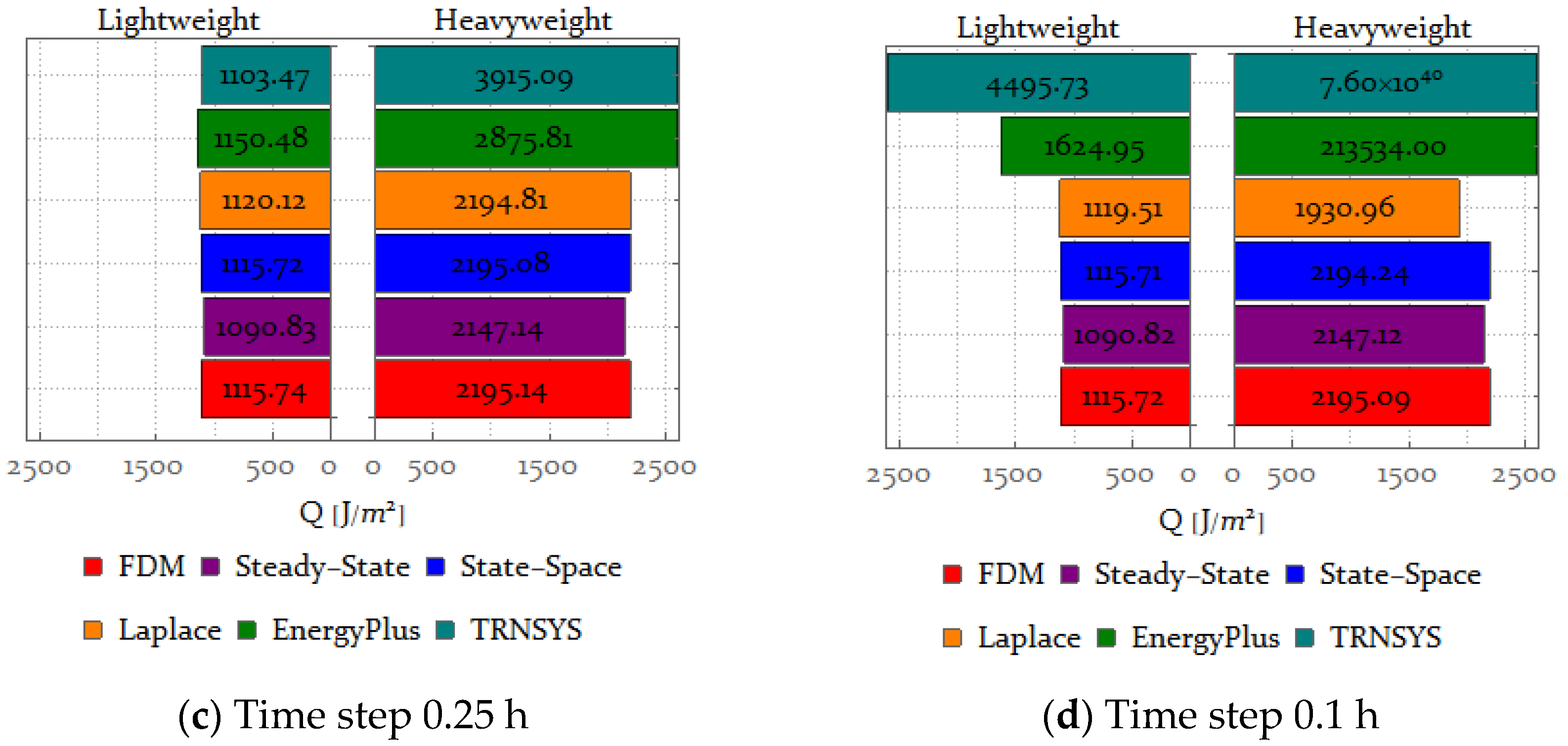
Figure 6b). For a time step of 0.1 h, the difference is 46% for EnergyPlus and 303% for TRNSYS.
The difference in total energy transferred through the interior surface can be seen in
Figure 7. For the lightweight wall element, the State-Space method and the Laplace method behave similarly for all time steps. There is no difference between the total energy transferred through the inner surface between the FDM and the State-Space method. For the Laplace method, this difference is negligible (0.39%). For the heavyweight wall element, the State-Space method is also stable for all time steps, and the difference between the total energy transmitted through the inner surface calculated using the FDM and the State-Space method is 0–0.04%. The Laplace method gives stable results for the time steps of 1 h, 0.5 h and 0.25 h, and the difference between the solution of the FDM and the Laplace method is 0.02%. For a time step of 0.1 h, the difference is 12.03%.
For the lightweight and heavyweight wall elements, EnergyPlus calculation produces more stable results than TRNSYS (
Figure 7). For the lightweight wall element, the difference between the total energy transferred through the inner surface between the FDM and EnergyPlus is 0.65–3.11% for time steps of 1 h, 0.5 h and 0.25 h, and for the time step of 1 h, that difference is 45.64%. On the other hand, the difference between FDM and TRNSYS is 0.04–0.31% for the 1 h and 0.5 h time steps, and 31.01% for the 0.25 h time step. For the 0.1 h time step, the results are unreliable as can be seen in
Figure 7d.
If the steady-state solution is considered, it can be seen that although the amplitude of the steady-state heat flux function is greater than that of the FDM, the difference between the total energy transferred through the inner surface between the FDM and the steady-state method is only 2.23% for the lightweight wall element and 2.19% for the heavyweight wall element (
Figure 3,
Figure 4,
Figure 5,
Figure 6 and
Figure 7). However, when the steady-state method is used to calculate the heat flux, the thermal mass of the element is not taken into account, which could lead to potential problems when designing mechanical systems and thermal comfort for the building’s occupants. This is especially important since one of the future directions of building energy management lies in the implementation of model predictive control (MPC).
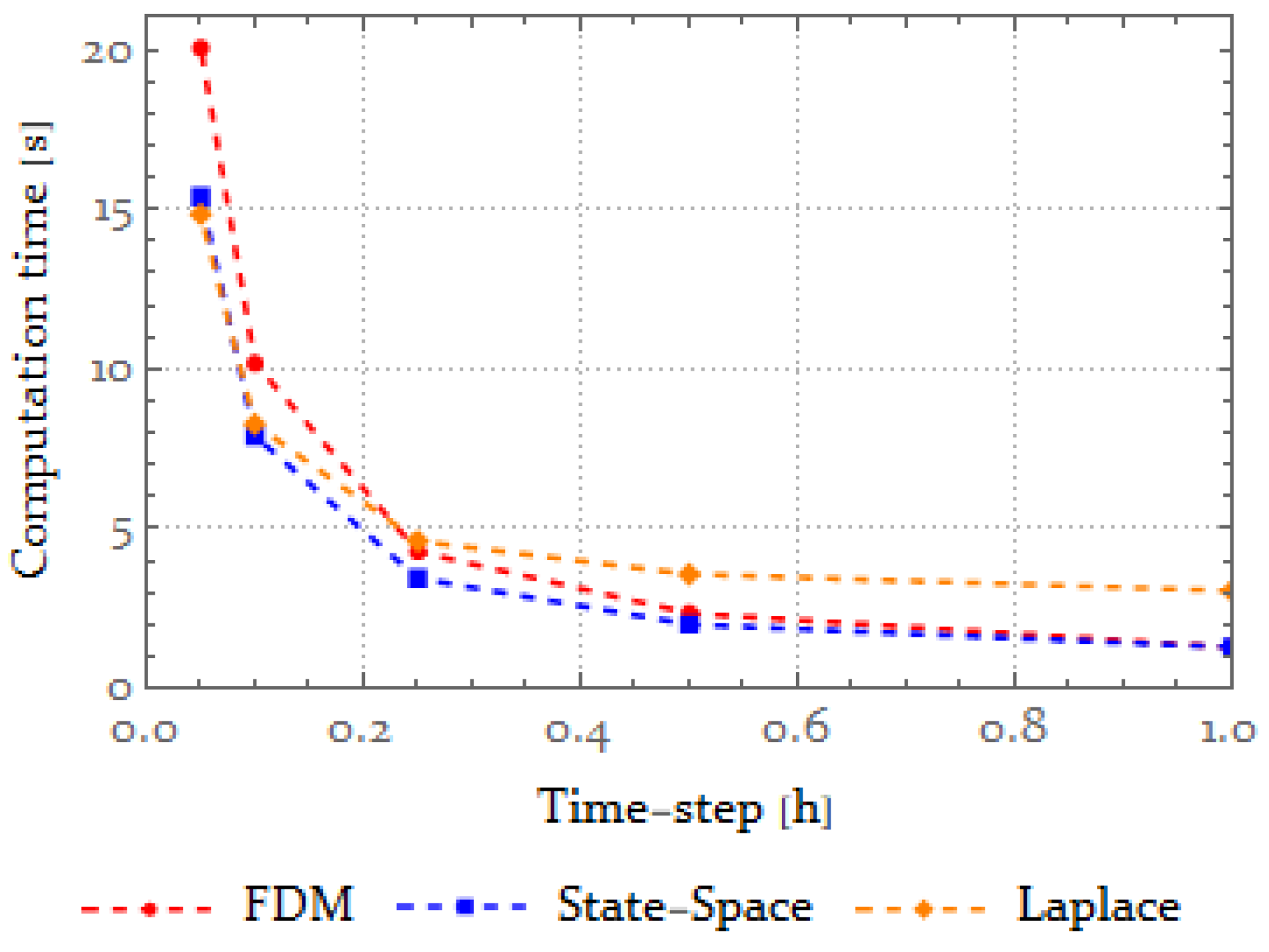
The computation times for the State-Space method, Laplace method and FDM are shown in
Figure 8 and
Table 6. For larger time steps, the State-Space method and the FDM perform similarly, while the Laplace method is much slower due to the interval for finding the roots of the denominator BB(s), which is 10
−8 for both the lightweight and heavyweight wall elements. For smaller time steps, the computation time for the State-Space method and the Laplace method is similar. In contrast, the computation time of the FDM becomes higher due to the number of linear systems that must be solved for each time step.
The State-Space method and the Laplace method implemented in the conventional software for dynamic energy simulations software could be improved by implementing more advanced algorithms for the calculation of the matrix exponential for the State-Space method and the root-finding procedure for the Laplace method, as these are the main drawbacks of the CTF methods. As is shown in the results, by using more advanced algorithms, both the State-Space method and the Laplace method were stable for smaller time steps in comparison to the results obtained from EnergyPlus and TRNSYS. This improvement for the calculation of the matrix exponential and the root-finding procedure comes at the cost of the computational time. However, if the goals set by the EU for the NZEBs and ZEBs are to be achieved, it is essential to improve the accuracy of the dynamic calculation for smaller time steps.
5. Conclusions
Dynamic methods are based on the non-stationary solution of the heat equation. This solution can be found numerically or analytically. Because of the long analysis period and the small time steps used for the analysis, numerical methods have proven to be insufficient for building energy simulations. Analytical methods such as conduction transfer functions (CTFs) have proven to be much better for building energy simulation problems and are implemented in modern dynamic energy simulation software such as TRNSYS and EnergyPlus. Among the most commonly used CTF methods are the Laplace method and the State-Space method. This research compares these two methods for the calculation of heat losses in heavyweight wall elements by implementing the algorithms from the research paper of Stephenson and Mitalas for the Laplace method and Seem for the State-Space method. These results are then compared with the results from TRNSYS and EnergyPlus.
TRNSYS uses the Laplace method to calculate the CTF coefficients and the bisection method to calculate the roots of the function BB(s), while EnergyPlus uses the State-Space method to calculate the CTF coefficients and the simplified methods such as the algorithm by Moler and Van Loan to calculate the matrix exponential. The goal of this paper is to show how well the Laplace method and the State-Space method perform for small time steps and heavyweight building elements and to show what opportunities exist to improve these methods by implementing more efficient algorithms for root-finding and the matrix exponential procedure. The finite difference method (FDM) is used as a reference point for the boundary heat flux density.
For the time steps of 1 h and 0.5 h, all methods (State-Space, Laplace, EnergyPlus and TRNSYS) were found to be adequate for both the heavyweight and lightweight wall elements. For the heavyweight wall element and a time step of 0.25 h, the difference between the total energy transferred through the inner surface was about 31% for EnergyPlus and 78% for TRNSYS compared to the solution obtained with the FDM. For the lightweight wall element, the results were stable for the time step of 0.25 h, but for the time step of 0.1 h, the difference between EnergyPlus and FDM was 45.64% while the difference between TRNSYS and FDM was 303%.
The State-Space method and the Laplace method implemented in Mathematica were stable for all time steps for both the heavyweight and lightweight wall elements due to the Mathematica’s powerful numerical and matrix manipulation algorithms. The maximum difference between the FDM and Mathematica was for the Laplace method and a time step of 0.1 h, where the difference was 12.03%. Therefore, one should choose the time step size accordingly, and avoid the smaller time steps if possible.
For the calculation of the total energy consumption, the steady-state method proved to be satisfactory. The difference between the FDM and the steady-state method was around 2.23% for the lightweight wall element and 2.19% for the heavyweight wall element.
The conclusions of this paper could be of interest for the implementation in NZEBs and ZEBs where thermal mass influences are relatively higher as well as for better power demand management strategies, which require accurate transient simulation of heavyweight and highly insulated building elements with short time steps (lower than or equal to 0.1 h, i.e., 6 min). On the other hand, the limitation of the research is that it involves a complex technique and requires high computational costs. This paper shows that the State-Space method and the Laplace method implemented in EnergyPlus and TRNSYS could be improved by implementing more advanced algorithms for the calculation of the matrix exponential for the State-Space method and the root-finding procedure for the Laplace method since these are the main drawbacks of the CTF methods. Further research will address the integration of more efficient algorithms with equal or smaller deviations from theoretical values.


