Abstract
Automated indoor environmental control is a research topic that is beginning to receive much attention in smart home automation. All machine learning models proposed to date for this purpose have relied on reinforcement learning using simple metrics of comfort as reward signals. Unfortunately, such indicators do not take into account individual preferences and other elements of human perception. This research explores an alternative (albeit closely related) paradigm called imitation learning. In the proposed architecture, machine learning models are trained with tabular data pertaining to environmental control activities of the real occupants of a residential unit. This eliminates the need for metrics that explicitly quantify human perception of comfort. Moreover, this article introduces the recently proposed deep attentive tabular neural network (TabNet) into smart home research by incorporating TabNet-based components within its overall framework. TabNet has consistently outperformed all other popular machine learning models in a variety of other application domains, including gradient boosting, which was previously considered ideal for learning from tabular data. The results obtained herein strongly suggest that TabNet is the best choice for smart home applications. Simulations conducted using the proposed architecture demonstrate its effectiveness in reproducing the activity patterns of the home unit’s actual occupants.
1. Introduction
The largest consumers of electricity in the US are residential units. In the year 2020, this sector alone accounted for approximately 40% of all electricity usage [1]. The average daily residential consumption of electricity is 12 kWh per person [2]. Therefore, effectively managing the usage of electricity in homes is vital to address global challenges around dwindling natural resources and climate change.
Recent advancements in sensor systems, automatic control, and machine learning, along with the proliferation of the IoT, have made smart homes practically feasible today [3,4,5]. A smart home allows energy to be utilized in an optimal manner, thereby reducing total resource consumption. This feat is accomplished in an automated fashion without the need for any direct human involvement. Various kinds of indoor appliances in a smart home can be controlled in this manner (cf. [6,7]), such as lighting, refrigeration, PHEV charging, battery storage, water pumps, and interior environmental control.
Environmental control in smart homes, primarily indoor temperature control, can be carried out while maintaining acceptable comfort levels for the home’s occupants. Conversely, comfort may be improved using automated scheduling without increasing energy consumption. A few recently published articles have aimed at making the second objective an attainable one.
An enabling tool of particular importance in this research direction is reinforcement learning. Reinforcement learning is an emerging machine learning paradigm that allows an algorithm to learn from experience (cf. [7]). In recent years, deep neural networks (DNNs) have emerged as the most popular machine learning models for a wide range of applications [8]. Consequently, research attention has been directed towards investigating deep reinforcement learning algorithms for smart home applications [9,10,11,12]. Deep reinforcement learning (DRL) algorithms that concentrate specifically on environmental control have begun to appear [13,14].
Recent research has proposed the use of reinforcement learning for indoor environmental control in smart homes. A significant amount of published research focuses on temperature regulation by controlling the HVAC system [15,16,17]. However, other published research focuses on controlling other equipment to manage the indoor temperature, such as the air conditioner alone [18], ventilation fan [19,20], underfloor heating [21], heat pumps [22], and the opening and closing of windows [23]. The main objective of such research is to minimize the energy cost while maintaining or increasing occupant [20]. However, only a few published articles focus on improving only occupant comfort [23,24]. It is worth mentioning that a substantial amount of such research considers indoor temperature as the only determinant of occupant comfort. Only a limited amount of research takes into consideration air quality (i.e., CO2 concentration) and/or visual comfort (i.e., lighting) [25].
In [22] the authors were able to reduce energy consumption by 4–11% while keeping the thermal comfort within an acceptable limit. Other research works have accomplished similar levels of reduction while maintaining temperature within a predefined threshold. Although the predicted mean vote (PMV) has not been used as a measure of comfort, it is assumed that comfort is directly determined by temperature. In [12], the proposed algorithm reduced the energy cost by 3.51% in winter and 4.05% in summer compared with the DDQN algorithm which achieving minimal comfort violation. In [24], comfort level was improved by about 15%; unfortunately, the associated energy cost increase was not addressed. In another article [23], the opening and closing of windows was controlled as a mean of improving thermal comfort and the air quality, without consuming electricity.
Elsewhere [25], the energy cost of a commercial building was reduced by more than 50% while maintaining comfort level by turning off the HVAC system and the lighting in the absence of any occupants. In another approach [26], a reinforcement learning agent exerted simultaneous control over the energy storage system and the HVAC system. The study reported a 17% increase in comfort and reduced power cost over a period of two months. A variant of a well known reinforcement learning approach (DDPG) was applied, with the RLlib library used to implement the learning agent and OpenAI Gym used for simulations. In [19], a reinforcement learning paradigm called double Q-learning was able to achieve a 10% reduction in the CO2 level and a 4–5% reduction in energy consumption while maintaining an acceptable PMV value. A total of 60 months of official climate data from Taipei were used to train the agent.
The present research explores avenues to automate environmental control by leveraging the latest advancements in machine learning. More specifically, it applies deep attentive tabular neural networks (TabNets) [27,28] for the twofold purposes of controlling the temperature settings within a smart home environment and predicting the temperature and humidity levels arising from it. It is the first among all known DNNs to outperform XGboost, the current best method to handle tabular data, for benchmark machine learning problems. Consequently, it is being investigated for a wide range of applications, such as the spread of COVID-19 [29], hyperspectral imagery [30], malware detection [31], and traffic prediction [32]. TabNet is based on the popular attention mechanism in deep learning cf. [33].
All of the studies mentioned above focused on using reinforcement learning as a method to replace human based control. In fact, this is a severe limitation, as the perception of comfort varies considerably from one person to another and is dependent on extraneous factors such as the occupants’ levels of physical activity and the time of day. In general, thermal comfort is nonlinear and not readily quantifiable. An earlier study [34] argued that thermal comfort measures are severely limited, as they do not consider human factors influencing comfort. In [35], the authors provided an overview of data collection and experimental research for assessing comfort levels under different climactic conditions. Various factors influencing thermal comfort and reviews of such comfort models are addressed in [36], along with a neural network-based model of comfort. The need to integrate human physiological and behavioral factors for accurate assessment of comfort is highlighted in [37], in which the authors put forward a workflow for personalized HVAC control. A recent study [38] evaluated thermal comfort models using computational fluid mechanics. Lastly, a number of reasons for integrating human health factors into comfort assessment methods are posited in [39].
In order to circumvent the reliance of reinforcement learning on the need to quantify the physical sensation of comfort, this research takes an alternate route, applying imitation learning, a paradigm that is strongly connected to reinforcement learning, in order to simulate human behavior while maintaining energy consumption at the same level. In treating humans as ‘experts’, it eliminates the need to quantify occupant comfort during the learning process (which is only used as an assessment tool in this article). Recent research has investigated adopting imitation learning for several tasks, ranging from dexterous robotics [40] to taxi driving [41]. Related energy applications include renewable energy sharing [42], smart grid load modeling [43], optimal scheduling [44], HVAC control [45], and distribution service restoration [46].
The research contributions of this study lie in the following directions:
- (i)
- To the best of the authors’ knowledge, this is the only smart grid-related research that uses TabNets, a DNN based model that currently outperforms all known machine learning algorithms for tabular data, including XGboost (extreme gradient boosting).
- (ii)
- The research proposes the use of imitation learning, a learning paradigm that has seldom if ever been investigated in the context of smart home environmental control.
- (iii)
- By applying imitation learning, the controlling agent is able to learn directly from recorded real human activity, thereby obviating the need for ad hoc quantification of occupant comfort.
- (iv)
- TabNet models are explored in this research for four separate tasks, i.e., predicting indoor temperature and humidity and controlling the switch settings of heating and cooling equipment.
In comparison with other machine learning models the results yielded by TabNet are very encouraging in terms of all four tasks assessed separately. Additionally, the proposed architecture consisting of four separate TabNet blocks is very effective in maintaining optimal comfort.
The remainder of this article is organized in the following manner. Section 2 provides the necessary background on those aspects of deep learning used in this research, including the layout of TabNet and an overview of imitation learning. Section 3 describes the overall architecture proposed in this article, consisting of four different TabNet blocks. Our simulation results are discussed in Section 4, and Section 5 concludes this article.
2. Background
A machine learning model receives inputs and produces outputs. Using a dataset of training samples, the model applies a learning algorithm to fine-tune its intrinsic parameters or weights, allowing it to acquire certain desirable performance characteristics. There are three broad classes of machine learning algorithms: (i) unsupervised learning, (ii) supervised learning, and (iii) reinforcement learning. In unsupervised learning, the model discovers hidden patterns in the dataset. For instance, it can learn to group inputs into clusters, or split signal sequences into statistically independent components. Supervised learning involves the presence of a supervisor. The learning model is trained to map inputs to their desired outputs (or targets). The model produces an output from each input training sample, while the supervisor provides the error, i.e., the difference between the model output and the desired value. Reinforcement learning is intermediate between the two classes; the supervisor is replaced by a critic, which provides reward feedback to the learning model that reflects the overall desirability of the latter’s output.
2.1. Deep Attentive Tabular Networks
TabNet consists of several functional DNN layers [28]. Before providing an overview of the layout of TabNet, an outline of each such layer is provided below.
A fully connected (FC) layer consists of a layer of neurons that incorporate a set of trainable weights along with sigmoid nonlinearities . Supposing that the vector input to an FC is denoted as , its corresponding output is provided by the following relationship:
Here, the mapping represents an elementwise application of ; thus, if is a scalar input, the output is provided by
It must be noted that in this article symbols for scalar quantities appear in italics, whereas those for vectors appear in bold.
TabNet contains layers of generalized linear units (GLUs). With representing the input to a GLU layer, the output is
The operator ‘’ in the above relationship is the Hadamard product. The main advantage of using GLU layers in TabNet is to allow penetration into deeper layers without encountering exploding or imploding gradients.
Another type of layer consists of rectified linear units (ReLu). If is the input vector to such a layer, its corresponding output is denoted as , where is the elementwise application of the function:
Training samples in TabNet are divided into minibatches. A batch normalization (BN) layer contains neurons with linear activations, their only purpose being to perform elementwise normalization of their inputs. If is a minibatch and the vectors and denote the input and output of any BN layer, then , where represents elementwise batch normalization.
For each element of ,
The maximization and minimization operations are carried out over all sample elements in minibatch . In this manner each element of the vector is restricted to lie within the unit interval [0, 1].
Throughout the remainder of this article, is used to represent a vector input to TabNet such that , where is the input dimensionality. Although in general its output is a vector, the TabNet architecture used in this research outputs a scalar . Optionally, the th sample input and output are indicated as and . TabNet is designed to mimic decision trees. It follows a multi-step architecture in which each sequential step is analogous to a decision box in a decision tree. Figure 1 illustrates the arrangement of a step indexed in TabNet. Each step includes two transformer blocks, (i) an attentive transformer and (ii) a feature transformer, with their layouts depicted in Figure 2 and Figure 3, respectively.
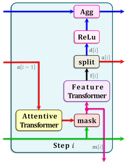
Figure 1.
TabNet Step. A single step, indexed , in the overall multi-step TabNet layout. The pathways for each signal follow a different color.
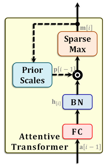
Figure 2.
Attentive Transformer. The layout of the attentive transformer used in TabNet. The black circle marked ‘’ represents elementwise multiplication, while the dashed lines are paths leading from the previous time step .
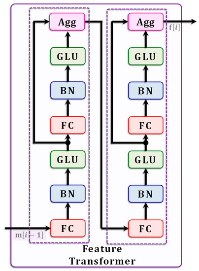
Figure 3.
Feature Transformer. The layout of the feature transformer used in TabNet. It consists of four subunits, with each containing an FC, BN, and GLU; two of the subunits have Agg blocks as well.
The attentive transformer at each step incorporates a SparseMax block that implements a sparse version of the well-known softmax function [47]. It produces a sparse vector , labeled as the block mask. The mask is a sparse vector of probabilities that can be obtained in the following manner:
In the above equation, is a subspace of probability simplices in dimensions with only nonzero elements. In other words, the mask vector in Equation (6) is such that and . The vector in Equation (6) appearing above is obtained as follows:
Ignoring the BN block, here the function is a trainable mapping accomplished by the immediately preceding FC layer, as in Equation (1). The FC layer has its own set of trainable weights, although for simplicity is has not been shown in the figure.
The block priorScales used in the attentive transformer in step (Figure 1) is a vector . It is used to scale down using the masks from all prior steps . With being a predetermined TabNet parameter vector, the mask is obtained as shown below:
The product in the above equation is carried out in an elementwise fashion. The rationale behind this formulation can be explained in the following manner. If a scalar element has been used extensively in some prior step , the corresponding mask will be close to one. The corresponding factor in Equation (8) will be small, meaning that the same element is scaled downward. On the other hand, if the element stays relatively unused, then will be nearly equal to one, ergo likelier to be used in step .
The feature transform converts input vectors into more suitable representations. It consists of four separate sub-blocks, with each sub-block consisting of an FC layer followed by a BN layer and then a GLU layer. The transformer applies normalization in the manner shown in Equation (5); however, it uses ghost normalization, where only a smaller set of the minibatch is used for this purpose, meaning that . Although this slows down the training process, ghost normalization has been shown to yield better generalization properties [48].
The feature transformer splits the vector into two disjoint chunks with dimensionalities and such that . This is achieved using the Split block. Aggregation takes place at each block Agg. The final decision is determined as follows:
The mapping appearing above is performed elementwise, as in Equation (4). The quantity is the total number of steps in TabNet, which is obtained empirically based on the dataset. The overall layout of TabNet is shown in Figure 4 (in the figure, the term ‘step’ does not refer to algorithmic iterations; these steps are akin to physical blocks, with the terminology used in this article being borrowed from [28]).
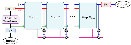
Figure 4.
TabNet Layout. The overall multi-step layout of TabNet. The colors of the signal pathways follow the same convention as in Figure 1.
With the symbol representing the vector of all weight parameters of TabNet and being another nonlinearity representing the composition of the functions of each step, TabNet’s output can be expressed succinctly as
The training dataset is of the form , where is the set of indices of all training samples, is the th sample input, and is the corresponding target output. The aim of the learning algorithm is to iteratively increment such that for every training sample the difference between the target and TabNet’s true output is steadily reduced. The deviation between the outputs and the targets is quantified in terms of the network’s loss. A regularization term is added to the loss, and the regularized loss is denoted as , whereupon the TabNet trained parameter is
For the purpose of training, the training samples in are divided into mutually disjoint minibatches. Supposing that is a minibatch and is the algorithm’s learning rate, each increment is applied iteratively in accordance with the rule shown below:
In each epoch of the training algorithm, the parameter vector is incremented separately for every minibatch, meaning that the end of that epoch roughly marks a single gradient step with loss . As long as is sufficiently small, the loss continues to decrease with each epoch. At the end of the epoch, is shuffled randomly and split into minibatches for the next epoch.
The training algorithm is allowed to proceed for several such epochs. The termination criterion is determined with the help of another dataset , called the validation dataset; note that . The algorithm is terminated when the loss begins to rise. At this stage, is treated as the estimate of the network’s optimal parameter . Here, represents the entire space of all real-world data, with . As long as the datasets and are sampled randomly from using the latter’s underlying probability distribution, it can be shown that is the most likely estimate of the true optimum. Thereafter, TabNet can be deployed for its intended real-world application.
2.2. Imitation Learning
In reinforcement learning terminology, an agent is a learning entity that exerts control over a stochastic external environment by means of a sequence of actions over time [7]. The agent learns to improve the performance of its environment using reward signals that are derived from the latter. Rewards are quantitative metrics that indicate the immediate performance of the environment (e.g., the occupant ‘s instantaneous comfort) [49,50]. The sets and are the state and action spaces, and may be either discrete or continuous. Signals are sampled at discrete regularly spaced time instants , where and is the time horizon. The current state of the environment is available to the agent through a vector of features, such as sensor measurements, which then implements an action . The environment transitions to the next state and returns an immediate reward signal , with denoting the environment’s reward function, which is unknown to the agent. The transition can be denoted concisely as Actions taken by the agent are determined in accordance with a policy , which is a probability distribution over actions in such that .
The value of any state under a policy is the expected sum of rewards when the environment is initialized to that state, i.e., . Current deep reinforcement learning methods typically make use of samples that are stored in the replay buffer . These samples are of the form , where actions are carried out under policies designed to explore the unknown environment. The learning algorithm proceeds by drawing samples randomly from the buffer in minibatches. It aims to infer the optimal policy . Such a policy, which is not known a priori, is the one under which the values of every state in are at the maximum. Mathematically, the optimal policy is defined as
Imitation learning aims to accomplish the reverse of reinforcement learning. The buffer contains samples that are obtained externally from an expert and without the agent’s involvement. Such an expert may represent an actual human being or multiple humans. It may be assumed that the expert applies the optimal policy . In such a case, the samples in the buffer are of the form , with actions . The differences between reinforcement learning and imitation learning are highlighted in Figure 5.
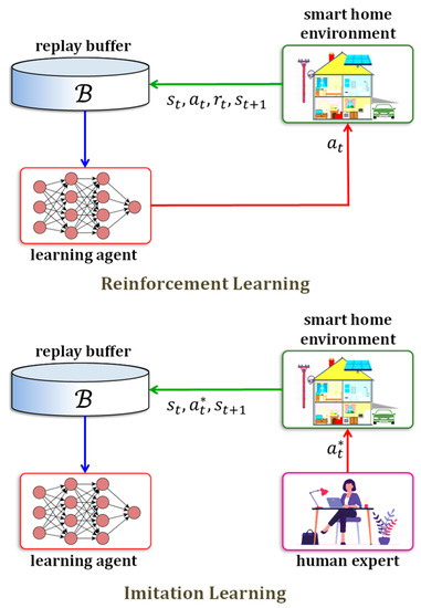
Figure 5.
Reinforcement Learning vs. Imitation Learning. Illustration highlighting the difference between the reinforcement learning and imitation learning paradigms. Signal flow pathways in reinforcement learning (top) and in imitation learning (bottom). In reinforcement learning for indoor environmental control, the reward signal is based directly on comfort indices that may not be suitable. Imitation learning does not use , as the action is replaced with the optimal action . This is possible because imitation learning makes explicit use of an expert, i.e., the home’s actual resident(s), whose prior history of actions reflect the true comfort level.
A recent article [7] has provided a comprehensive exposition of reinforcement learning as well as an in-depth survey of its various smart home applications.
3. Proposed Approach
3.1. Policy Models
As the dataset contains separate heating and cooling controls, two policy models are used in this research to represent agents for imitation learning. The models share a common input :
The models are represented in functional form with the parameters (heating) and (cooling); the common subscript is used to distinguish them from the prediction models. This choice is motivated by the observations that in the reinforcement learning literature is often used to represent model parameters, such a neural network weights, while is used to denote policies. The function for the heating model is provided below:
Similarly, the corresponding function for the cooling model is
It must be noted that the quantities and (with the ‘hat’ ) are merely the settings that are recommended by the agent model.
Because the thermostat settings do not change in each time step, adjusting them at any instant to their recommended values is implemented in a probabilistic manner. Therefore, with the probability of switching to the recommended setting being , the heating setting at time instant is obtained as follows:
Similarly, the cooling setting at the same instant is
The symbols and (with the ‘hat’ ) in the above expressions are used to distinguish them from manually controlled settings available in the dataset. The schematic in Figure 6 shows the proposed architecture. The schematic shows a switch to regulate the vector , which is probabilistically determined based on the probability parameter . Suppose that at a 15 min time interval the setting is . During this period, the control model proposes a new setting , which is its action. At the beginning of the next instant , the setting vector is adjusted with a probability in accordance with the control action such that . Otherwise, no change is made to the setting, which remains the same as in the previous instant, whence .
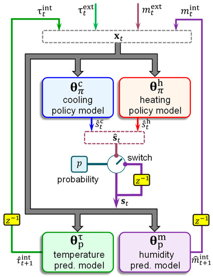
Figure 6.
Proposed Architecture. Schematic showing the architecture proposed in this research for indoor environmental control. The small boxes labeled represent time delays. The architecture includes four TabNets and a probabilistic switch. The layout depicts how the proposed architecture is configured during real-time usage. Each TabNet is trained separately with appropriate samples.
3.2. Prediction Models
The purpose of the environmental prediction models is to predict the future indoor temperature and humidity levels. This is because when the policy models and are used to replace human decisions, the actual recorded indoor temperature and humidity levels from the dataset can no longer be used. Because only single-step lookahead predictions are required, two prediction models have been used with a common subscript for prediction, namely, (temperature) and (humidity). In addition to in Equation (14), the inputs to these models are the vectors of the switching actions, obtained using Equations (17) and (18), as shown below:
The predictions of the TabNet models can be expressed in functional form. The form corresponding to temperature prediction is shown below:
The analogous expression for predicting humidity is
3.3. Comfort Indices
Human comfort level is determined by a combination of several factors, including the indoor temperature and humidity. As noted earlier, comfort is a human sensation that varies from one individual to another. Moreover, as it incorporates nonlinearities, linear quantification of comfort may not reflect the true occupant comfort. Consequently, quantified comfort metrics are not used anywhere in this article to train the TabNet models, and are only used as a secondary evaluation tool. The two indices used here for secondary evaluation are (i) the predicted mean vote (PMV) and (ii) the predicted percentage of dissatisfied (PPD). Although PMV and PPD [49,50] are both numerical indices reflecting dissatisfaction, they are nonetheless referred to as ‘comfort’ indices.
PMV estimates the mean response of a large group of people in accordance with the ASHRAE thermal sensation scale. The index is an integer in the interval , with zero representing the highest satisfaction. The PMV at any time instant can be obtained in accordance with the following expression:
In Equation (22), , and are three constants with appropriate units; their respective numerical values are provided in Table 1. It should be noted that these values, which are obtained from [50], are different for males, females, and mixed-gender occupants. Secondary determinants of human comfort, such as clothing, etc., could not be incorporated into Equation (22), as they were not available in the dataset.

Table 1.
Numerical values of PMV and PPD constants.
The PPD index estimates the percentage of a group of people who report dissatisfaction, with zero reflecting maximum comfort. It can be obtained from PMV [50] in a straightforward manner, as shown below:
The numerical values of the three constants , , and in Equation (23) are supplied in Table 1.
3.4. Evaluation Metrics
The accuracy of a model was determined as the sum of the adjusted absolute differences between real values and the corresponding TabNet output values:
In the above Equation (22), is the total number of samples (i.e., or , as the case may be), and is a Kronecker delta function defined as follows:
In Equation (25), is the error tolerance, is the TabNet output at time instant , and is the corresponding true value. The symbol denotes any one of , , , and . The values assigned to the error tolerance were for the prediction models and for the policy models. This error margin was incorporated to circumvent the degree of inherent randomness when the settings are under human control. Thus, a difference of less than 5% between the model’s recommended heater setting and the real human adjustment in the dataset was not considered to be inaccurate. Although in Equation (24) was primarily adopted to assess the performance of the policy models , it was used as a secondary performance metric for the prediction models as well, albeit with a lower tolerance.
The mean square error between and its predicted value is
As before, in Equation (26) above The primary purpose of this metric is to gauge the performance of the prediction models . Furthermore, the error is used in conjunction with the policy models as an additional metric for performance evaluation.
4. Results
4.1. Data Preprocessing
The dataset used in this research takes the form of time series samples. The time series contains outside (external) and indoor (internal) temperatures and , corresponding humidity levels and , and separate thermostat settings for heating and cooling and . The subscripts appearing in all these quantities refer to discrete time instances with , where is the length of a sample training. The temperatures are specified in °F (degrees Farhenheit) and the humidity levels as percentages, with 0% and 100% representing no water content and full saturation, respectively. The initial dataset included various other fields that were not required in this research.
Two separate settings ( and ) are used here only because that was the case in the dataset. We hypothesize that this is a residence-specific artifact. Depending on the scenario, a single thermostat setting variable may be used, leading to a simpler architecture with only a single policy model.
The samples in the dataset were collected at regularly spaced intervals of 15 min, meaning that the lapsed time between any two consecutive instants and was 15 min. Although time instances over whole days of 24 h were available for multiple months, only time intervals from 6:00 a.m.–8:00 a.m. and from 6:00 p.m.–8:00 p.m. during workdays were used, as these were the intervals during which the data consistently showed that the settings were adjusted often, indicating the presence of occupants. Accordingly, the time length was . Weekends and holidays were discarded, as there was no consistent pattern of activity. Samples during the months of September and October were selected, as it was during these periods that the temperature settings were most frequently adjusted in both increasing and decreasing directions.
The two-hour periods were then divided into two categories, (i) active and (ii) inactive. Periods during which any switching activity could be observed were regarded as active periods, while those with no such activity were treated as inactive periods. Table 2 shows the total number of samples present in each category and the percentage of times the thermostat settings for heating and cooling were adjusted.
Table 2.
Samples in dataset.
4.2. Training
To train the policy models (), the same set of four fields, , , and , i.e., the inside and outside temperatures and humidity levels, were treated as inputs. The heater setting and the cooler setting were the targets (i.e., desired outputs) for and . Only samples from the active periods were used during model training. Of these samples, 80% was used explicitly for training, yielding a total of 4269 samples in for and 1258 such samples for . The remaining 20% of samples was set aside in order to evaluate the policy models’ performances in . Figure 7 show the steady reduction in the mean square errors with increasing iterations for both policy models.
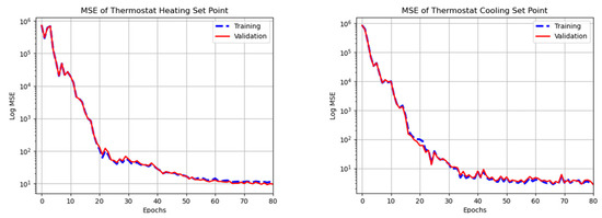
Figure 7.
Policy Model Training. Plots showing logarithms of mean squared errors with respect to training samples (dashed blue) and validation samples (solid red) as a function of training iteration for (left) and (right).
In order to train the prediction models (), four fields from the dataset, namely, , , , and , made up one set of inputs, while the temperature and humidity level made up the other. Because the purpose of these models was to predict the internal temperature and humidity after a single time step of 15 min, the values and were the targets (i.e., desired outputs), corresponding to the temperature and humidity prediction models, and . The samples were divided into training and validation sets consisting of 80% and 20% of the total, respectively. The steady convergence of the mean square error as training progressed is shown in Figure 8.
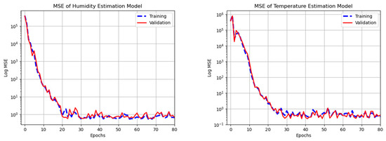
Figure 8.
Prediction Model Training. Plots showing logarithms of the mean squared error with respect to training samples (dashed blue) and validation samples (solid red) as a function of training iterations for (left) and (right).
4.3. Model Comparison
The four TabNet components of the proposed model shown earlier in Figure 6 were evaluated in terms of their accuracy and mean squared error . Simulations were carried out to compare the performance levels of the proposed TabNet models with seven of the most commonly used machine learning algorithms for regression: (i) deep neural network, (ii) K-nearest neighbors, (iii) decision tree, (iv) random forest, (v) adaBoost, (vi) gradient boosting, and (vii) support vector regression. Pytorch implementations of these regression models are available online [51]. As each component of the proposed architecture was separately investigated, these are referred to as open loop simulations.
The performances of the policy models and as per Equations (23) and (25) are provided in Table 3, while those of the prediction models and are shown in Table 4. The accuracy and the mean squared error obtained from TabNet and the other learning models listed above are shown in both tables. The best performance in each of the eight cases (four models × two measures) is highlighted in bold.
Table 3.
Performances of policy models.
Table 4.
Performances of prediction models.
It can be seen that TabNet outperforms all other models for all four tasks and in terms of both the and metrics. In addition, it can be observed that gradient boosting performs better in both policy models than the other six models used for comparison. This observation is not surprising, as gradient boosting [52] was considered the model of choice for dealing with tabular data before TabNet was proposed.
Having clearly established the efficacy of the TabNet components in the proposed architecture, the purpose of the next study was to test the efficacy of the overall architecture. Closed loop simulations were conducted where the proposed architecture was implemented in its entirety, as depicted in Figure 6. All four TabNet components were allowed to operate in tandem. Under these circumstances, the heating and cooling settings were controlled by the policy TabNets and , and the values available in the dataset could no longer be used. Ergo, the inputs to and were determined in accordance with Equations (15)–(18).
4.4. Comfort
The PMV indices were obtained for female, male, and mixed-gender occupants for various values of the switching probability , as shown in Figure 9. A steady improvement in the comfort (i.e., drop in PMV) can be seen as is increased from to in increments of . The maximum comfort level is attained when the settings are adjusted every 15 min, i.e., when . Figure 10 shows the analogous PPV indices. Due to its direct relationship with PMV, the plots in Figure 10 look very similar to those in Figure 9.
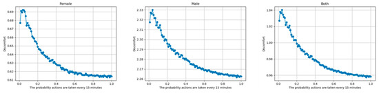
Figure 9.
PMV vs. Probability. PMV with increasing switching probability for females (left), males (middle), and mixed-gender groups (right).
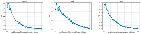
Figure 10.
PPV vs. Probability. PPV with increasing switching probability for females (left), males (middle), and mixed-gender groups (right).
Furthermore, it can be observed that both indices have the lowest values when PMV was calculated for female occupant(s), followed by mixed gender occupants, and are highest for male occupant(s). This relationship was met regardless of the switching probability. Moreover, it can be seen that the gender-based differences are numerically very significant. This observation strongly indicates that the source of the dataset was from a home unit with one or more female occupants, and that training the proposed TabNet-based architecture on such data resulted in its fine-tuning to maximize female comfort.
5. Conclusions
Two major inferences can be drawn from this research. First, the results obtained from the open loop simulations conclusively establish the effectiveness of TabNet for handling smart home environment-related tabular data for prediction and control tasks. Despite their superior performance with other types of data, conventional deep neural networks have not been able to outperform gradient boosting for tabular data [27,28]. This study corroborates nearly identical research findings that have been reported within the past year, all of which indicate that TabNet is better equipped than gradient boosting for similarly structured data in other applications. Gradient boosting has been used in similar applications to lower energy costs [53]. This investigation, as well as other similar efforts in smart home environment control, stand to benefit directly from the findings of the present research.
Second, this study illustrates that the proposed TabNet-based architecture can be trained using imitation learning to automate environmental control in home interiors. In contrast to reinforcement learning [7], the proposed approach obviates the need to use generic comfort indices. PMV and PPD [50], which are drawn using binary votes of large mixed-gender groups of individuals, are useful in designing ventilation, air conditioning, and other systems in buildings and homes as well as in establishing construction standards for large scale use; however, they are not meant to measure a specific individuals’ perceptions of comfort. Proper quantification of the actual comfort sensation felt by either individual occupants or families living in home units requires individual real-time monitoring of the occupants’ instantaneous physiological responses [54,55]. Because such invasive procedures are impractical for daily use, imitation learning more suitable for smart home automation than reinforcement learning [7].
In the absence of any direct information on the pricing policy or estimates of what the indoor temperature would be without any heating or cooling at each instant, it is impossible to determine how the probability of a given setting change affects energy consumption. However, it can safely be assumed that a real home occupant would not change the settings every 15 min even if she/he wanted to. Adjusting the probability parameter using the proposed method helps to maximize comfort while avoiding adversely effects on energy consumption costs.
During actual installation in any smart home, the TabNet models in the proposed architecture can be personalized using pre-recorded histories of manual temperature setting adjustments specific to the unit. Alternatively, pretrained models can be fine-tuned online for the occupants’ individualized comfort using real-time data streams of the occupants’ activity patterns. Such training can be achieved in a manner similar to that proposed for XGboost in [56].
Author Contributions
Conceptualization, S.D.; Methodology, O.a.-A. and S.D.; Software, O.a.-A.; Validation, O.a.-A.; Formal analysis, S.D.; Investigation, S.D.; Data curation, H.W.; Writing—original draft, S.D.; Visualization, O.a.-A.; Supervision, S.D. All authors have read and agreed to the published version of the manuscript.
Funding
This research received no external funding.
Data Availability Statement
The data used in this research was obtained from [57].
Conflicts of Interest
The authors declare no conflict of interest.
References
- U.S. Energy Information Administration. Electricity Explained: Use of Electricity. 14 May 2021. Available online: https://www.eia.gov/energyexplained/electricity/use-of-electricity.php (accessed on 10 April 2022).
- Center for Sustainable Systems. U.S. Energy System Factsheet; Pub. No. CSS03-11; Center for Sustainable Systems, University of Michigan: Ann Arbor, MI, USA, 2021; Available online: https://css.umich.edu/factsheets/us-energy-system-factsheet (accessed on 10 April 2022).
- Shareef, H.; Ahmed, M.S.; Mohamed, A.; Al Hassan, E. Review on Home Energy Management System Considering Demand Responses, Smart Technologies, and Intelligent Controllers. IEEE Access 2018, 6, 24498–24509. [Google Scholar] [CrossRef]
- Marikyan, D.; Papagiannidis, S.; Alamanos, E. A systematic review of the smart home literature: A user perspective. Technol. Forecast. Soc. Chang. 2019, 138, 139–154. [Google Scholar] [CrossRef]
- Li, W.; Yigitcanlar, T.; Erol, I.; Liu, A. Motivations, barriers and risks of smart home adoption: From systematic literature review to conceptual framework. Energy Res. Soc. Sci. 2021, 80, 102211. [Google Scholar] [CrossRef]
- Ali, H.O.; Ouassaid, M.; Maaroufi, M. Chapter 24—Optimal appliance management system with renewable energy integration for smart homes. In Renewable Energy Systems; Academic Press: Cambridge, MA, USA, 2021; pp. 533–552. ISBN 9780128200049. [Google Scholar] [CrossRef]
- Al-Ani, O.; Das, S. Reinforcement Learning: Theory and Applications in HEMS. Energies 2022, 15, 6392. [Google Scholar] [CrossRef]
- Goodfellow, I.; Bengio, Y.; Courville, A. Deep Learning; MIT Press: Cambridge, MA, USA, 2016; Available online: http://www.deeplearningbook.org (accessed on 2 February 2022).
- Yu, L.; Qin, S.; Zhang, M.; Shen, C.; Jiang, T.; Guan, X. Deep reinforcement learning for smart building energy management: A survey. arXiv 2020, arXiv:2008.05074. [Google Scholar]
- Yu, L.; Xie, W.; Xie, D.; Zou, Y.; Zhang, D.; Sun, Z.; Zhang, L.; Zhang, Y.; Jiang, T. Deep Reinforcement Learning for Smart Home Energy Management. IEEE Internet Things J. 2020, 7, 2751–2762. [Google Scholar] [CrossRef]
- Lissa, P.; Deane, C.; Schukat, M.; Seri, F.; Keane, M.; Barrett, E. Deep reinforcement learning for home energy management system control. Energy AI 2021, 3, 100043. [Google Scholar] [CrossRef]
- Yang, T.; Zhao, L.; Li, W.; Wu, J.; Zomaya, A.Y. Towards healthy and cost-effective indoor environment management in smart homes: A deep reinforcement learning approach. Appl. Energy 2021, 300, 117335. [Google Scholar] [CrossRef]
- Gupta, A.; Badr, Y.; Negahban, A.; Qiu, R.G. Energy-efficient heating control for smart buildings with deep reinforcement learning. J. Build. Eng. 2021, 34, 101739. [Google Scholar] [CrossRef]
- Svetozarevic, B.; Baumann, C.; Muntwiler, S.; Di Natale, L.; Zeilinger, M.N.; Heer, P. Data-driven control of room temperature and bidirectional EV charging using deep reinforcement learning: Simulations and experiments. Appl. Energy 2022, 307, 118127. [Google Scholar] [CrossRef]
- Lu, S.; Wang, W.; Lin, C.; Hameen, E.C. Data-driven simulation of a thermal comfort-based temperature set-point control with ASHRAE RP884. Build. Environ. 2019, 156, 137–146. [Google Scholar] [CrossRef]
- Macieira, P.; Gomes, L.; Vale, Z. Energy Management Model for HVAC Control Supported by Reinforcement Learning. Energies 2021, 14, 8210. [Google Scholar] [CrossRef]
- Liu, B.; Akcakaya, M.; Mcdermott, T.E. Automated Control of Transactive HVACs in Energy Distribution Systems. IEEE Trans. Smart Grid 2021, 12, 2462–2471. [Google Scholar] [CrossRef]
- Zhang, X.; Biagioni, D.; Cai, M.; Graf, P.; Rahman, S. An Edge-Cloud Integrated Solution for Buildings Demand Response Using Reinforcement Learning. IEEE Trans. Smart Grid 2021, 12, 420–431. [Google Scholar] [CrossRef]
- Valladares, W.; Galindo, M.; Gutiérrez, J.; Wu, W.-C.; Liao, K.-K.; Liao, J.-C.; Lu, K.-C.; Wang, C.-C. Energy optimization associated with thermal comfort and indoor air control via a deep reinforcement learning algorithm. Build. Environ. 2019, 155, 105–117. [Google Scholar] [CrossRef]
- Zhang, Z.; Ma, C.; Zhu, R. Thermal and Energy Management Based on Bimodal Airflow-Temperature Sensing and Reinforcement Learning. Energies 2018, 11, 2575. [Google Scholar] [CrossRef]
- Blad, C.; Bøgh, S.; Kallesøe, C. A Multi-Agent Reinforcement Learning Approach to Price and Comfort Optimization in HVAC-Systems. Energies 2021, 14, 7491. [Google Scholar] [CrossRef]
- Ruelens, F.; Iacovella, S.; Claessens, B.; Belmans, R. Learning Agent for a Heat-Pump Thermostat with a Set-Back Strategy Using Model-Free Reinforcement Learning. Energies 2015, 8, 8300–8318. [Google Scholar] [CrossRef]
- Han, M.; May, R.; Zhang, X.; Wang, X.; Pan, S.; Da, Y.; Jin, Y. A novel reinforcement learning method for improving occupant comfort via window opening and closing. Sustain. Cities Soc. 2020, 61, 102247. [Google Scholar] [CrossRef]
- Dmitrewski, A.; Molina-Solana, M.; Arcucci, R. CntrlDA: A building energy management control system with real-time adjustments. Application to indoor temperature. Build. Environ. 2022, 215, 108938. [Google Scholar] [CrossRef]
- Korkidis, P.; Dounis, A.; Kofinas, P. Computational Intelligence Technologies for Occupancy Estimation and Comfort Control in Buildings. Energies 2021, 14, 4971. [Google Scholar] [CrossRef]
- Kodama, N.; Harada, T.; Miyazaki, K. Home Energy Management Algorithm Based on Deep Reinforcement Learning Using Multistep Prediction. IEEE Access 2021, 9, 153108–153115. [Google Scholar] [CrossRef]
- Arik, S.O.; Pfister, T. TabNet: Attentive interpretable tabular learning. arXiv 2020, arXiv:1908.07442v5. [Google Scholar] [CrossRef]
- Arik, S.Ö.; Pfister, T. TabNet: Attentive interpretable tabular learning. In Proceedings of the Thirty-Fifth AAAI Conference on Artificial Intelligence, Virtual, 2–9 February 2021; Volume 35, pp. 6679–6687. [Google Scholar] [CrossRef]
- Pal, A.; Sankarasubbu, M. Pay attention to the cough: Early diagnosis of COVID-19 using interpretable symptoms embeddings with cough sound signal processing. In Proceedings of the 36th Annual ACM Symposium on Applied Computing, Virtual, 22–26 March 2021; pp. 620–628. [Google Scholar]
- Shah, C.; Du, Q.; Xu, Y. Enhanced TabNet: Attentive Interpretable Tabular Learning for Hyperspectral Image Classification. Remote Sens. 2022, 14, 716. [Google Scholar] [CrossRef]
- Nader, C.; Bou-Harb, E. An attentive interpretable approach for identifying and quantifying malware-infected internet-scale IoT bots behind a NAT. In Proceedings of the 19th ACM International Conference on Computing Frontiers, Turin, Italy, 17–22 May 2022; pp. 279–286. [Google Scholar]
- Sun, C.; Li, S.; Cao, D.; Wang, F.-Y.; Khajepour, A. Tabular Learning-Based Traffic Event Prediction for Intelligent Social Transportation System. IEEE Trans. Comput. Soc. Syst. 2023, 10, 1199–1210. [Google Scholar] [CrossRef]
- De Santana Correia, A.; Colombini, E.L. Attention, please! A survey of neural attention models in deep learning. Artif. Intell. Rev. 2022, 55, 6037–6124. [Google Scholar] [CrossRef]
- Jones, B.W. Capabilities and limitations of thermal models for use in thermal comfort standards. Energy Build. 2002, 34, 653–659. [Google Scholar] [CrossRef]
- Mishra, A.K.; Ramgopal, M. Field studies on human thermal comfort—An overview. Build. Environ. 2013, 64, 94–106. [Google Scholar] [CrossRef]
- Ma, N.; Aviv, D.; Guo, H.; Braham, W.W. Measuring the right factors: A review of variables and models for thermal comfort and indoor air quality. Renew. Sustain. Energy Rev. 2021, 135, 110436. [Google Scholar] [CrossRef]
- Li, D.; Menassa, C.C.; Kamat, V.R. Personalized human comfort in indoor building environments under diverse conditioning modes. Build. Environ. 2017, 126, 304–317. [Google Scholar] [CrossRef]
- Cheng, Y.; Niu, J.; Gao, N. Thermal comfort models: A review and numerical investigation. Build. Environ. 2012, 47, 13–22. [Google Scholar] [CrossRef]
- Wierzbicka, A.; Pedersen, E.; Persson, R.; Nordquist, B.; Stålne, K.; Gao, C.; Harderup, L.-E.; Borell, J.; Caltenco, H.; Ness, B.; et al. Healthy indoor environments: The need for a holistic approach. Int. J. Environ. Res. Public Health 2018, 15, 1874. [Google Scholar] [CrossRef] [PubMed]
- Kim, H.; Ohmura, Y.; Kuniyoshi, Y. Gaze-Based Dual Resolution Deep Imitation Learning for High-Precision Dexterous Robot Manipulation. IEEE Robot. Autom. Lett. 2021, 6, 1630–1637. [Google Scholar] [CrossRef]
- Zhang, X.; Li, Y.; Zhou, X.; Luo, J. cGAIL: Conditional Generative Adversarial Imitation Learning—An Application in Taxi Drivers’ Strategy Learning. IEEE Trans. Big Data 2022, 8, 1288–1300. [Google Scholar] [CrossRef]
- Piovesan, N.; López-Pérez, D.; Miozzo, M.; Dini, P. Joint Load Control and Energy Sharing for Renewable Powered Small Base Stations: A Machine Learning Approach. IEEE Trans. Green Commun. Netw. 2021, 5, 512–525. [Google Scholar] [CrossRef]
- Xie, J.; Ma, Z.; Dehghanpour, K.; Wang, Z.; Wang, Y.; Diao, R.; Shi, D. Imitation and Transfer Q-Learning-Based Parameter Identification for Composite Load Modeling. IEEE Trans. Smart Grid 2021, 12, 1674–1684. [Google Scholar] [CrossRef]
- Gao, S.; Xiang, C.; Yu, M.; Tan, K.; Lee, T.H. Online Optimal Power Scheduling of a Microgrid via Imitation Learning. IEEE Trans. Smart Grid 2022, 13, 861–876. [Google Scholar] [CrossRef]
- Dinh, H.T.; Kim, D. MILP-Based Imitation Learning for HVAC Control. IEEE Internet Things J. 2022, 9, 6107–6120. [Google Scholar] [CrossRef]
- Zhang, Y.; Qiu, F.; Hong, T.; Wang, Z.; Li, F. Hybrid Imitation Learning for Real-Time Service Restoration in Resilient Distribution Systems. IEEE Trans. Ind. Inform. 2022, 18, 2089–2099. [Google Scholar] [CrossRef]
- Martins, A.F.T.; Astudillo, R.F. From Softmax to Sparsemax: A Sparse Model of Attention and Multi-Label Classification. In Proceedings of the 33rd International Conference on International Conference on Machine Learning, New York, NY, USA, 19–24 June 2016; pp. 1614–1623. [Google Scholar]
- Hoffer, E.; Hubara, I.; Soudry, D. Train longer, generalize better: Closing the generalization gap in large batch training of neural networks. In Advances in Neural Information Processing Systems, Proceedings of the 31st Conference on Neural Information Processing Systems (NIPS 2017), Long Beach, CA, USA, 4–9 December 2017; Curran Associates Inc.: Red Hook, NY, USA, 2017. [Google Scholar]
- Djongyang, N.; Tchinda, R.; Njomo, D. Thermal comfort: A review paper. Renew. Sustain. Energy Rev. 2010, 14, 2626–2640. [Google Scholar] [CrossRef]
- Cheung, T.; Schiavon, S.; Parkinson, T.; Li, P.; Brager, G. Analysis of the accuracy on PMV–PPD model using the ASHRAE Global Thermal Comfort Database. Build. Environ. 2019, 153, 205–217. [Google Scholar] [CrossRef]
- Dreamquark-Ai. Dreamquark-Ai/Tabnet: Pytorch Implementation of TabNet Paper GitHub. Available online: https://github.com/dreamquark-ai/tabnet (accessed on 1 August 2019).
- Gareth, J.; Witten, D.; Hastie, T.; Tibshirani, R. An Introduction to Statistical Learning; Springer: New York, NY, USA, 2013; Volume 112. [Google Scholar]
- Ignatiadis, D.; Henri, G.; Rajagopal, R. Forecasting Residential Monthly Electricity Consumption using Smart Meter Data. In Proceedings of the 2019 North American Power Symposium (NAPS), Wichita, KS, USA, 13–15 October 2019; pp. 1–6. [Google Scholar] [CrossRef]
- Li, W.; Chen, J.; Lan, F. Human thermal sensation algorithm modelization via physiological thermoregulatory responses based on dynamic thermal environment tests on males. Comput. Methods Programs Biomed. 2022, 227, 107198. [Google Scholar] [CrossRef] [PubMed]
- Jeong, J.; Jeong, J.; Lee, M.; Lee, J.; Chang, S. Data-driven approach to develop prediction model for outdoor thermal comfort using optimized tree-type algorithms. Build. Environ. 2022, 226, 109663. [Google Scholar] [CrossRef]
- Montiel, J.; Mitchell, R.; Frank, E.; Pfahringer, B.; Abdessalem, T.; Bifet, A. Adaptive xgboost for evolving data streams. In Proceedings of the 2020 International Joint Conference on Neural Networks (IJCNN), Glasgow, UK, 19–24 July 2020; pp. 1–8. [Google Scholar]
- Wu, H.; Pratt, A.; Chakraborty, S. Stochastic optimal operation of residential appliances with variable energy sources. In Proceedings of the 2015 IEEE PES General Meeting, Denver, CO, USA, 26–30 July 2015. [Google Scholar]


Disclaimer/Publisher’s Note: The statements, opinions and data contained in all publications are solely those of the individual author(s) and contributor(s) and not of MDPI and/or the editor(s). MDPI and/or the editor(s) disclaim responsibility for any injury to people or property resulting from any ideas, methods, instructions or products referred to in the content. |
© 2023 by the authors. Licensee MDPI, Basel, Switzerland. This article is an open access article distributed under the terms and conditions of the Creative Commons Attribution (CC BY) license (https://creativecommons.org/licenses/by/4.0/).