Article

A Data-Driven Approach for Generator Load Prediction in Shipboard Microgrid: The Chemical Tanker Case Study

by
Tayfun Uyanık
1,2,
Nur Najihah Abu Bakar
2,
Özcan Kalenderli
3,
Yasin Arslanoğlu
1,
Josep M. Guerrero
2 and
Abderezak Lashab
2,*
1
Maritime Faculty, Istanbul Technical University, 4469 Istanbul, Türkiye
2
Center for Research on Microgrids, AAU Energy, 9220 Aalborg, Denmark
3
Faculty of Electrical and Electronics Engineering, Istanbul Technical University, 4469 Istanbul, Türkiye
*
Author to whom correspondence should be addressed.
Energies 2023, 16(13), 5092; https://doi.org/10.3390/en16135092
Submission received: 15 February 2023 / Revised: 5 May 2023 / Accepted: 8 June 2023 / Published: 30 June 2023
(This article belongs to the Section F3: Power Electronics)

Abstract

:
Energy efficiency and operational safety practices on ships have gained more importance due to the rules set by the International Maritime Organization in recent years. While approximately 70% of the fuel consumed on a commercial ship is utilized for the propulsion load, a significant portion of the remaining fuel is consumed by the auxiliary generators responsible for the ship’s onboard load. It is crucial to comprehend the impact of the electrical load on the ship’s generators, as it significantly assists maritime operators in strategic energy planning to minimize the chance of unexpected electrical breakdowns during operation. However, an appropriate handling mechanism is required when there are massive datasets and varied input data involved. Thus, this study implements data-driven approaches to estimate the load of a chemical tanker ship’s generator using a 1000-day real dataset. Two case studies were performed, namely, single load prediction for each generator and total load prediction for all generators. The prediction results show that for the single generator load prediction of DG1, DG2, and DG3, the decision tree model encountered the least errors for MAE (0.2364, 0.1306, and 0.1532), RMSE (0.2455, 0.2069, and 0.2182), and MAPE (17.493, 5.1139, and 7.7481). In contrast, the deep neural network outperforms all other prediction models in the case of total generation prediction, with values of 1.0866, 2.6049, and 14.728 for MAE, RMSE, and MAPE, respectively.

1. Introduction

Energy efficiency is becoming more crucial for commercial ship operations due to rising concerns about fuel price fluctuations and strict emission regulations by the IMO (International Maritime Organization) [1]. Accordingly, the process of incorporating technological advancements into the maritime industry has accelerated [2]. Ship transportation, in particular, is rapidly evolving toward full electrification, with the creation of what are known as all-electric ships (AES). Innovations in electric propulsion offer flexibility during voyages where the emissions from diesel combustion can be kept under control [3]. Due to the incorporation of the microgrid concept into shipboard power systems, AES are regarded as part of the maritime microgrid. They feature components that are similar to a typical microgrid, where the generators transmit electricity via an energy line to power the propulsion and the onboard loads. AES act as mobile microgrids during voyage operations at sea, where they are considered to be in the stand-alone mode [4]. During this mode, the entire onboard load and ship propulsion are powered by their onboard power system.
The main engine, which is the fundamental part of the propulsion system in a ship, consumes a large amount of fuel during voyage operations. Additionally, the other essential devices in the ship that must be considered when it comes to fuel consumption include pumps and auxiliary machinery. Generators are the most vital component in the ship’s operational system because they generate electricity and supply energy to the whole ship. Thus, generators are regarded as the highest fuel consumers during ship voyage operations [5]. Knowing how much power will be used during the voyage and in various operational activities is extremely important for the long-term sustainability and energy efficiency of ship systems. Power interruptions during onboard operations due to generator failures may raise the risk of ship malfunctions and result in more serious mishaps. Furthermore, if sudden loads cannot be foreseen, collapses may occur on the generator side. Strategies to prevent breakdowns can be developed by understanding the individual behaviour of the generator and loads, and enable estimation of optimal fuel consumption [6,7,8]. For this reason, it is necessary to perform highly accurate load generator predictions [9,10,11]. From this perspective, this paper aims to predict the load of a chemical tanker in voyage operations in two scenarios, namely, single load prediction and total load prediction.
However, to obtain a highly accurate prediction, input selection must be treated as the critical part of the forecasting model. The best way to imitate the actual power value, regardless of the conditions, is by considering the actual measurements of the ship’s main components. Accordingly, this study preselects the input variables from the main engine, diesel generator, and boiler, which are considered the main components in shipboard power. Additionally, to ensure that predictions can be practically used and reflect the actual power consumed, the usage of real data from chemical tanker ships is necessary. Thus, the data utilized in the study should be collected from real ship voyage operations and not generated by simulations. Existing research forecasting ship power, such as the study in [12], considers environmental disturbances such as the wind (speed, direction), waves (height, direction), and position displacement, which react with weather impacts as input data. Despite the fact that this benefits the dynamic positioning of the ship, it does not represent the whole usage of power during its journey at sea. In voyage operations, the sea condition (calm and rough sea) alone does not represent the actual usage of the power. The actual power reading depends on various uncertain factors, such as dynamic consumer behaviour, ship length, carriage capacity, voyage duration, and speed of steaming. This understanding is supported by another recent publication [13] that considers another set of inputs for power prediction, such as latitude, roll angle, net propulsion power, and speed. This scenario justifies considering a diversity of inputs that may be involved in the power usage of a ship. None of them focus on the ship exclusively, but rather focus on the specific operations, as in the case study in [12], which specifically leveraged forecasting outputs to tune the ship’s position by using the outputs for system control. This research gap highlighted the significance of the input selection conducted in this study.
A great challenge lies in how to interpret the relationship between the input data and the prediction output. A good understanding of how inputs and outputs relate to each other assists in the development of a reliable forecasting algorithm with the fewest errors and deviations. Among the preliminary assumptions for the input for load generator prediction used in this study are the speed and running hours of the main engines, the consumption and running hours of the diesel generator, temperature, boiler usage, and freshwater generator readings. To ensure a clear rationale behind all the initial assumptions, these pre-assumptions for the input-output relationship in the prediction need to be verified. However, the bulk set of data and its varying values increase the complexity and necessitate a careful approach to data handling. Despite the barrier of complexity, a large amount of data is necessary for the prediction model of the algorithm to understand the hidden relationships between data for the output prediction. This is because the prediction training draws on all the insight patterns of past data. The more data used, the more accurate the prediction model. In order to find the right approach to handling large volumes of data, the research conducted in [3] highlighted that the data-driven approach is a powerful technique for uncovering meaningful patterns, complicated relationships, and correlation variables among massive amounts of data with the help of artificial intelligence (AI). Recently, used models in data-driven research, include support vector machine, multiple-linear regression, artificial neural network, deep neural network, k-nearest neighbour, random forest, extreme gradient boosting, and decision tree algorithms, which were broadly applied in the maritime sector, showing promising results. This trend can be seen in recent research publications estimating and optimizing ship speeds with machine learning algorithms to determine energy efficiency [14], collision avoidance, effective manoeuvring using AIS (automatic identification system) data for autonomous vessels [15], vessel traffic modelling and implementation via weather and historical data [16], fuel oil consumption prediction using voyage data [17,18,19,20], object detection for vessel safety [21], and shaft power prediction for determining ship energy efficiency [22]. Another study where a container ship was examined with data-driven techniques proves that the models can provide significant advantages in estimating fuel consumption and determining propeller performance [23]. The proven effective data-driven approaches to maritime applications discussed in the literature could also provide a good prediction model for chemical tanker load generators. This justifies the selection of a data-driven strategy for this study.
Accordingly, this paper presents a data-driven approach to the load generator prediction of a chemical tanker ship with the following contributions:
  • First, this paper attempts to perform load generator prediction for a chemical tanker in two case studies, namely, single load generator prediction for each generator in the ship and total load generator prediction for the total load. The prediction for the single load generator will assist the ship operator with pre-planning for an unexpected event due to the real issues raised by one malfunctioning generator during a voyage. Meanwhile, total load generator prediction can prevent large operational failures that might cause severe disruptions of the voyage and big losses to shipping lines.
  • Second, to address the uncertain number of influence factors that affect the actual reading of the power generator, this paper provides a correlation analysis that demonstrates the strong relationship between the chosen inputs and the varying patterns of output prediction. To make this approach realistic and applicable to new data predictions, it is integrated using 1000 days of a real voyage dataset instead of a dataset generated through software simulation.
  • Third, eight different data-driven algorithms were tested in this study, including support vector machine, multiple-linear regression, artificial neural network, deep neural network, k-nearest neighbour, random forest, extreme gradient boosting, and decision tree algorithms. Comparative performance analysis of these approaches will provide the best forecasting model for the ship’s load generator of a chemical tanker ship with minimum error. This model can be used in energy scheduling and power planning to optimize system operations.
The other parts of the study are organized as follows: in Section 2, data driven approaches in the maritime sector are discussed; in Section 3, the prediction methodology is explained; in Section 4, the important findings in the simulation study are discussed; and conclusions of the study are explained in Section 5.

2. Data-Driven Approaches in the Maritime Industry

In recent years, data-driven methods have been applied successfully in various disciplines, and their scheme has been widely applied in solving various problems. In the assessment of process safety, approximately 500 studies conducted between 1990 and 2020 were sampled [24]. Recent data-driven approaches in the maritime field generally focus on the assessment of ship performance and management from data collected during voyages [25].
There are several studies in the literature that conduct research on the estimation technique for the ship’s main generator. For instance, considerable work shows that machine learning is effective in fuel consumption estimation, and its output precision can be increased by hyperparameter adjustment [26]. According to a study that highlighted the role of the maritime sector in global emissions, data-driven methodologies could be used to predict the fuel consumption of dry cargo ships [27]. Artificial neural networks were used in a study dealing with estimating the fuel consumption of a bulk carrier [18]. A study mentioned that fuel consumption estimation with data-driven methods is an important measure to achieve better energy efficiency and the sustainability of maritime transport. It also could help calculate voyage costs [28].
Meanwhile, in a case study that involved photovoltaic energy for a hybrid ship microgrid, various machine learning algorithms were used for energy estimation, but the scores obtained at the end of the study were not satisfactory enough [4]. ANN, MLR, decision tree, random forest, and XG Boost algorithms were used to solve the ship berthing for cold ironing problem [3]. Shaft speed predictions have been made with data-driven approaches [12]. Nine different algorithms were used in a study to estimate a container ship’s main engine shaft power and fuel consumption. However, this study contains some innovative aspects. Classical processes such as fuel consumption estimation were also carried out in the mentioned study [13]. These methods are useful for the maritime field problems. In contrast to the literature, marine diesel generator power prediction and total load estimation of the chemical tanker vessel electrical microgrid are performed in this paper.

3. Prediction Methodology

This study estimated marine diesel generator power using support vector machine, multiple-linear regression, artificial neural network, deep neural network, k-nearest neighbour, random forest, extreme gradient boosting, and decision tree algorithms. Approximately 1000 days of the voyage dataset were obtained from a commercial chemical tanker ship built in 2017. This study’s dataset is divided into two parts: training and test data. The first of these parts is the training data, consisting of 750 samples, and the other part is the test data, consisting of 250 samples. Then, the dataset was processed by purifying the missing samples using data preprocessing techniques, and it was then converted into a format that algorithms could operate with. This dataset includes information about the main engine, auxiliary machines, and diesel generators from various sensors on the ship. Pearson correlation was used to examine the correlations in the dataset, and a pair plot was used to investigate the data frames with high correlation. A separate pair plot illustrated the correlation between the data frames with high correlation between the dataset and the total load on the diesel generators. The simulation results were digitized with the error metrics mean absolute error (MAE), root mean square error (RMSE), and mean absolute percentage error (MAPE). As a result of the simulations, the loads on the marine diesel generators during the voyage were successfully estimated with data-driven algorithms. In addition, a separate simulation has been successfully carried out to estimate the total load on the system. The k-fold cross-validation method was used to verify the process of the results. The methodology of the study outlined above is visualized in Figure 1.
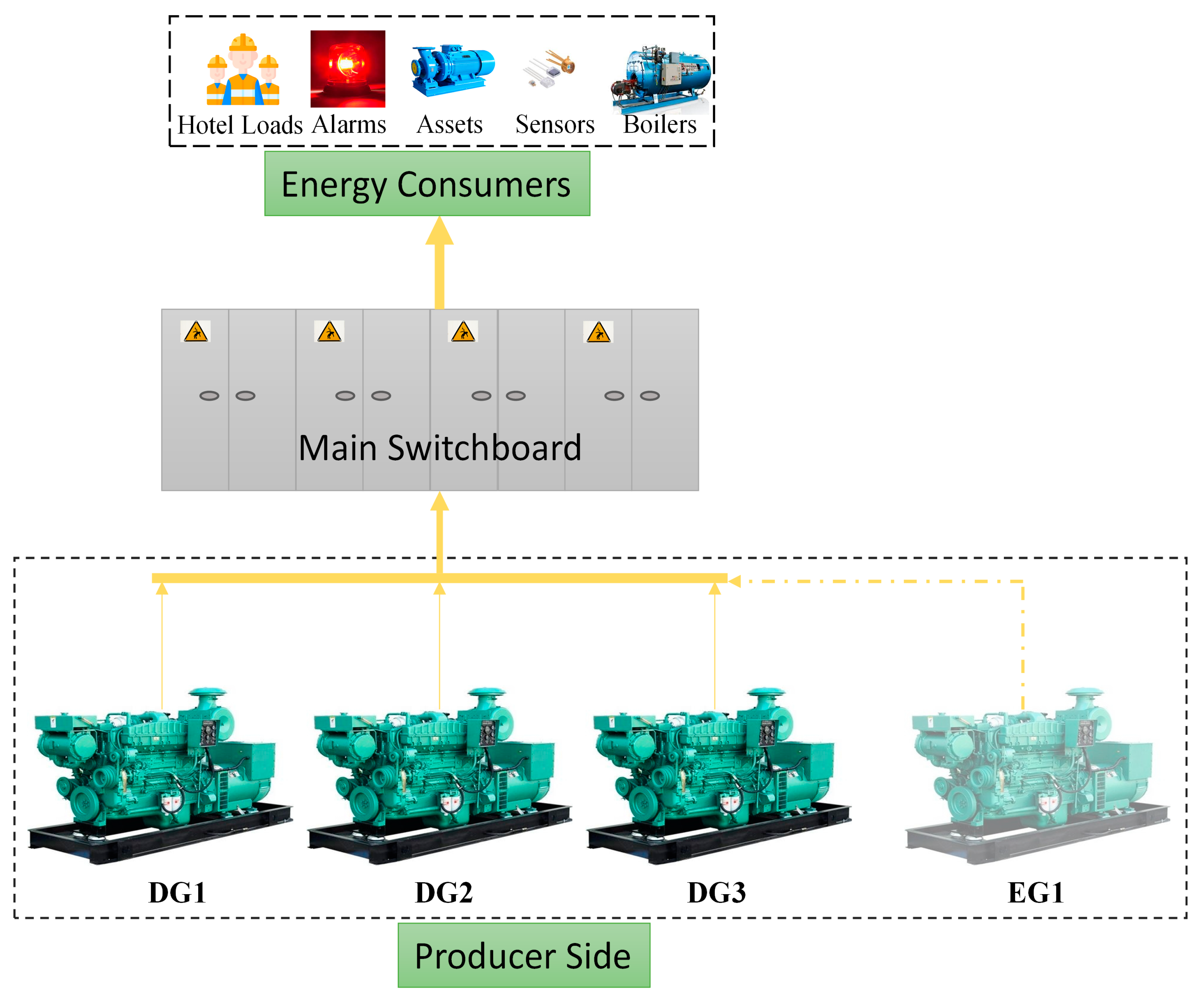
In this ship microgrid, diesel generators are the energy generators, while, hotel loads, alarms, pumps, sensors, and boilers, are the energy consumers. Figure 2 shows the general structure of the chemical tanker ship microgrid used in this case study. Three diesel generators power the entire shipload, while a fourth emergency generator is available in case of a main generator failure.

3.1. Data Processing

Data collection is the fundamental process in data-driven studies [29]. A solid and clean dataset can also facilitate the achievement of the targeted results in the study [30]. Initially, in this study, a 1461-day voyage dataset was gathered for investigation. Then, the sections of this dataset that had null values were eliminated, resulting in 1000 days of refined data that could be used in this study. The ship’s characteristics and the brief statistical information of the dataset are given in Table 1 and Table 2, respectively. The data features used in this study are as follows:
  • Main engine speed (revolutions per minute (rpm)).
  • Diesel generator fuel consumption (t/day), power (kW).
  • Main engine running hours (h/day).
  • Diesel generator running hours (h/day).
  • Main engine output maximum continuous rating (%).
  • Main engine power (kW), fuel consumption (t/day).
  • Fresh water generator running hours (h/day).
  • Scavenge air temperature (°C), scavenge pressure (bar).
  • Main engine exhaust temperature (°C).
  • Boiler running hours (h/day).
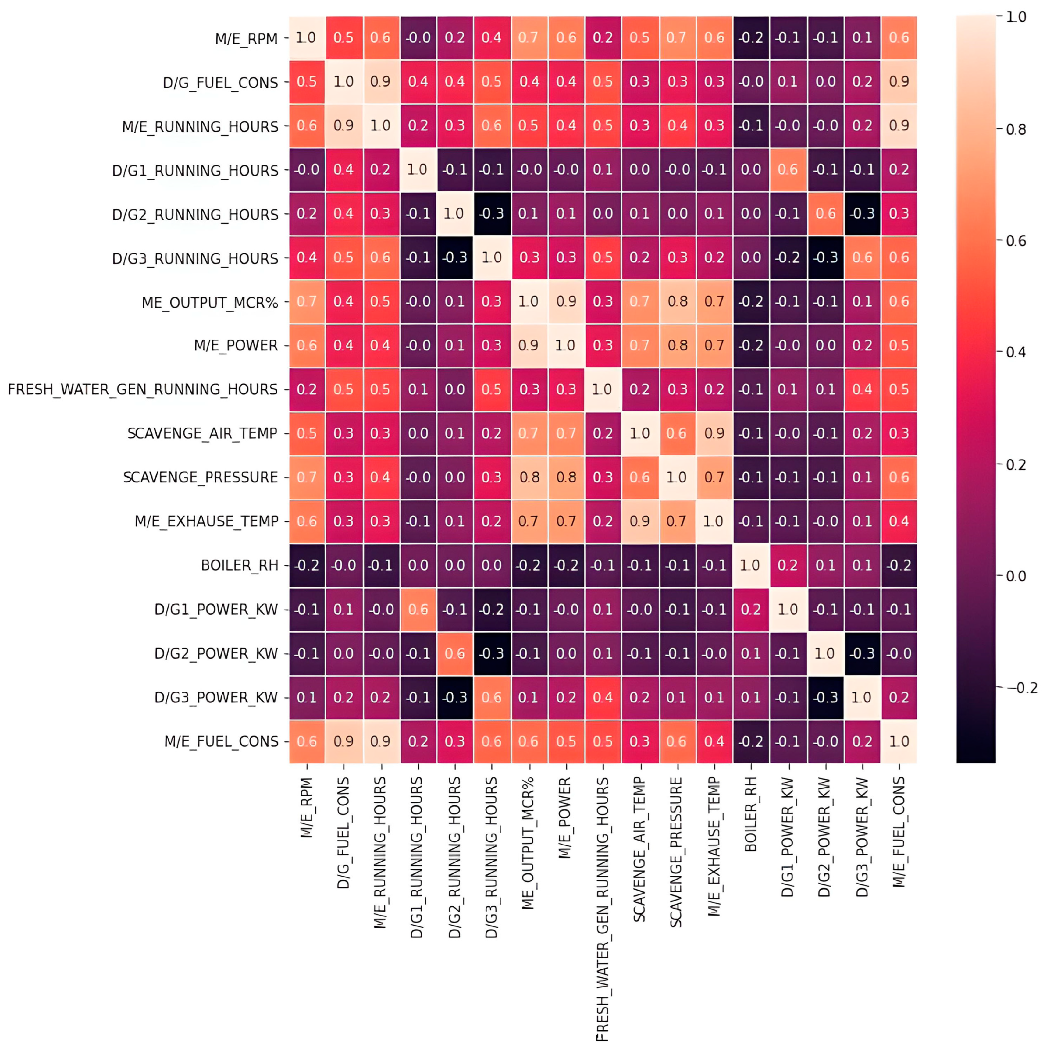
In data-driven studies, correlation analysis explains the relationship between the data and determines the variables. The Pearson correlation coefficient (r) was used to determine the relationship between two variables in the dataset. The correlation coefficient takes values between −1 and +1. Figure 3 shows the Pearson correlation matrix of the dataset. Here, the “+” sign in front of the correlation coefficient indicates a positive correlation between the two variables and the “−” sign indicates a negative correlation between the two variables. For example, in this dataset, diesel generators’ fuel consumption and the main engine fuel consumption values are strongly correlated (0.9), while diesel generator 1 running hours and the scavenge air temperature value correlation value is 0.
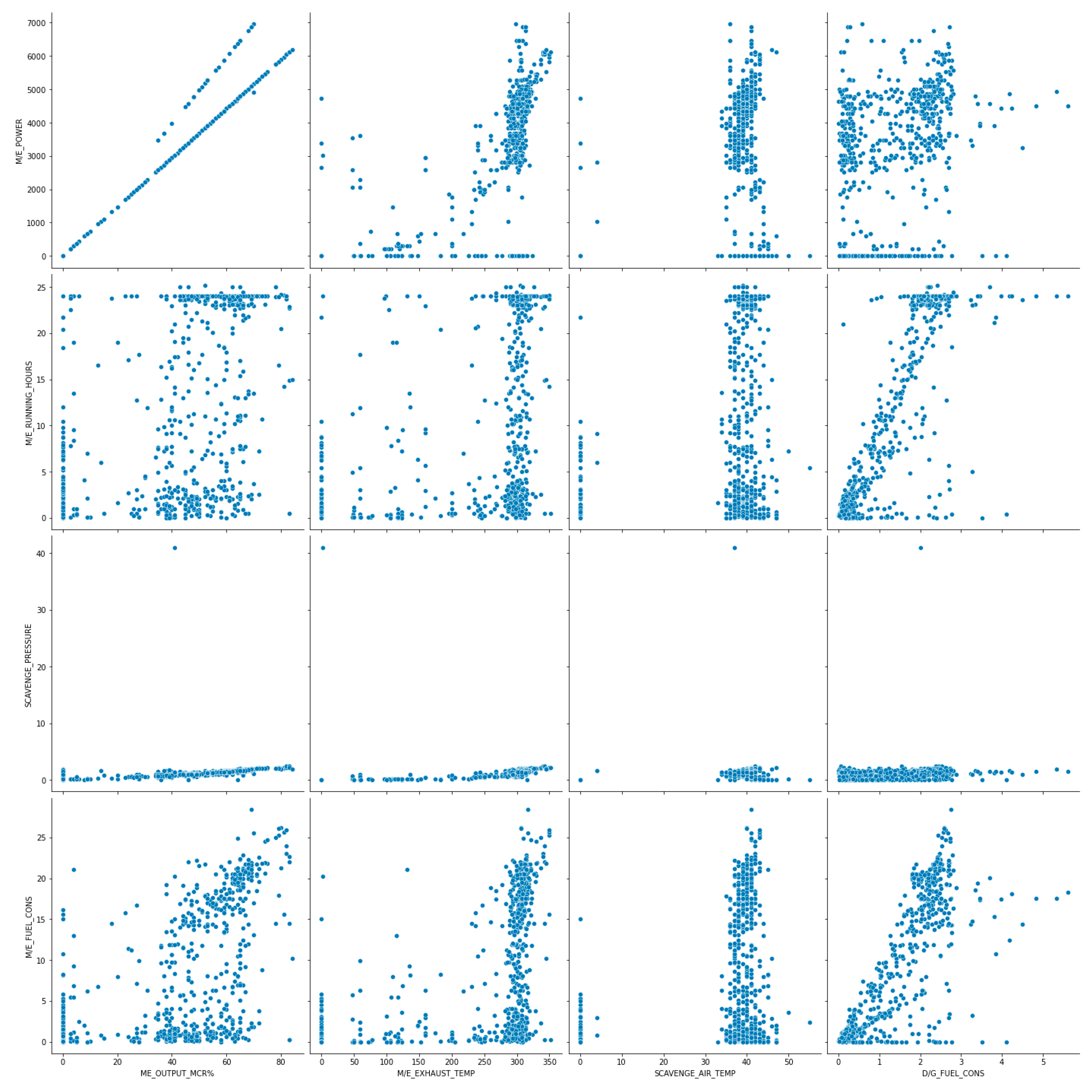
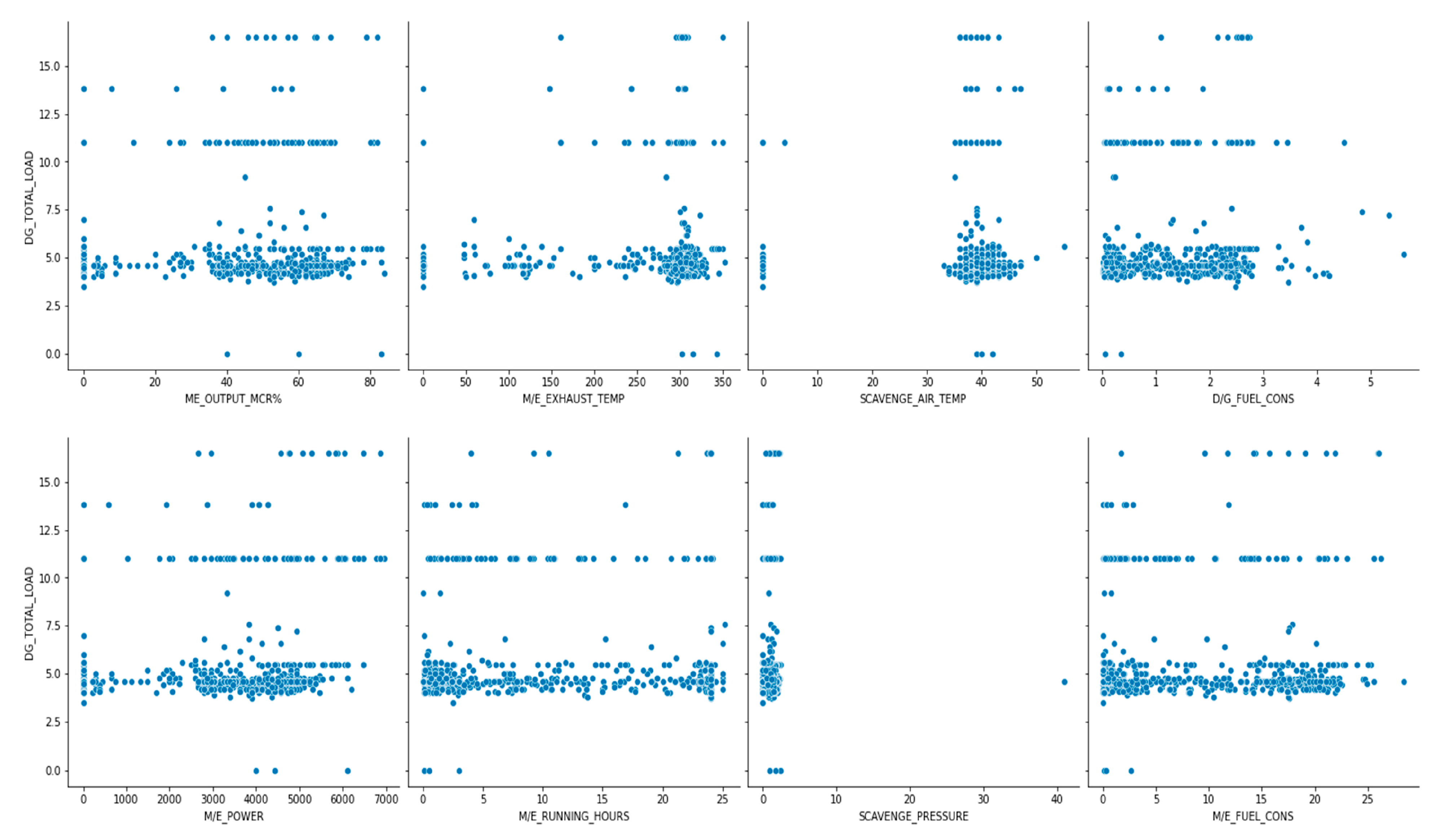
The pair plot method can enable a more detailed examination of the correlation between the variables in the dataset. The pair plot of the variables with a high correlation coefficient in this study is shown in Figure 4. The relationship between these variables and the total load of the generators is also shown in Figure 5. While the main engine and power variables show a strong correlation for all values, other variables cannot form such a linear graph. When Figure 5 is examined, it can be seen that the total load of the diesel generator shows a correlation within a specific range with the scavenge pressure variable.
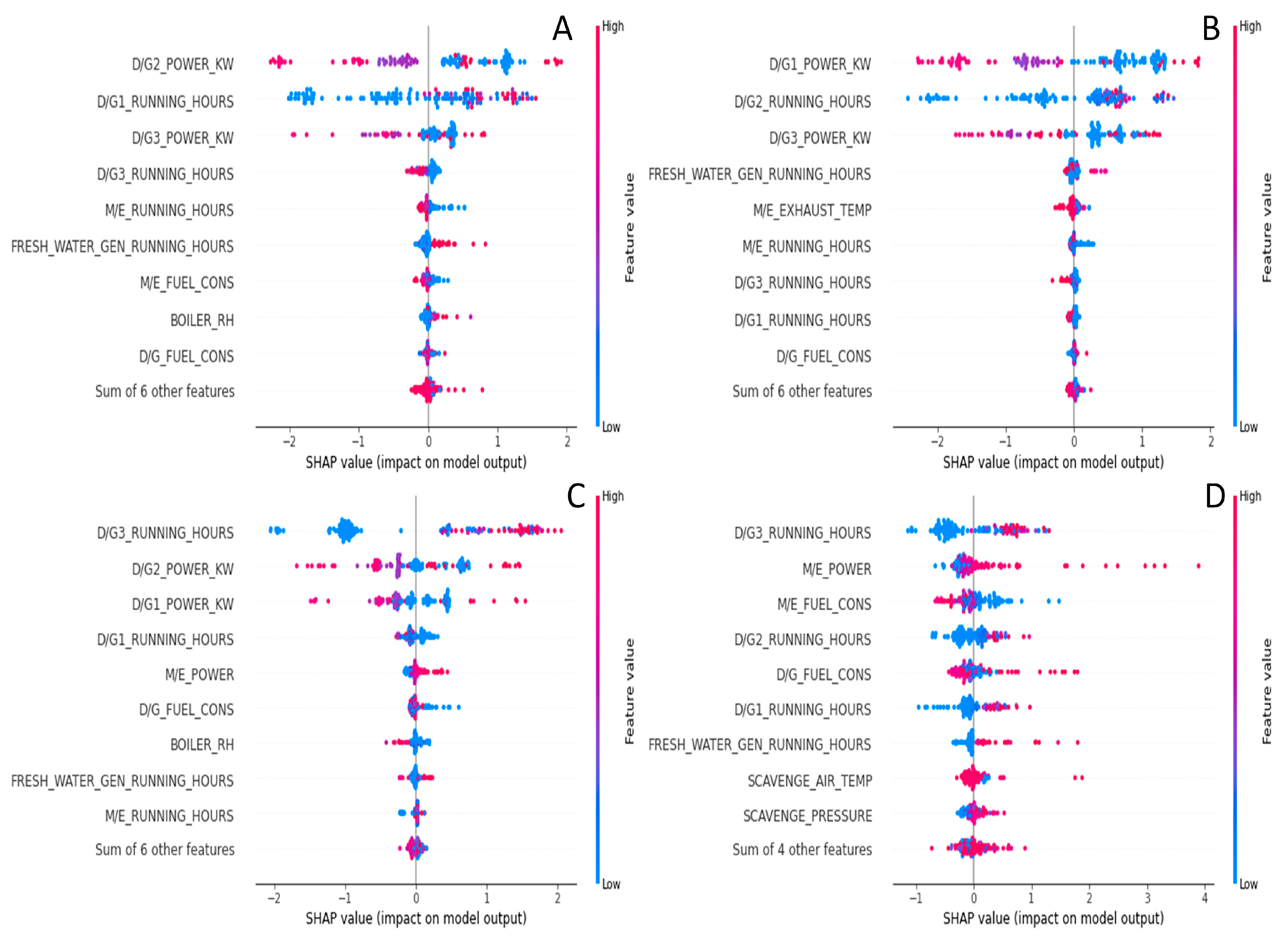
SHAP values (SHapley Additive exPlanations 3.7.7) follow a method that is based on game theory and enables the determination of the influence of inputs on the output variables in the dataset [31,32]. The SHAP values that were discovered quantified the importance of the inputs in determining the system’s output in this prediction model, and they are illustrated in Figure 6. Figure 6A shows the effect of input variables on the output while estimating the power of diesel generator 1. Figure 6B,C show how input variables affect output for generators 2 and 3, respectively. Meanwhile, Figure 6D shows the effect of the input variables on the output in the model used to estimate the total load of the generators. For the DG1 power prediction process (Figure 6A), it can be said that DG2 power, DG1 running hours, and DG3 power are more important than the other features in the dataset. Figure 6B shows that DG1 power, DG2 running hours, and DG3 power values are more important features for the DG2 power prediction phase. For the DG3 power prediction, DG3 running hours, DG2 power, and DG1 power values are more important than the other features (Figure 6C), and important values are presented in the Figure 6D for the total load prediction case.

3.2. Estimation Models

3.2.1. Support Vector Machines (SVM)

The support vector machine (SVM), developed by AT&T Bell Labs, is a supervised learning method frequently used in classification and regression problems. This algorithm has an effective usage area for accuracy, proper generalization, and precision theories [33]. In this method, the predicted results that fall within a given range are considered successful, whereas those that fall outside of that range are considered failed. Vectors that limit this range value are called support vectors [34]. The model of the SVM is given below.
f x = w T x + w 0
H w , w 0 = i = 1 N ( y i f ( x i ) ) + λ 2 w 2
V Ɛ r = 0   i f r < Ɛ r Ɛ   o t h e r w i s e
Here, w is the normal vector, x is an independent variable, λ is the regularisation parameter, w 0 is coefficient, V is the error function, Ɛ is the error margin, and r is the error [35]. Figure 7 describes the components of the support vector machine. The blue dots represent successful predictions within the permissible margin borders (support vectors), and it can be seen in the figure that the red dots show unsuccessful results or another cluster [19].

3.2.2. Multiple Linear Regression (MLR)

The multiple linear regression (MLR) method is a statistical technique that consists of dependent and independent variables. In this method, dependent variables can be calculated with the help of more than one independent variable and coefficient [36,37]. Multiple linear regression can be expressed by Equation (4),
y = a 0 + a 1 x 1 + + a n x n + Ɛ
where a 0 , a 1 , , a n are coefficients, y is the dependent variable, Ɛ is the model error, and x 1 , x 2 , , x n are independent variables. In this method, a n (coefficients) are calculated using Equation (5).
a n = a r g m i n ( a ) i = 1 n ( y i a 0 j = 1 n a j x i j ) 2

3.2.3. Artificial Neural Network (ANN)

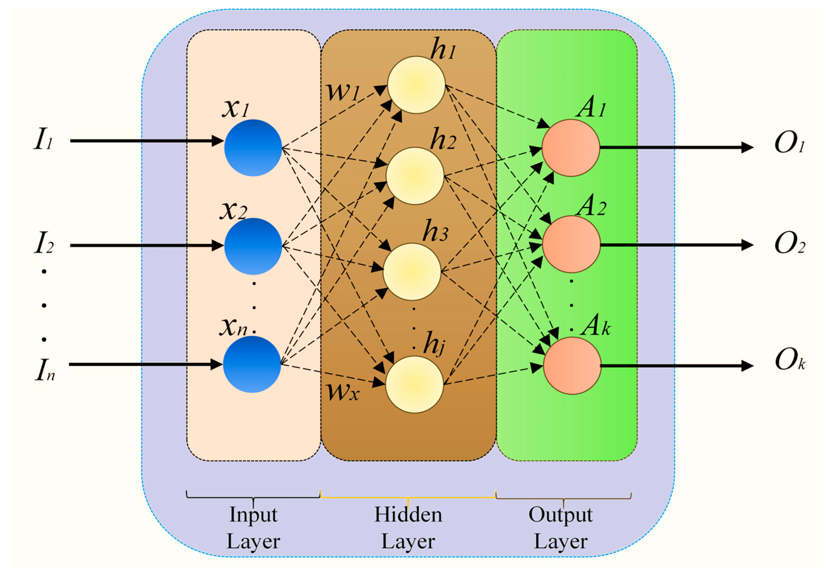
The artificial neural network method, which imitates the working process of the brain, is a structure consisting of artificial neurons and nodes [38]. In this structure, neurons receive and process the signal and transmit it to other neurons with which it is connected. The signal formed in this structure is the sum of the signals coming from the connected neurons [34]. Other considerations in artificial neural networks are the weight variables and the activation function [39]. The weight variable affects the value of the output function by increasing or decreasing the strength of a signal in the neural network. The activation function, on the other hand, determines how the output signal, which is determined by the weights, will be transferred from a certain layer of the network to another layer or the output of the network. A typical artificial neural network is represented in Figure 8. When the figure is examined, I values represent the input values of the network, while X values form the input layer. Here, h values create the hidden layer, while A values create the output layer. O values represent the output values of the network. In addition, the w values in the figure represent the weights [39,40,41,42].

3.2.4. Deep Neural Network (DNN)

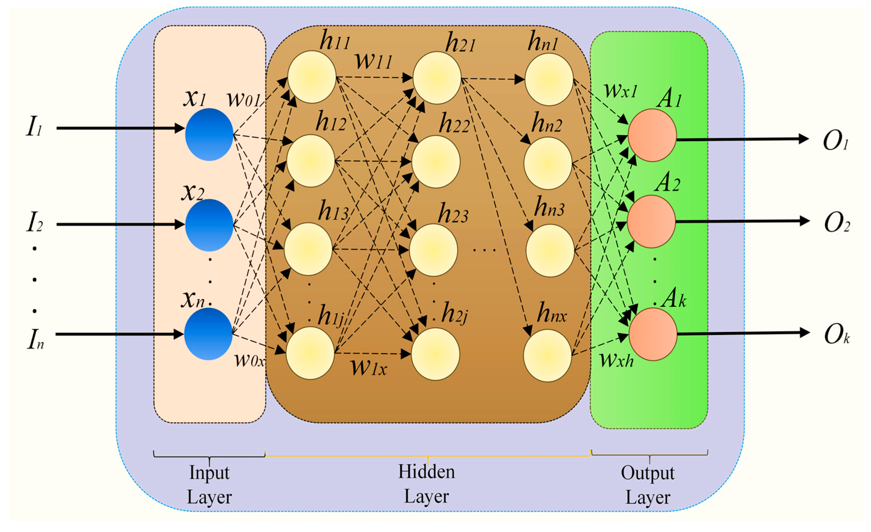
A deep neural network can be defined as an advanced ANN structure [43,44]. This method has the same weight and activation functions as an ANN structure, but it differs in the number of hidden layers. In this way, much more parameter optimization can be made in the deep neural network structure, and more successful results can be obtained [45]. A typical DNN structure is shown in Figure 9. When Figure 9 is examined, I values form the inputs, x values form the input layer, w values form the weights, and h values form the hidden layer. Values form the output layer, while O values are the output values of the system [46,47].

3.2.5. K-Nearest Neighbours (KNN)

The k-nearest neighbours algorithm is based on the principle of determining the distance of k-nearest neighbours to a certain point [48]. Here, the k parameter may vary according to the model [49,50]. While making predictions with the KNN algorithm, the model continues training by making use of past data. Minkowski distance (Lp), an important parameter used in this algorithm, is used for the specification of the margin between a start point (xq) and any other point (xj) (Equation (6)).
L p x j , x q = i | x j , i x q , i | p 1 p
Here, if p = 1 is the Manhattan distance, p = 2 is the Euclidean distance [51].

3.2.6. Random Forest (RF)

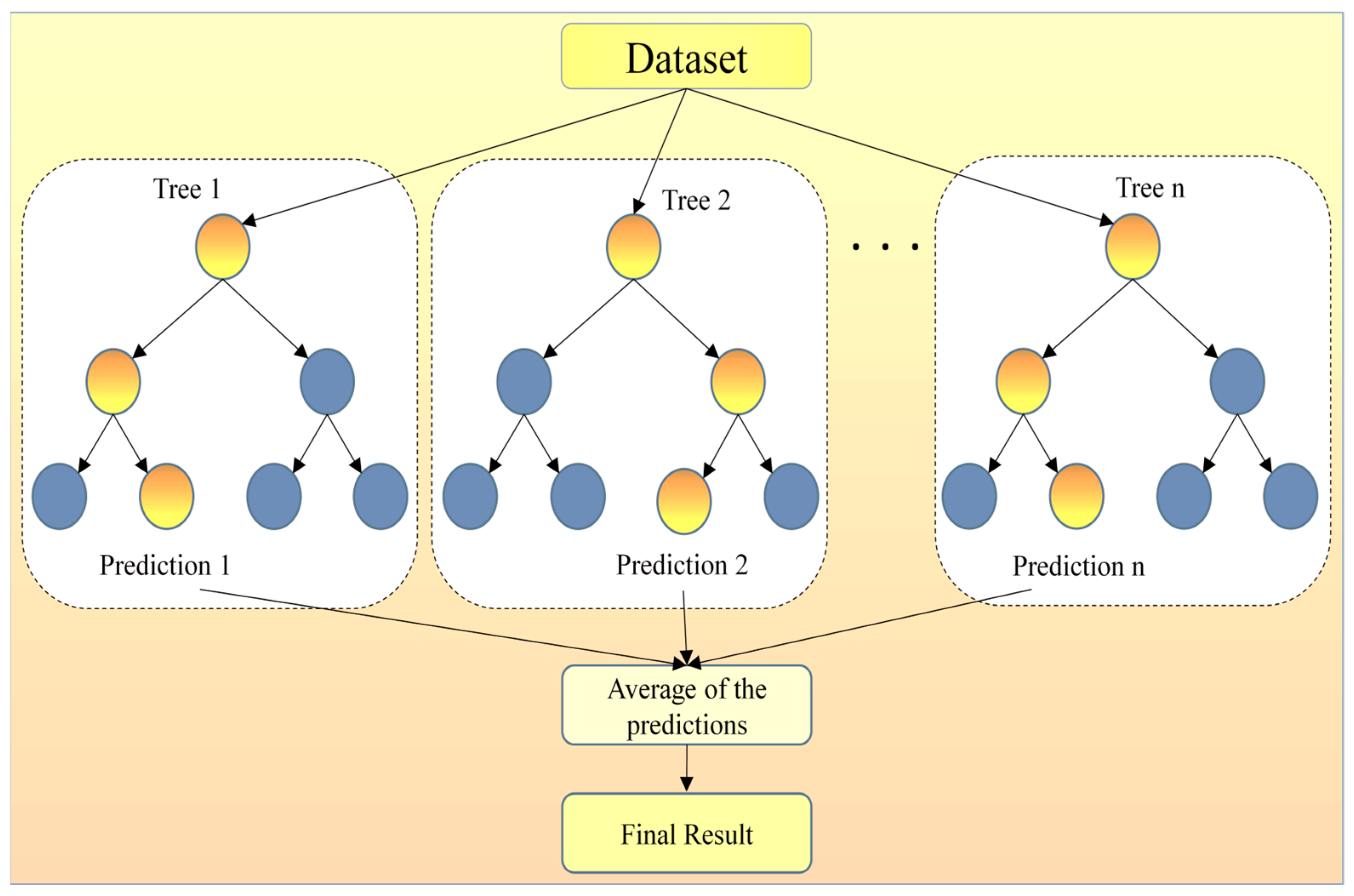
In the random forest (RF) algorithm, an advanced form of the decision tree algorithm, the results are obtained through multiple decision trees [52]. When used for classification purposes, the output produced by the most trees is considered the final result. In contrast, the average results obtained from all of the trees in regression problems give the final result [53]. A typical RF structure is presented in Figure 10.

3.2.7. Extreme Gradient Boosting (XGBoost)

The extreme gradient boosting method is an approach that uses a decision tree and gradient boosting structure [54]. In this approach, the value obtained by summing the results from the decision tree algorithm is f(x), and the model equation is as follows (Equation (7)) [55].
ŷ i = j = 1 N f j ( x i )
The XGBoost algorithm advances by making improvements to the objective function, whose main task is to optimize the complexity penalty and loss function. Here, the loss function (LF) is expressed in Equation (8) and the complexity penalty (CP) in Equation (9) [56].
L F = i = 1 n l ( y i , ŷ i )
C P = k k Ω ( f k )

3.2.8. Decision Tree Regressor (DTree)

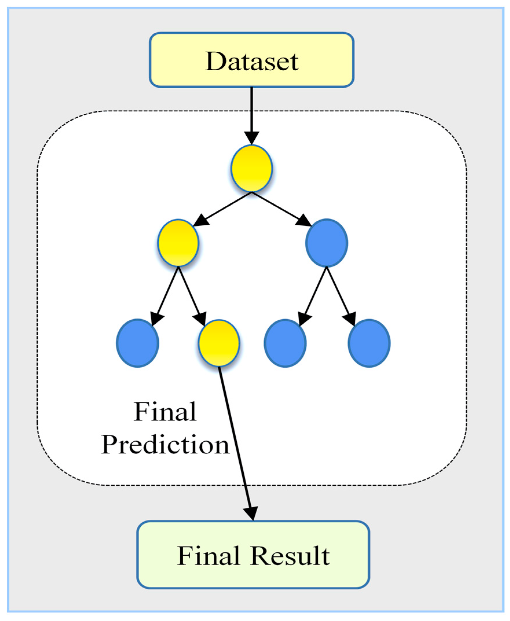
The decision tree algorithm is a supervised machine learning method that is frequently used in regression and classification problems in the literature because they are generally understandable and practical [57]. In regression problems, if the target variable takes continuous values, the decision tree regressor can be used at this stage. During the estimation process, the dataset is iteratively partitioned and the algorithm runs until the partitioning process stops [58]. The decision tree method can be divided into decision nodes, branches, and leaves. A simple decision tree model is shown in Figure 11 [20].

3.3. Validation and Evaluation

3.3.1. Mean Absolute Error (MAE)

Mean absolute error (MAE) is an error metric found by calculating the average absolute values of the distances between the actual and predicted values [59,60]. Calculation of the mean absolute error is shown in Equations (10) and (11).
M A E = 1 N i = 1 N e i
e i = a i p i
Here, e i is an error value, a i is the actual value, and p i is the predicted value.

3.3.2. Root Mean Square Error (RMSE)

Root mean square error (RMSE) is a measure of the distance between values predicted by a model and actual values. It is calculated by taking the square root of the mean of the square of the difference between the actual values and the predicted values [25,59]. The calculation of RMSE is given in Equation (12),
R M S E = i = 1 N e i 2 N
where e i = a i p i represents the error value, a i is the actual value, p i is the predicted value, and N is amount of data.

3.3.3. Mean Absolute Percentage Error (MAPE)

The mean absolute percentage error (MAPE) is the percentage of difference between actual and predicted values. The calculation of MAPE is expressed in Equation (13) [61].
M A P E = 100 % n i = 1 n y i p i y i
In this equation, y is the actual value and p is the predicted value.

3.3.4. K-Fold Cross-Validation

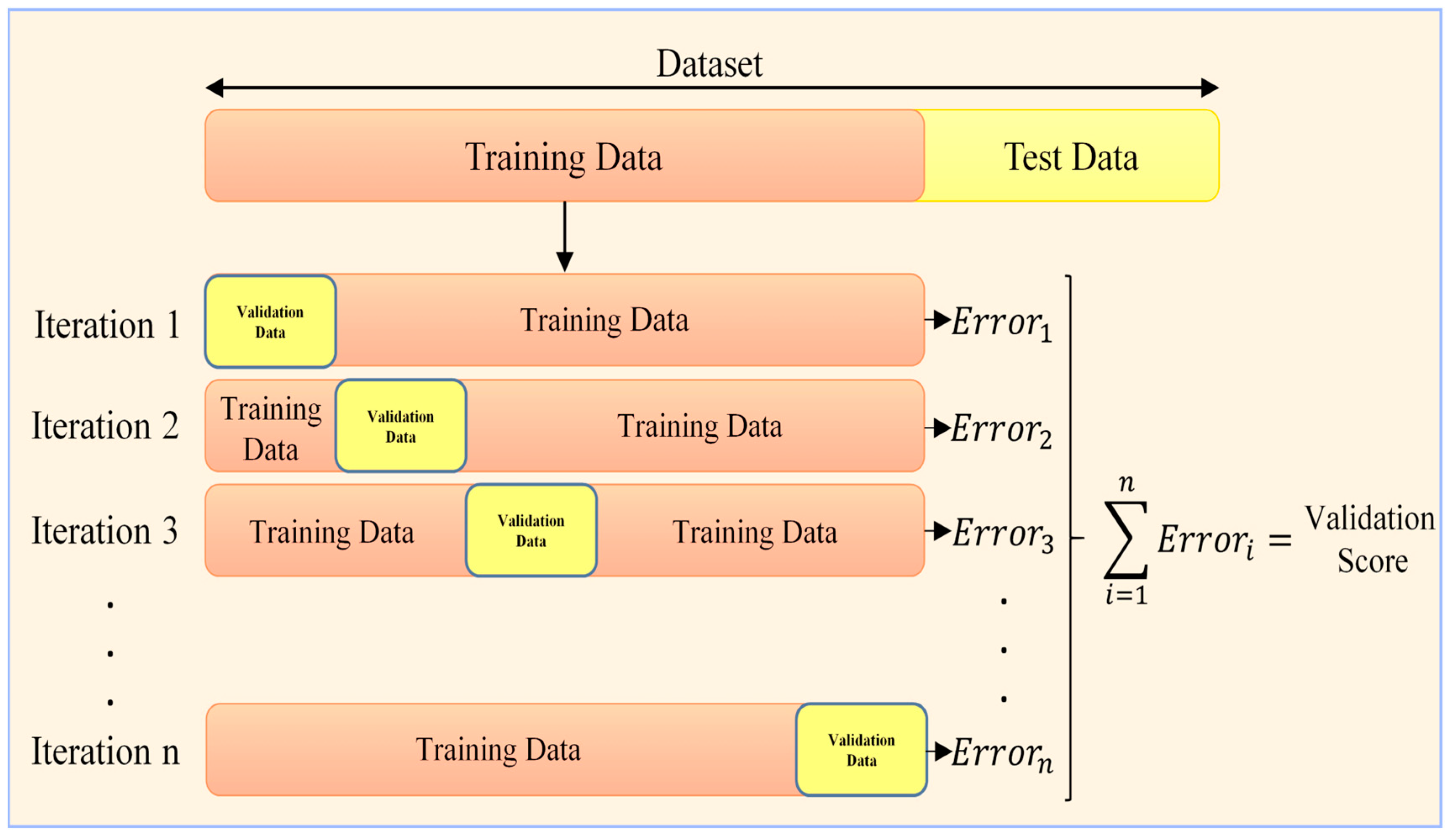
K-fold cross-validation is a verification method in which algorithms are checked for overfitting problems [62]. In this method, the dataset is divided into equal parts; one test is divided for validation and the other parts are separated as training data. The validation process continues until all parts are processed, and the average of the results obtained is calculated as the validation score [60]. The k-fold cross-validation process is described in Figure 12.

4. Simulation Results and Discussion

Achieving generator load prediction output values that are close to the real values is the main objective of the proposed training model. A forecasting model that produces the lowest rate of error demonstrates a high prediction accuracy and is capable of generating reliable results for new sets of data. In order to figure out the prediction model for a data-driven approach that can satisfy the prediction objective, eight different algorithms were utilized, which are SVM, MLR, ANN, DNN, KNN, RF, XGB, and Dtree. The comparative results from all of the algorithms provide the best prediction model for the generator load of the chemical tanker. The findings from the analysis of each prediction model’s performance are addressed in this section.
This study used the TensorFlow environment of Python programming language version 3.7.7 in simulations for marine diesel generator power prediction. The computer hardware utilized an Intel Core i7-9750H 2.60 GHz processor, 32 GB of RAM, and an NVIDIA GeForce RTX 2070 graphics card. In the first stage of the simulation, the hyperparameters of the established models were tuned since some of the algorithms were unable to produce the desired prediction scores. Hyperparameter tuning has the advantage of providing optimized values for the prediction model, maximizing the predictive accuracy as much as possible. This is an essential step in controlling the behaviour of the predictive model. Without the hyperparameter tuning step, the prediction model will make more errors during the data simulation. Table 3 shows the model hyperparameters obtained as a result of this process.
The performance of each prediction algorithm was evaluated by several error metrics such as MAE, RMSE, and MAPE. In the first scenario, the prediction model was conducted for each generator of DG1, DG2, and DG3 separately.
Table 4 compares the results of the eight prediction algorithms for the power prediction in each generator. It shows that the decision tree (Dtree) algorithm is more efficient than the other algorithms used for this specific case study. It reached values of 0.2364 for MAE, 0.2455 for RMSE, and 17.493 for MAPE for the DG1 power prediction case. When DG2 power prediction scores were evaluated, the DTree algorithm reached values of 0.1306 for MAE, 0.2069 for RMSE, and 5.1139 for MAPE. For DG3 power prediction, the DTree algorithm reached values of 0.1532 for MAE, 0.2182 for RMSE, and 7.7481 for MAPE. The DTree algorithm is a typical model-based learning method. The difference of this method from other algorithms is the modelling of the relationship between the input variables and the output variable. For this reason, it can achieve successful results in both linear and nonlinear systems [63]. On the other hand, XGB, RF, and DNN also show a good performance, with their error measurement performing slightly better than Dtree’s. Meanwhile, the SVR technique has the worst performance with the highest error rate. This could be due to it performing operations with a margin between hyperplanes that allows a certain degree of error. Meanwhile, the other prediction algorithm is intended to minimize the error rate as much as possible. That justifies the highest error performance for the case study.
Knowing the effects of loads on generators can assist maritime companies in predicting malfunctions, improving energy efficiency, and conducting maintenance-attitude studies [64]. When the generator load is known, the fuel consumption can be calculated. In this way, fuel consumption can be optimized, and steps can be taken toward greater energy efficiency [65]. Knowing the fuel consumption can also enable the detection of a malfunction or an error in the generator system when the consumption differs from the normal state, i.e., when the energy efficiency changes. This can help shipping companies in terms of predictive maintenance activities.
In the second scenario, the total load power generator prediction model was developed by taking into account all of the chemical tanker ship’s generators. Table 5 shows the prediction results for the total load estimation from eight prediction models. To determine whether the models were overfitting, a 5-fold cross-validation procedure was used. The training dataset was divided into five parts with 200 samples each in this process; one of these parts was designated as the validation dataset, while the other four were used as training data in the model training. The cross-validation process was continued for five iterations, and the validation scores are given in Table 6 in terms of the mean absolute error metric.
In this case, the deep neural network (DNN) algorithm outperforms all other algorithms, with minimum error performance values of 1.0866 (MAE), 2.6049 (RMSE), and 14.728 (MAPE). In light of the findings obtained in the first simulation study, it was revealed that model-based algorithms for the generator power estimation case phase are more advantageous due to the format of the dataset. In addition, it can be said that the XGBoost algorithm, which uses a progressive learning methodology, stands out among other algorithms used in the simulation process. In the second part of the simulation study, concerning the prediction of the total load of the generators, it was revealed that the DNN algorithm, which works more efficiently in difficult and complex systems, achieves more successful prediction scores than other algorithms. Unlike ANN, there are multiple hidden layers in DNN. This allows the algorithm to behave more effectively in more complex problems. In addition, the DNN algorithm is also a successful method for nonlinear systems. At this stage, reducing the number of inputs of the system significantly reduced the success of the models established with MLR, ANN, K-NN, RF, XGBoost, and DTree algorithms. However, the DNN and SVR algorithms improved their scores in this process. When the DNN and SVR algorithms were compared, it was determined that the success of the DNN algorithm increased significantly in the second simulation. It can be observed that the success of the SVR algorithm also increased, but this increase was not at a satisfactory level.

5. Conclusions

Generators are the second-largest fuel consumer on a ship after the primary engine and, thus, are an important component when evaluating fuel utilization and enhancing energy efficiency. If the electrical load on the generators cannot be correctly predicted and planned for, electrical failures may also occur under sudden loads. This issue may force the ship’s operations to cease and might result in the ship’s severe damage and workplace accidents. This study employed data-driven algorithms to estimate the load on a commercial ship’s generators. The results from the simulation indicated that the DTree model was the most successful method for the generator load prediction, with MAE scores of 0.2364, 0.1306, and 0.1532; RMSE scores of 0.2455, 0.2069, and 0.2182; and MAPE scores of 17.493, 5.1139, and 7.748 for diesel generators DG1, DG2, and DG3, respectively. On the other hand, the DNN model was the most successful method for the total load prediction case, with 1.0866 MAE, 2.6049 RMSE, and 14.728 MAPE scores. The 5-iteration k-fold cross-validation procedure used to determine whether the models had an overfitting condition revealed no overfitting condition.
It can be concluded from the results that data-driven algorithms can be useful for estimating the electrical load on ship generators. The problems arising from the sudden loads experienced in the ship’s electrical grid may be prevented by injecting these developed models in this study into the ship microgrid control in the future. This will make it possible to take preventative action against electrical failures, prevent potential malfunctions, reduce potential additional maintenance costs, and increase energy efficiency.

Author Contributions

T.U.: Conceptualization, Methodology, Software, Validation, Formal analysis, Writing—original draft, N.N.A.B.: Conceptualization, Methodology, Validation, Writing—review & editing, Writing—original draft, Ö.K. and Y.A.: Supervision, Investigation, Writing—review & editing, Writing—original draft, J.M.G. and A.L.: Supervision, Writing—review & Editing. All authors have read and agreed to the published version of the manuscript.

Funding

This work was supported by The Scientific and Technological Research Council of Turkey BIDEB 2214-A International Doctoral Research Fellowship Programme reference number:1059B142100334. Josep M. Guerrero and Abderezak Lashab are funded by VILLUM FONDEN under the VILLUM Investigator Grant (25920): Center for Research on Microgrids (CROM).

Institutional Review Board Statement

Not applicable.

Informed Consent Statement

Not applicable.

Data Availability Statement

Not applicable.

Acknowledgments

This work was supported by the Scientific and Technological Research Council of Turkey BIDEB- 2214 International Doctoral Research Fellowship Programme. This article is produced from the PhD dissertation entitled “Deep Learning Applications in Ship Electric Grids” which has been executed in the Maritime Transportation Engineering Program of ITU Graduate School.

Conflicts of Interest

The authors declare no conflict of interest.

References

  1. Sáez Álvarez, P. From Maritime Salvage to IMO 2020 Strategy: Two Actions to Protect the Environment. Mar. Pollut. Bull. 2021, 170, 112590. [Google Scholar] [CrossRef] [PubMed]
  2. Ammar, N.R.; Seddiek, I.S. Enhancing Energy Efficiency for New Generations of Containerized Shipping. Ocean Eng. 2020, 215, 107887. [Google Scholar] [CrossRef]
  3. Bakar, N.N.A.; Bazmohammadi, N.; Çimen, H.; Uyanik, T.; Vasquez, J.C.; Guerrero, J.M. Data-Driven Ship Berthing Forecasting for Cold Ironing in Maritime Transportation. Appl. Energy 2022, 326, 119947. [Google Scholar] [CrossRef]
  4. Gan, M.; Hou, H.; Wu, X.; Liu, B.; Yang, Y.; Xie, C. Machine Learning Algorithm Selection for Real-Time Energy Management of Hybrid Energy Ship. Energy Rep. 2022, 8, 1096–1102. [Google Scholar] [CrossRef]
  5. Pagoropoulos, A.; Møller, A.H.; McAloone, T.C. Applying Multi-Class Support Vector Machines for Performance Assessment of Shipping Operations: The Case of Tanker Vessels. Ocean Eng. 2017, 140, 1–6. [Google Scholar] [CrossRef] [Green Version]
  6. Planakis, N.; Papalambrou, G.; Kyrtatos, N. Ship Energy Management System Development and Experimental Evaluation Utilizing Marine Loading Cycles Based on Machine Learning Techniques. Appl. Energy 2022, 307, 118085. [Google Scholar] [CrossRef]
  7. Hou, J.; Sun, J.; Hofmann, H. Adaptive Model Predictive Control with Propulsion Load Estimation and Prediction for All-Electric Ship Energy Management. Energy 2018, 150, 877–889. [Google Scholar] [CrossRef]
  8. Hardan, F.; Norman, R. Balancing Loads of Rotating Generators Utilizing VSC Direct Power Controllers in a Ship AC/DC Smartgrid. Electr. Power Syst. Res. 2020, 182, 106200. [Google Scholar] [CrossRef]
  9. Omer, H.A.; Mahjoub, K.O.; Karrar, A.A. On the Stability of Generators Load Sharing; IFAC: New York, NY, USA, 2014; Volume 19, ISBN 9783902823625. [Google Scholar]
  10. Roy, N.B.; Das, D. Optimal Allocation of Active and Reactive Power of Dispatchable Distributed Generators in a Droop Controlled Islanded Microgrid Considering Renewable Generation and Load Demand Uncertainties. Sustain. Energy Grids Netw. 2021, 27, 100482. [Google Scholar] [CrossRef]
  11. Kusakana, K. Optimal Peer-to-Peer Energy Sharing between Prosumers Using Hydrokinetic, Diesel Generator and Pumped Hydro Storage. J. Energy Storage 2019, 26, 101048. [Google Scholar] [CrossRef]
  12. Li, X.; Sun, B.; Jin, J.; Ding, J. Speed Optimization of Container Ship Considering Route Segmentation and Weather Data Loading: Turning Point-Time Segmentation Method. J. Mar. Sci. Eng. 2022, 10, 1835. [Google Scholar] [CrossRef]
  13. Uyanık, T.; Yalman, Y.; Kalenderli, Ö.; Arslanoğlu, Y.; Terriche, Y.; Su, C.-L.; Guerrero, J.M. Data-Driven Approach for Estimating Power and Fuel Consumption of Ship: A Case of Container Vessel. Mathematics 2022, 10, 4167. [Google Scholar] [CrossRef]
  14. Bassam, A.M.; Phillips, A.B.; Turnock, S.R.; Wilson, P.A. Ship Speed Prediction Based on Machine Learning for Efficient Shipping Operation. Ocean Eng. 2022, 245, 110449. [Google Scholar] [CrossRef]
  15. Murray, B.; Perera, L.P. Proactive Collision Avoidance for Autonomous Ships: Leveraging Machine Learning to Emulate Situation Awareness. IFAC Pap. 2021, 54, 16–23. [Google Scholar] [CrossRef]
  16. Rawson, A.; Brito, M.; Sabeur, Z.; Tran-Thanh, L. A Machine Learning Approach for Monitoring Ship Safety in Extreme Weather Events. Saf. Sci. 2021, 141, 105336. [Google Scholar] [CrossRef]
  17. Peng, Y.; Liu, H.; Li, X.; Huang, J.; Wang, W. Machine Learning Method for Energy Consumption Prediction of Ships in Port Considering Green Ports. J. Clean. Prod. 2020, 264, 121564. [Google Scholar] [CrossRef]
  18. Anh Tran, T. Comparative Analysis on the Fuel Consumption Prediction Model for Bulk Carriers from Ship Launching to Current States Based on Sea Trial Data and Machine Learning Technique. J. Ocean Eng. Sci. 2021, 6, 317–339. [Google Scholar] [CrossRef]
  19. Ahlgren, F.; Mondejar, M.E.; Thern, M. Predicting Dynamic Fuel Oil Consumption on Ships with Automated Machine Learning. Energy Procedia 2019, 158, 6126–6131. [Google Scholar] [CrossRef]
  20. Uyanık, T.; Karatuğ, Ç.; Arslanoğlu, Y. Machine Learning Approach to Ship Fuel Consumption: A Case of Container Vessel. Transp. Res. Part D Transp. Environ. 2020, 84, 102389. [Google Scholar] [CrossRef]
  21. Kong, M.C.; Roh, M.-I.; Kim, K.S.; Lee, J.; Kim, J.; Lee, G. Object Detection Method for Ship Safety Plans Using Deep Learning. Ocean Eng. 2022, 246, 110587. [Google Scholar] [CrossRef]
  22. Laurie, A.; Anderlini, E.; Dietz, J.; Thomas, G. Machine Learning for Shaft Power Prediction and Analysis of Fouling Related Performance Deterioration. Ocean Eng. 2021, 234, 108886. [Google Scholar] [CrossRef]
  23. Saettone, S.; Tavakoli, S.; Taskar, B.; Jensen, M.V.; Pedersen, E.; Schramm, J.; Steen, S.; Andersen, P. The Importance of the Engine-Propeller Model Accuracy on the Performance Prediction of a Marine Propulsion System in the Presence of Waves. Appl. Ocean Res. 2020, 103, 102320. [Google Scholar] [CrossRef]
  24. Wen, H.; Khan, F.; Amin, M.T.; Halim, S.Z. Myths and Misconceptions of Data-Driven Methods: Applications to Process Safety Analysis. Comput. Chem. Eng. 2021, 158, 107639. [Google Scholar] [CrossRef]
  25. Lang, X.; Wu, D.; Mao, W. Comparison of Supervised Machine Learning Methods to Predict Ship Propulsion Power at Sea. Ocean Eng. 2022, 245, 110387. [Google Scholar] [CrossRef]
  26. Zhou, T.; Hu, Q.; Hu, Z.; Zhen, R. An Adaptive Hyper Parameter Tuning Model for Ship Fuel Consumption Prediction under Complex Maritime Environments. J. Ocean Eng. Sci. 2021, 7, 255–263. [Google Scholar] [CrossRef]
  27. Yan, R.; Wang, S.; Du, Y. Development of a Two-Stage Ship Fuel Consumption Prediction and Reduction Model for a Dry Bulk Ship. Transp. Res. Part E Logist. Transp. Rev. 2020, 138, 101930. [Google Scholar] [CrossRef]
  28. Yuan, Z.; Liu, J.; Zhang, Q.; Liu, Y.; Yuan, Y.; Li, Z. Prediction and Optimisation of Fuel Consumption for Inland Ships Considering Real-Time Status and Environmental Factors. Ocean Eng. 2021, 221, 108530. [Google Scholar] [CrossRef]
  29. Schäfers, P.; Mütze, A.; Nyhuis, P. Integrated Concept for Acquisition and Utilization of Production Feedback Data to Support Production Planning and Control in the Age of Digitalization. Procedia Manuf. 2019, 31, 225–231. [Google Scholar] [CrossRef]
  30. Ellingsen, O.; Aasland, K.E. Digitalizing the Maritime Industry: A Case Study of Technology Acquisition and Enabling Advanced Manufacturing Technology. J. Eng. Technol. Manag. JETM 2019, 54, 12–27. [Google Scholar] [CrossRef]
  31. Futagami, K.; Fukazawa, Y.; Kapoor, N.; Kito, T. ScienceDirect Pairwise Acquisition Prediction with SHAP Value Interpretation. J. Financ. Data Sci. 2021, 7, 22–44. [Google Scholar] [CrossRef]
  32. Wang, D.; Thun, S.; Lindberg, U.; Jiang, L.; Trygg, J.; Tysklind, M. Towards Better Process Management in Wastewater Treatment Plants: Process Analytics Based on SHAP Values for Tree-Based Machine Learning Methods. J. Environ. Manag. 2022, 301, 113941. [Google Scholar] [CrossRef]
  33. Corinna, C.; Vladimir, V. Support-Vector Networks. IEEE Expert Syst. Appl. 1992, 7, 63–72. [Google Scholar] [CrossRef]
  34. Luíza da Costa, N.; Dias de Lima, M.; Barbosa, R. Evaluation of Feature Selection Methods Based on Artificial Neural Network Weights. Expert Syst. Appl. 2021, 168, 114312. [Google Scholar] [CrossRef]
  35. Liu, M.; Zhou, Q.; Wang, X.; Yu, C.; Kang, M. Voyage Performance Evaluation Based on a Digital Twin Model. IOP Conf. Ser. Mater. Sci. Eng. 2020, 929, 012027. [Google Scholar] [CrossRef]
  36. Xie, X.; Wu, T.; Zhu, M.; Jiang, G.; Xu, Y.; Wang, X.; Pu, L. Comparison of Random Forest and Multiple Linear Regression Models for Estimation of Soil Extracellular Enzyme Activities in Agricultural Reclaimed Coastal Saline Land. Ecol. Indic. 2021, 120, 106925. [Google Scholar] [CrossRef]
  37. Caravaggi, P.; Leardini, A.; Giacomozzi, C. Multiple Linear Regression Approach for the Analysis of the Relationships between Joints Mobility and Regional Pressure-Based Parameters in the Normal-Arched Foot. J. Biomech. 2016, 49, 3485–3491. [Google Scholar] [CrossRef] [PubMed]
  38. Hosseini, S.A.; Shirani, A.S.; Lotfi, M.; Menhaj, M.B. Design and Application of Supervisory Control Based on Neural Network PID Controllers for Pressurizer System. Prog. Nucl. Energy 2020, 130, 103570. [Google Scholar] [CrossRef]
  39. Jeon, M.; Noh, Y.; Shin, Y.; Lim, O.K.; Lee, I.; Cho, D. Prediction of Ship Fuel Consumption by Using an Artificial Neural Network. J. Mech. Sci. Technol. 2018, 32, 5785–5796. [Google Scholar] [CrossRef]
  40. Maepa, F.; Smith, R.S.; Tessema, A. Support Vector Machine and Artificial Neural Network Modelling of Orogenic Gold Prospectivity Mapping in the Swayze Greenstone Belt, Ontario, Canada. Ore Geol. Rev. 2021, 130, 103968. [Google Scholar] [CrossRef]
  41. Lazakis, I.; Raptodimos, Y.; Varelas, T. Predicting Ship Machinery System Condition through Analytical Reliability Tools and Artificial Neural Networks. Ocean Eng. 2018, 152, 404–415. [Google Scholar] [CrossRef] [Green Version]
  42. Choi, S.; Kim, Y.J. Artificial Neural Network Models for Airport Capacity Prediction. J. Air Transp. Manag. 2021, 97, 102146. [Google Scholar] [CrossRef]
  43. Son, S.; Oh, K.-Y. Integrated Framework for Estimating Remaining Useful Lifetime through a Deep Neural Network. Appl. Soft Comput. 2022, 122, 108879. [Google Scholar] [CrossRef]
  44. Lyu, S.-H.; Wang, L.; Zhou, Z.-H. Improving Generalization of Deep Neural Networks by Leveraging Margin Distribution. Neural Netw. 2022, 151, 48–60. [Google Scholar] [CrossRef] [PubMed]
  45. Tanaka, T.; Inui, T.; Kawai, S.; Kuwabara, S.; Nishizawa, H. Monitoring and Diagnostic Technologies Usingdeep Neural Networks for Predictive Optical Network Maintenance [Invited]. J. Opt. Commun. Netw. 2021, 13, 13–22. [Google Scholar] [CrossRef]
  46. Kong, N.C.L.; Kaneshiro, B.; Yamins, D.L.K.; Norcia, A.M. Time-Resolved Correspondences between Deep Neural Network Layers and EEG Measurements in Object Processing. Vis. Res. 2020, 172, 27–45. [Google Scholar] [CrossRef] [PubMed]
  47. ArunKumar, K.E.; Kalaga, D.V.; Kumar, C.M.S.; Kawaji, M.; Brenza, T.M. Forecasting of COVID-19 Using Deep Layer Recurrent Neural Networks (RNNs) with Gated Recurrent Units (GRUs) and Long Short-Term Memory (LSTM) Cells. Chaos Solitons Fractals 2021, 146, 110861. [Google Scholar] [CrossRef]
  48. Su, T.J.; Pan, T.S.; Chang, Y.L.; Lin, S.S.; Hao, M.J. A Hybrid Fuzzy and K-Nearest Neighbor Approach for Debris Flow Disaster Prevention. IEEE Access 2022, 10, 21787–21797. [Google Scholar] [CrossRef]
  49. Wang, Y.; Cao, X.; Li, Y. Unsupervised Outlier Detection for Mixed-Valued Dataset Based on the Adaptive k-Nearest Neighbor Global Network. IEEE Access 2022, 10, 32093–32103. [Google Scholar] [CrossRef]
  50. Zhao, W.L.; Wang, H.; Ngo, C.W. Approximate K-NN Graph Construction: A Generic Online Approach. IEEE Trans. Multimed. 2021, 24, 1909–1921. [Google Scholar] [CrossRef]
  51. Naimi, A.; Deng, J.; Shimjith, S.R.; Arul, A.J. Fault Detection and Isolation of a Pressurized Water Reactor Based on Neural Network and K-Nearest Neighbor. IEEE Access 2022, 10, 17113–17121. [Google Scholar] [CrossRef]
  52. Gupta, R.; Pierdzioch, C.; Salisu, A.A. Oil-Price Uncertainty and the U.K. Unemployment Rate: A Forecasting Experiment with Random Forests Using 150 Years of Data. Resour. Policy 2022, 77, 102662. [Google Scholar] [CrossRef]
  53. Zheng, J.; Liu, Y.; Ge, Z. Dynamic Ensemble Selection Based Improved Random Forests for Fault Classification in Industrial Processes. IFAC J. Syst. Control 2022, 20, 100189. [Google Scholar] [CrossRef]
  54. Zhang, N.; Qian, H.; He, Y.; Li, L.; Sun, C. A Data-Driven Method for Power System Transient Instability Mode Identification Based on Knowledge Discovery and XGBoost Algorithm. IEEE Access 2021, 9, 154172–154182. [Google Scholar] [CrossRef]
  55. Gu, X.; Han, Y.; Yu, J. A Novel Lane-Changing Decision Model for Autonomous Vehicles Based on Deep Autoencoder Network and XGBoost. IEEE Access 2020, 8, 9846–9863. [Google Scholar] [CrossRef]
  56. Friedman, J.H. Greedy Function Approximation: A Gradient Boosting Machine. Ann. Stat. 2001, 29, 1189–1232. [Google Scholar] [CrossRef]
  57. Saroj, R.K.; Anand, M. Environmental Factors Prediction in Preterm Birth Using Comparison between Logistic Regression and Decision Tree Methods: An Exploratory Analysis. Soc. Sci. Humanit. Open 2021, 4, 100216. [Google Scholar] [CrossRef]
  58. Choi, J.; Gu, B.; Chin, S.; Lee, J. Automation in Construction Machine Learning Predictive Model Based on National Data for Fatal Accidents of Construction Workers. Autom. Constr. 2020, 110, 102974. [Google Scholar] [CrossRef]
  59. Jackson, E.K.; Roberts, W.; Nelsen, B.; Williams, G.P.; Nelson, E.J.; Ames, D.P. Introductory Overview: Error Metrics for Hydrologic Modelling—A Review of Common Practices and an Open Source Library to Facilitate Use and Adoption. Environ. Model. Softw. 2019, 119, 32–48. [Google Scholar] [CrossRef]
  60. Saud, S.; Jamil, B.; Upadhyay, Y.; Irshad, K. Performance Improvement of Empirical Models for Estimation of Global Solar Radiation in India: A k-Fold Cross-Validation Approach. Sustain. Energy Technol. Assess. 2020, 40, 100768. [Google Scholar] [CrossRef]
  61. McKenzie, J. Mean Absolute Percentage Error and Bias in Economic Forecasting. Econ. Lett. 2011, 113, 259–262. [Google Scholar] [CrossRef]
  62. Wong, T.T. Parametric Methods for Comparing the Performance of Two Classification Algorithms Evaluated by K-Fold Cross Validation on Multiple Datasets. Pattern Recognit. 2017, 65, 97–107. [Google Scholar] [CrossRef]
  63. Liu, C.; Lin, B.; Lai, J.; Miao, D. An Improved Decision Tree Algorithm Based on Variable Precision Neighborhood Similarity. Inf. Sci. 2022, 615, 152–166. [Google Scholar] [CrossRef]
  64. Brito, L.C.; Susto, G.A.; Brito, J.N.; Duarte, M.A.V. An Explainable Artificial Intelligence Approach for Unsupervised Fault Detection and Diagnosis in Rotating Machinery. Mech. Syst. Signal Process. 2022, 163, 108105. [Google Scholar] [CrossRef]
  65. Yiğit, K. Evaluation of Energy Efficiency Potentials from Generator Operations on Vessels. Energy 2022, 257, 124687. [Google Scholar] [CrossRef]
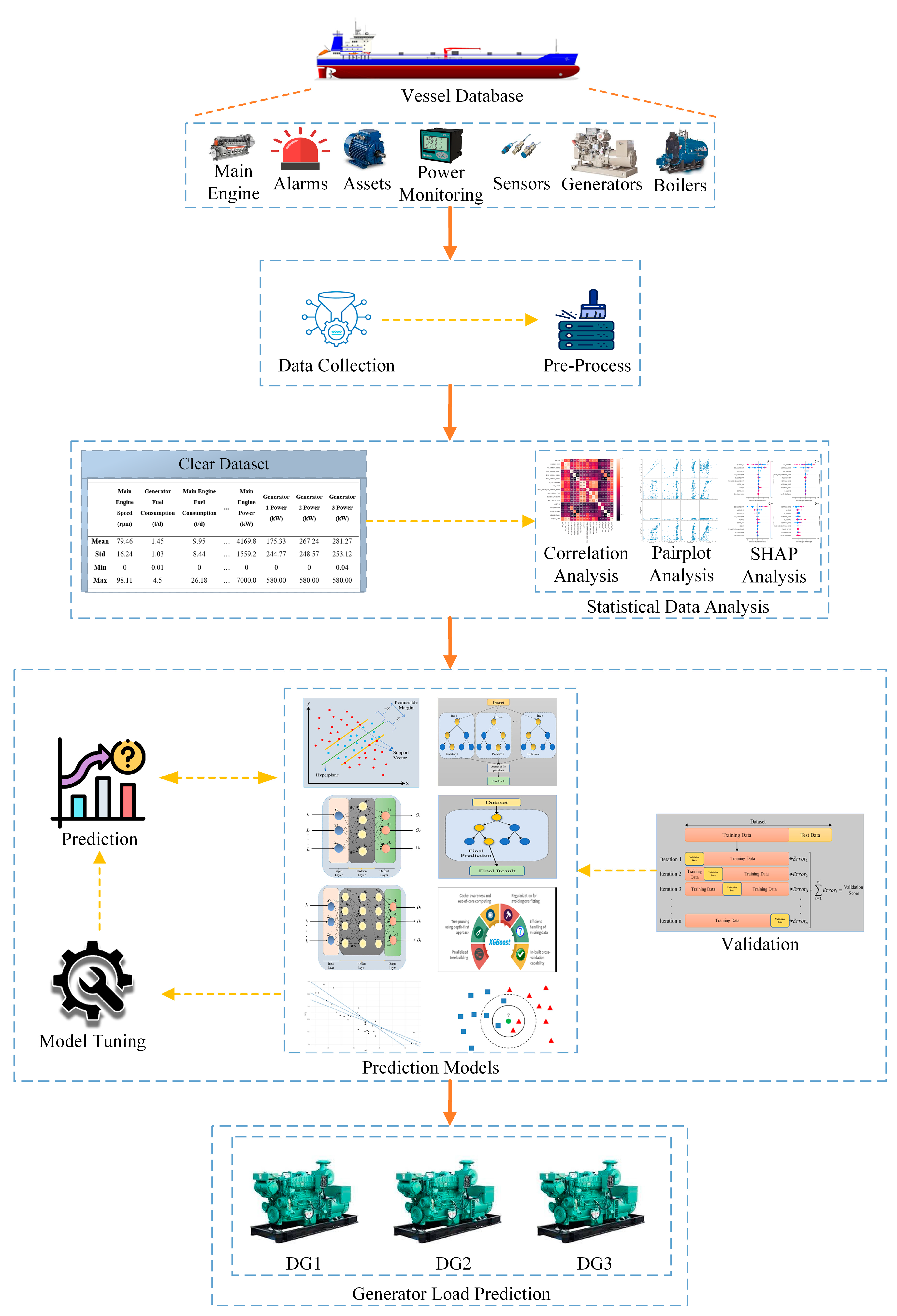
Figure 1. Methodology of the study.
Energies 16 05092 g001
Figure 2. The general structure of the investigated chemical tanker ship microgrid.
Energies 16 05092 g002
Figure 3. Pearson correlation matrix of the dataset.
Energies 16 05092 g003
Figure 4. Pair plot of the highly correlated variables.
Energies 16 05092 g004
Figure 5. Pair plot of the total load of generators and highly correlated variables.
Energies 16 05092 g005
Figure 6. Feature importance values for model output: (A) DG1 power prediction, (B) DG2 power prediction, (C) DG3 power prediction, (D) total load prediction.
Energies 16 05092 g006
Figure 7. Support vector machine.
Energies 16 05092 g007
Figure 8. A typical ANN structure.
Energies 16 05092 g008
Figure 9. A typical DNN structure.
Energies 16 05092 g009
Figure 10. Random forest algorithm structure [16].
Energies 16 05092 g010
Figure 11. Decision tree algorithm structure.
Energies 16 05092 g011
Figure 12. K-fold cross-validation.
Energies 16 05092 g012
Table 1. Vessel specifications.
ItemSpecification
Vessel TypeOil/Chemical Tanker
Gross Tonnage29,590 t
Deadweight Tonnage49,990 t
Length/Breadth183/32.3 m
Year Built2017
Average/Maximum Speed13.4/17.3 knots
Main Engine Power7000 kW
Generator Power/Count580 kW/3
Draft8 m
Table 2. Summary of the dataset.
Main Engine Speed (rpm)Generator Fuel
Consumption (t/d)
Main Engine Fuel Consumption (t/d)Main Engine Power (kW)Generator 1 Power (kW)Generator 2 Power (kW)Generator 3 Power (kW)
Mean79.461.459.954169.8175.33267.24281.27
Std16.241.038.441559.2244.77248.57253.12
Min00.0100000.04
Max98.114.526.187000.0580.00580.00580.00
Table 3. Model hyperparameters.
ModelHyperparameter
SVMNone
MLRNone
ANNsolver = ‘lbfgs’, alpha = 0.00001, max_iter = 10,000, activation = ‘tanh’, hidden_layer_sizes = (5000), power_t = 0.7, validation_fraction = 0.3, batch_size = 250
DNNinput_dim = 16, hidden_layer_count = 17, input_layer_activation_function = ‘relu’, hidden_layer_activation_function = ‘linear’, output_layer_activation_function = ‘linear’, optimizer = ‘Adam’, epochs = 1500
KNNn_neighbors = 3, weights = “distance”,algorithm = “kd_tree”, p = 20
RFn_estimators = 350, max_depth = 150
XGBNone
DtreeNone
Table 4. The prediction results for the single power diesel generator.
MAERMSEMAPE
DG1DG2DG3DG1DG2DG3DG1DG2DG3
SVR1.67361.94111.68936.37524.87037.516230.86533.81436.241
MLR1.16521.31241.18042.67013.11172.400729.59728.87731.195
ANN0.95891.00270.93241.92042.17171.891334.26524.97729.988
DNN0.57830.40250.53081.80671.49481.873331.71436.59133.773
KNN1.42941.55611.29014.41184.49084.039934.65232.79435.763
RF0.34130.22520.28920.47330.26620.471431.8798.15179.9462
XGB0.28170.14240.29260.42120.24310.509329.5476.101511.184
DTree0.23640.13060.15320.24550.20690.218217.4935.11397.7481
Table 5. The prediction results for the total power diesel generator.
Total Load Prediction
MAERMSEMAPE
SVR1.35208.323215.966
MLR1.52835.660823.302
ANN1.65756.107325.048
DNN1.08662.604914.728
KNN1.82209.631027.184
RF1.31464.948614.513
XGB1.41525.791616.805
DTree1.44529.041319.748
Table 6. 5-fold cross-validation scores (MAE) for the total load prediction.
Model
SVRMLRANNDNNKNNRFXGBDTree
Fold 11.42351.58131.74341.15171.95891.42571.47891.4925
Fold 21.43871.59751.69281.21461.98271.39521.49121.5014
Fold 31.42911.61241.71261.17381.91861.35731.46711.4874
Fold 41.44131.57311.68911.15131.89171.38411.43971.4731
Fold 51.42751.56291.69731.17251.92261.36191.45151.4667
Mean Score1.43201.58541.70701.17271.93491.38481.46561.4842
Disclaimer/Publisher’s Note: The statements, opinions and data contained in all publications are solely those of the individual author(s) and contributor(s) and not of MDPI and/or the editor(s). MDPI and/or the editor(s) disclaim responsibility for any injury to people or property resulting from any ideas, methods, instructions or products referred to in the content.