Abstract
The exponential increase in photovoltaic (PV) arrays installed globally, particularly given the intermittent nature of PV generation, has emphasized the need to accurately forecast the predicted output power of the arrays. Regardless of the length of the forecasts, the modeling of PV arrays is made difficult by their dependence on weather. Typically, the model projections are generated from datasets at one location across a couple of years. The purpose of this study was to compare the effectiveness of regression models in very short-term deterministic forecasts for spatiotemporal projections. The compiled dataset is unique given that it consists of weather and output power data of PVs located at five cities spanning 3 and 6 years in length. Gated recurrent unit (GRU) generalized the best for same-city and cross-city predictions, while long short-term memory (LSTM) and ensemble bagging had the best cross-city and same-city predictions, respectively.
1. Introduction
Problem. The usage of renewable energy sources (RES) within the energy sector has been exponentially increasing, both globally and domestically, within the 21st century. While there are several types of RES, PV arrays have seen consistent improvements in their efficiency and reductions in cost, subsequently leading to becoming more readily adopted. In 2001, only 1.5 GW of PV generation was constructed, while the global gigawatt capacity constructed in 2011 and 2021 was 65 GW and approximately 156.1GW, respectively [1,2]. Although the shift from fossil fuels to RES likely originated from the desire to decarbonize our world, the shift would not have gained much traction without the reduction in costs for these alternative sources. The estimated total selling price per peak DC watt of power generated by PV arrays across the residential, commercial, and utility sectors was projected to significantly decrease from 2010 to 2020 [3]. The prices were USD 5.71, USD 4.59, and USD 3.80 in 2010 for the residential, commercial, and utility sectors, respectively. Although these prices were forecasted to drop to USD 1.50, USD 1.25, and USD 1.00 in 2020 for the respective sectors [3], the actual prices for 2020 and 2021 were higher than initially forecasted. The prices per peak DC watt of power generated in 2020 for the residential, commercial, and utility sectors were USD 2.71, USD 1.72, and USD 1.01, respectively [4]. In 2021, the prices dropped to USD 2.65, USD 1.56, and USD 0.89 for the respective sectors.
With this trend in the reduction of the overall cost of PV arrays across all sectors, the rate of installation and construction of additional arrays would naturally increase. The projected growth of RES from 2020 to 2026 is expected to increase by more than 60% such that the total global generation is more than 4800 GW [2]. To put this in another perspective, this would amount to more than the current global generation of fossil fuels and nuclear power combined. However, unlike fossil fuels and nuclear power generation, RES are subject to variability and inconsistencies due to weather factors [1]. Therefore, there is value in applying predictive modeling algorithms to forecast PV arrays, such that grid operators can accurately predict the output power at a given instance to ensure that the load demand is met.
This predictive modeling for a given RES revolves around the weather conditions and the anticipated energy output of the system. The existing solutions of these models can be categorized by physical, statistical, or hybrid models [5]. The complexity of these models increase from physical to statistical to hybrid.
Physical models are considered the simplest of the three. Physical models describe the conversion process of solar radiation into electricity. For PV arrays, these typically include the weather conditions of solar irradiance, temperature, wind speed, humidity, and air pressure as well as the parameters of the cells within the PV itself [6]. These parameters could include the conversion process, uniformity, aging, soiling, cell temperature, and load condition [7]. Most notably, physical models do not rely on historical datasets of weather or cell conditions; instead, real-time data are utilized.
Statistic models are based on the concept of persistence, such as stochastic time series. Therefore, these models often rely on either machine or deep learning. In contrast to physical models, statistic models require a historical dataset in order to create PV projections [7]. This historical datasets are composed using time series and the associated weather conditions. Unlike physical models, the parameters of the PV cell are excluded [6]. Statistic models can employ algorithms ranging from a simple linear regressor to the more complex architecture of an artificial neural network (ANN). Stochastic models are most prevalent in literature regarding PV power projections. The dependence on historical data is considered a shortcoming of stochastic models, and this dependence is reduced in hybrid models.
While hybrid models are any combination of the two aforementioned classifications. The objective of the hybrid model is to mitigate the shortcomings of the different constituent models [5]. Therefore, these tend to be the most accurate yet complex models.
Our Contributions. This study compares the accuracy of projections from 15 algorithms on expansive spatiotemporal datasets. These algorithms were classified as statistic models because they strictly used historical time series data. Within that classification exists both machine learning and deep learning algorithms. The machine learning models analyzed in this study were k-nearest neighbors (KNN), linear regression, linear stochastic gradient descent regression (LSGDR), elastic net, partial least squares (PLS), ridge, kernel ridge, SVR, NuSVR, decision tree, random forest, and ensemble bagging. Meanwhile, the neural networks used were MLP, LSTM, and GRU. Although LSTM has been widely tested in prior works and GRU has been compared but less frequently, it is the contrasting of the two models within this study that brings forth the unique contribution. The datasets used in this study included five locations, where all but one of the locations had 6 years of data. The accuracy of the projections was compared for both same city and cross city. In this study, it was found that GRU generalized the best for same-city and cross-city predictions, while LSTM and ensemble bagging had the best cross-city and same-city predictions, respectively.
Significance. Given the inconsistencies inherent in RES due to their reliance on weather and external factors, a diverse collection of RES and predictive modeling of these respective sources is necessary to maintain the load demand of electric grids. While all RES must receive careful consideration in terms of potential installation locations, for PV arrays, the impacts of partial shading and typical weather patterns of the region are critically important [8]. That said, PV generation is most closely tied to cloud cover [9]. When there are no clouds, PV generation follows a diurnal curve as the sun traverses the sky, which is both smooth and predictable.
However, when clouds are present, they impact both the quality and quantity of the output power generated [9]. One such example is when there are sparse cumulus clouds in an otherwise relatively clear day [9]. Due to the sparsity of these clouds, the shading upon the given PV array is inconsistent. Therefore, the quality of the output power is greatly diminished, while the quantity remains relatively high. This contrasts with when there are opaque stratus clouds that linger for hours, thereby causing the output power to be greatly diminished, while the quality remains high [10]. Whether a cloud is drifting such that it is just shading an array or that it is just departing, the abrupt nature of this change creates a step change that is either a decrease or increase in the power generation [11]. This is classified as ramping and is a factor that grid operators must consider when balancing load demands.
Any significant surplus or deficit of PV power generation, if multiple sources are tied together, must be balanced with an equal but opposite allocation such that the load demand of a given region is met [9]. The power quality from a PV array can be most easily visualized on the consumer end when voltage flicker occurs. While low power quality is not directly indicative of voltage flicker occurring, it would occur more frequently given increased variations in the quality of power delivered. Voltage flicker is when the demand for electricity momentarily rises above the threshold of power generation that can be delivered [12]. This can most easily be observed in the brief flickering of lights after a large appliance was activated. That said, preventing voltage flicker and moderating ramping effects are just a few of many parameters that govern the output power generated by a singular or collection of PV arrays. These are just a few tasks that are categorized as electric grid management, as shown in Figure 1. Therefore, the more accurate the projections of output power from RES, the more efficient and cost-effective energy management can be. The grid operators would be able to either pull from energy storage units to meet the grid’s load demand or allocate any surplus of energy generated to these battery units. Additionally, with a better understanding of the amount of energy generated by a source at any given point, the grid operator would be able to better transmit the energy to regions with greater demand. The impact of clouds upon PV arrays influences the amount of solar irradiance that is received by the arrays. This irradiance can be subcategorized based on the angle and method that it hits each panel of the PV array. These distinctions include the diffused horizontal irradiance (DHI), diffused normal irradiance (DNI), global horizontal irradiance (GHI), and the corresponding clear sky variations. Although the different distinctions of irradiance are grouped as one in Figure 1, it also becomes evident that there are multiple other parameters that influence the output power of PV arrays. These include but are not limited to the cloud type and amount of cloud cover, wind speed, relative humidity, temperature, and other weather parameters. Therefore, given these characteristics and the additional complexity of the conditions governing the power generation of PV arrays, logically, these arrays would greatly benefit from the usage of predictive modeling. The output power can be modeled given the weather conditions at the location. These forecasts are best accomplished using machine learning.
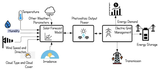
Figure 1.
The connection between inputting weather data into a model and utilizing that model in assisting in the management of the electrical grid. Source [13].
Artificial intelligence is the parent category that contains machine learning, and within it exists a subset called deep learning. Machine learning can be considered a shallow neural network, as it allows programs to learn from data without being declaratively programmed [14]. Deep learning differs by having several hidden layers, complex connectivity architectures, and different transfer operations [14]. Deep learning algorithms are synonymous with neural networks. The term machine learning was first used in 1959 by the American scientist Arthur Lee Samuel to describe the field of computers that enables computers to learn from data without being directly programmed [14]. However, in the contemporary era, machine learning has become universal. Its usage has entered the everyday workspace, household devices, automobiles, and any sphere with the intention of providing ease of life to people. From the ubiquitous growth of machine learning, it has also been employed to generate predictive models for the output power of PV arrays.
PV Prediction in Literature
Related Works. As stated, prior art in PV predictions can be classified into physical, statistical, or hybrid models. Statistical models are most commonly employed within these publications. These publications compare different machine learning and deep learning models against one another. In most cases, there are only a handful of models whose performances are compared, while there are a few publications that are more comprehensive, comparing the results across articles. When using stochastic models on PVs, there are more types of machine learning algorithms applied to PV projections than those of deep learning. Typically, the machine learning algorithms of linear regression, ridge, lasso, elastic net, decision trees, random forests, random-forest-based ensemble bagging, and support vector machines are applied [14]. In one particular study, an ensemble method that was developed was composed of the elastic net, gradient boosting, and random forest algorithms.
However, before determining which model is best to use, one must first understand the different durations of forecasts and their corresponding applications. Power generation forecasts are typically categorized into four groups based on the length of the projection: very short-, short-, medium-, and long-term forecasts [15]. Intraday forecasts are classified as very short-term, and for these projections, onsite measurements are necessary. These very short-term forecasts are applied in real-time operations, such as spot markets, power smoothening, real-time power dispatching, and automatic generation control [15]. Short-term forecasts are typically between 1 h to 1 week ahead. These projections are typically utilized for reserve optimization, economic dispatching, transmission scheduling, unit commitment, storage system management, and day-ahead markets [15]. Medium-term forecasts typically range from 1 month to 1 year [1], while long-term forecasts tend to range from 1 to 10 years [15]. These forecasts are mainly applied to the power sector for determining scheduling and planning within the sector.
In statistical modeling, deep learning algorithms are tested as frequently as machine learning algorithms. These algorithms consist of multiple layers, each layer composed of multiple nodes, thereby garnering the name neural networks. These layers are the input layer, the hidden layer, and the output layer. While not necessary, the hidden layer can be a single layer or multiple layers. Additionally, the output layer may consist of a singular or a multitude of nodes, depending on how many dependent variables are desired. The most overarching type of neural network is the recurrent neural network (RNN). The standard deep learning models used within existing studies include multi-layer perceptron (MLP), LSTM, grated recurrent unit (GRU), or convolutional neural network (CNN) [16]. LSTM models and other RNNs have also been used for these predictions because of the strength of their time series ability.
Regardless of the type of neural network used, the algorithms typically outperform machine learning models. In one study, a joint Siamese CNN and LSTM model (SCNN-LSTM) was developed [16]. This model was then tested against an MLP, LSTM, and 3D-CNN. The SCNN-LSTM outperformed the 3D-CNN, which outperformed the LSTM and MLP, respectively, for 10 min ahead forecasts. The better performance of the SCNN-LSTM and the 3D-CNN could be attributed to the ability of deep learning models to handle images and numerical data. In another study, a Bayesian neural network was tested against an SVR and a regression tree [15]. These models were tested under conditions where minimal input features were provided to determine the day-ahead forecasts. Within this study, the three models were trained and tested on the same dataset for optimal comparison analysis. The results were that the Bayesian neural network significantly outperformed the SVR, which moderately outperformed the regression tree. Another study compared 24 machine learning models for deterministic day-ahead forecasts using a 2-year-long dataset at 15 min resolution [15]. From this comprehensive comparison, it was found that a neural network composed of an MLP had the best overall performance, followed by SVMs.
To properly compare the accuracy of different models, error analyses and accuracy evaluations must be conducted. Under different sky conditions, the accuracy of a model, let alone the baseline, will vary. The California Renewable Energy Collaborative demonstrated that a %RMSE value up to 6% could be expected when forecasting a day ahead under clear sky conditions [17]. Meanwhile, under nonclear sky conditions, %RMSE values of at least 20% with a few outliers ranging between 40% and 80% were observed [17]. A study that focused on a type of ANN determined that this type of algorithm could achieve %RMSE values within the range of 15.2–16.3% for the day-ahead forecasts [18]. Additionally, the forecasting techniques of ANNs on average have been proven to be considerably effective given the inherent ability to record nonlinear abrupt changes that are caused by rapid changes in the environmental conditions of the relationship between the input and outputs [15,18].
Similar Works. While there are no prior works that align completely, for select aspects, there are a few that are more closely related. There are few studies that incorporate data from two or more locations. Based on the data compilation in one study, annual and quarterly projections were generated for two locations, one in China and another in the United States [19]. The dataset utilized was sampled quarterly, and the forecasts were made annually, for an undisclosed length of time and location. The study shares similarity only in the usage of datasets from more than one location. Another study shares similarity by utilizing data from multiple locations and employs a rolling window [20]. The study compiled 14 months of data from 7 wind farms, 10 PV arrays, and the respective weather data from NREL collected in Oahu, Hawaii. Although this study utilized data from multiple locations, it was used by locations in close proximity. This was done such that by knowing the distance to the nearby location with a given weather event, and the speed that the weather event was moving at, the arrival of the observed weather event could be anticipated at the original site. In contrast to what is proposed in this manuscript, the models compared in both of these similar studies were not trained on the data from one dataset and tested on another. Instead, the models were trained and tested on data from the same location. Although no studies were found where cross-city projections occurred, comparable to this study, a simple LSTM structure was used in [21]. The baseline structure of an LSTM without supplemental deep learning networks was attached.
Prior Datasets. As relevant as it is to understand differences between different applications of statistical algorithms and the forecasting windows applied to PV generation, the parameters used also have different predictive capabilities. The parameters of GHI, wind speed forecasts, and ambient temperature are considered basic because they are most used [22]. While the GHI from the actual, hourly, and daily mean GHI ambient temperature shifted by 1 h, azimuth, declination angles, and elevation are the most effective at predictive capability. However, these are considered complex as these are calculated from the basic inputs without requiring additional data [22]. Meanwhile, the daily mean GHI, supplemented by declination angle, azimuth, and modeled 15 min elevation, are useful if operating at a low budget [22]. They come at the cost of a reduced resolution of generated forecasts. In short, the most used predictors for the output power are the average GHI, temperature, wind speed and direction, precipitation, humidity, and cloud cover.
Across two comparative analyses spanning 31 studies, there are significant variations in the sampling rates, lengths of datasets, and locations tested within each study. The average sampling rate was split equally between 15 and 30 min intervals. There were sampling rates as frequent as once per minute and as infrequent as once an hour [14]. The length of each dataset varied from less than a year to the rare few with 5 years of data. However, the average length of data available was between 1 and 2 years, erring on 2 years [22]. Furthermore, all but 2 of the 31 studies had datasets that were restricted to one location. These 2 studies that serve as outliers are first referenced in the similar work section.
2. Materials and Methods
2.1. Spatiotemporal Weather and PV Power Data
In this subsection, the compiled weather and PV dataset is introduced, as well as the real-world applications of the dataset. The weather data were obtained from the National Renewable Energy Laboratory (NREL) [23], while the output power of the PV arrays was obtained from the Special Interest Groups Energy (SIG Energy) of California and the University of Massachusetts Amherst [24]. For each of these sources, the usage rights are only restrictive against commercial usage.
2.1.1. Dataset Analysis
The empirical data for this study were compiled from three different databases. The dataset consists of the weather data and the output power of a given PV array, taken at uniform intervals of date and time. To maintain standardization across the dimensions of the dataset, the weather data from each of the five locations were obtained from NREL [25]. The weather data from NREL are available from the years 1998 to 2021, and they are sampled at a 30 min refresh rate with a localized region of 4 km [23]. The initial city was Amherst, MA, wherein the power data were obtained from the 155 kW capacity PV array atop the Computer Science Building at the University of Massachusetts Amherst [26]. The locations of the other PVs were in the Californian cities of Davis, Huron, Santa Barbara, and La Jolla with output power capacities of 143.2, 53.8, 42.5, and 41.7 kW, respectively [27].
Given the vast distances between some of the chosen cities, it is necessary to provide the rationale behind the selection. The city of Amherst, MA, was initially selected to serve as a ground truth for the weather and PV power data collected by an undergraduate capstone project at WPI given the relative proximity of the cities. In this capstone, an array of irradiance sensors were utilized to predict the output power of a small PV array. Given that the initial plan was to train the model on the data from Amherst and to test it on the data collected by the irradiance sensors, a sampling window from 10 a.m. to 3 p.m. with a 30 min refresh rate was proposed. This was deemed an acceptable window given the setup and management of the undergraduates. The direction of this research changed, and with it, the number and the scope of the cities included. This enabled cross-city projections, where a given algorithm model was trained on data from one city and tested on another. In order to avoid the persistence of weather in a localized region, it was necessary to locate additional PV arrays outside of New England with a comparable sampling frequency and length of data available. The cities in California were selected based on these criteria. Additionally, the capacities of the PV arrays were large enough that comparisons could be made. The city of Davis in California was selected as it had a PV array nearly equal in size to that of Amherst and was located on a similar latitude. The remaining cities in California were selected based on the subsequently decreasing capacities of the PV arrays located at the given cities.
Although multiple years of data were obtained from each source and location, unfortunately, there was no overlap of years between the site in Massachusetts and those in California. The University of Massachusetts Amherst accrued historical data of the power output of their array with a 15 min refresh rate from the years 2017 up until the current day when this was written. The output power from Amherst was compiled from the year 2018 to 2020. This contrasts with the years available from SIG Energy. Although the data also contained a 15 min sampling frequency, they were only available from 2011 to 2016. For each year of data available, the dataset followed the calendar year by starting on January 1 and ending on December 31. Fortunately, despite this discrepancy, the weather data maintained a consistent dimension of parameters for each location. When conducting cross-city analyses on 3 years of data, all five cities were used. Therefore, only the cities in California were used when conducting cross-city projections for 6 years. To reduce any potential differences that may arise when comparing the datasets from California and Massachusetts, only the last 3 years of the SIG Energy data were utilized for the cross-city analyses across the five cities.
The datasets underwent preliminary preprocessing, prior to any standard preprocessing required for the algorithms. This preliminary preprocessing predominantly consisted of filtering the dataset to match the daily window of 10 a.m. to 3 p.m., composed of 11 data points per day. However, in addition to that, the output power from SIG Energy was converted from kWh every 15 min to kW per 30 min window. The datasets for each city are composed of 22 columns, wherein the first 5 are the date and time, the next 16 are weather data, and the last column is the output power. For the datasets of 3 years in length, there are 12,056 rows of data, while the datasets of 6 years in length are twice that at 24,112 rows. The columns and the respective units are described in more detail in the bulleted list.
2.1.2. Data Description
- Year: For the data at Amherst, the years range from 2018 to 2020, while the Californian cities range from 2011 to 2016. Only the last 3 years from the Californian cities were compared with those from Amherst.
- Month: All 12 months of data are included for each year of data available.
- Day: Each day, including leap days, was included.
- Hour: Only the hours from 10 a.m. to 3 p.m. and subsequent data points within were used.
- Minute: The data were sampled at a 30 min sampling frequency.
- Diffused horizontal irradiance (DHI) (W/m): The solar radiation that has indirectly arrived at a given location after having been scattered by the clouds and other particulate matter in the atmosphere. The solar radiation arrives equally from all directions [28].
- Diffused normal irradiance (DNI) (W/m): It is representative of the total radiation that arrives perpendicular to a given surface, and is measured by photoelectric detectors [23].
- Global horizontal irradiance (GHI) (W/m): It is representative of the total amount of shortwave radiation that is received from the sun by a given horizontal surface. The GHI was measured by thermoelectric detectors and can also be calculated from the equation .
- Clear sky (DHI) (W/m): Clear sky denotes the conditions where there is an absence of clouds across the entire visible sky. The clear sky DHI is therefore the upper threshold that the DHI could achieve.
- Clear sky (DNI) (W/m): The clear sky conditions for DNI.
- Clear sky (GHI) (W/m): The clear sky conditions for GHI.
- Cloud type (unitless): NREL classifies clouds into 11 types. In increasing numbers, these types are probably clear, fog, water, supercooled water, mixed, opaque ice, cirrus, overlapping, overshooting, unknown, and dust. Therefore, this specific column contains discretized data rather than continuous.
- Dew point (C): The temperature at which water vapor can condense. At the dew point, a saturation of water vapor is reached; therefore, fog, clouds, and precipitation may develop [29].
- Solar zenith angle (degrees): The angle is the angle that the sun is relative to an axis that is normal to a surface [30]. This angle decreases as midday approaches, reaches a minimum value, and then increases afterward. It equals the latitude minus the angle of solar declination.
- Surface albedo (degrees): The fraction of solar radiation that is reflected by the surface of the Earth [31]. This value varies between zero and one, whereby a higher value indicates a larger amount of radiation that was reflected off the Earth.
- Wind speed (m/s): The speed of the wind within the atmosphere. This measurement was taken at the surface and scaled to within the atmosphere [23].
- Precipitable water (mm): The cumulative amount of water vapor contained within a vertical column of a given space of the atmosphere. The volume of water vapor is typically expressed as if it had condensed.
- Wind direction (degrees): The direction is determined by the nearest hourly values of the second iteration of the Modern Era Retrospective Analysis and Research Applications [23].
- Relative humidity (%): The total amount of water vapor in the air compared with the maximum vapor that the air can retain at a given temperature [29].
- Temperature (C): The temperature is measured at the surface level but scaled to be the temperature within the atmosphere by a factor of 6 °C/km of elevation increased.
- Pressure (mbar): The measured pressure of the atmosphere.
- Output power (kW): The power generated by the PV array. The upper threshold of this value is dependent on the size of the array, while the instantaneous value is dependent on the weather factors above.
2.2. Machine Learning Methods
In this section, the techniques and algorithms covered within the paper are introduced and discussed. The statistical models covered are KNN, linear regression, LSGDR, elastic net, PLS, ridge, kernel ridge, SVR, NuSVR, decision tree, random forest, ensemble bagging, MLP, LSTM, and GRU. Since the dataset used in this research is time sequencing, it dictates that the regression variations of the models should be used instead of classification.
K-Nearest Neighbors. The KNN algorithm utilizes a type of instance-based learning based on the differences between features. The algorithm uses the distance function to determine a set of samples, whose length is dictated by the value of k, that are closest to the target variable [32]. The algorithm stores the entire training dataset during the training phase. The algorithm then creates a set of instances of length k that most closely maps to the target. The prediction of the model is created based on the similarity that new observations have with the aforementioned set formed during training. These new instances are compared with each instance within the training set; the prediction is derived from the average of the response variable. In regression-based KNN, the response variable is the mean of the output variable [32]. In greater detail, the KNN algorithm computes the prediction Y for each instance of x by averaging the targets from the nearest k instances from the set, as described in Equation (1):
where, in this simplified example, represents the training examples, and is the set of nearest points [32]. It can be difficult to determine the optimal value of k as there is an inverse relationship between k and the error on the training set but a direct relationship with the error on the test set. The distance function, used to calculate the Euclidean distance d between the variables x and y, is used in the KNN algorithm as described in Equation (2).
Linear Regression. This algorithm is one of the simplest models that could be tried when conducting regression on a dataset. As shown in Equation (3), the correlation between the independent variable X and the dependent variable Y is bridged with a coefficient for each dependent variable and an intercept [33]. However, as the complexity of a dataset increases, the likelihood of linear regression producing accurate projections likely decreases. However, it is still beneficial to include the model to serve as a baseline:
where y is the output or dependent variable, are the independent features, are the coefficients of the linear model, and is the intercept term.
Linear Stochastic Gradient Descent Regressor. A linear regression model that uses stochastic gradient descent as an optimizer. This model iteratively updates the model weights using a small, randomized subset of the training data instead of the entire dataset, therefore making it computationally efficient for larger datasets [34]. The linear function that is used to predict the target variable is described in Equation (3). The objective of this regressor is to determine the values of w and such that the loss function is minimized. Additionally, the loss function must be defined within the predicted and actual values of the target variable [34]. In this case, the loss function is the squared error, and the penalty function is the elastic net.
Partial Least Squares. PLS is an efficient regression model, based on covariance, that is often used in circumstances where there are many independent variables. In particular, PLS is often used when the independent variables are correlated. PLS reduces the number of variables to predict a smaller set of predictors [35]. This smaller set is then used to perform the regression analysis. Although there are two types of PLS for regression, PLS 1 and PLS 2, the difference between them is if there are one or multiple dependent variables, respectively. Given that there was only one dependent variable in this research, PLS 1 was used [35]. The formula for PLS regression is described in Equation (4):
where Y is the matrix of dependent variables, X the matrix of independent variables, and B the matrix of regression coefficients generated by PLS of Y on X with h number of components. Meanwhile, , , , , and are matrices generated by the algorithm, and is the residual from the algorithm.
Ridge Regression. Ridge regression is an algorithm that estimates the coefficients of multiple regression models where the independent variables are highly correlated. The ability of ridge regression to handle this multicollinearity separates it from partial least squares regression. As a result, the ridge is most used in applications where there are many independent variables. Typically, when using ridge regression, it can be assumed that the independent and the dependent variables have been centered [36]. In ridge regression, regularization is used, such that the penalized sum of squares is minimized to yield the ridge coefficient.
Kernel Ridge. Kernel ridge combines the linear least squares and -norm of ridge regression with the kernel trick. Therefore, a linear function is learned in the space induced by the respective kernel and data [37]. However, in this study, this model uses a polynomial-based kernel function; therefore, a nonlinear function is mapped to the original space. Within this research, the polynomial kernel function has a degree of 10. The resulting kernel ridge regression model differs from SVR from the loss function that is used [37]. For kernel ridge, squared error loss is used, while epsilon-insensitive loss is typically used by SVR.
Elastic Net. Elastic net is a sparse learning regressor that solves the limitations of lasso and ridge regression, yet also maintains both as special cases. It uses a weighted combination of the - and -norm, where these regularization methods are used by lasso and ridge, respectively [38]. In lasso regression, the independent variables are shrunk to a central value. Elastic net is able to generate reduced models by creating zero-valued coefficients [39]. The algorithm is often preferred, as it is able to apply the optimal regularization technique based on the nature of the data. As a result, the elastic net is considered to be a parent model to lasso and ridge regression [38]. Elastic net is described further in Equation (5):
where N is the number of observations, is the response at observation i, is the data as a vector of p values at observation i, is a positive regularization parameter, is the penalty term, is a scalar that ranges between zero and one, and and are scalars [39]. When equals one, then the elastic net applies the -norm and functions like lasso regression; alternatively, as approaches zero, the elastic net approaches the -norm, therefore functioning comparable to ridge regression. If the elastic net is operating similarly to ridge regression, then the algorithm would use gradient descent to generate the projections. If the elastic net is either completely or partially configured to operate as lasso regression, then subgradient descent or coordinate descent would be used. In the case where is between zero and one, then both the - and -norm would be used by the algorithm.
Decision Tree. Tree-based regression models benefit from a simpler structure and efficiency, in regard to the large domains of datasets. This is a result of the fast divide-and-conquer behavior of the model, based on the greedy algorithm wherein the larger dataset is split recursively into smaller partitions [40]. These tree-based algorithms are effective for large datasets yet prove to have shortcomings, such as instability on smaller datasets. This instability could arise from a small change during the training phase, leading to different nodes being created, causing the said instability and inconsistent results. A decision tree is composed of the potential decisions and corresponding repercussions, constructed in a flowchart-like tree structure [32]. The outcome of a node is represented by the branches or edges. Each node has either a decision node, chance node, or end node. A boolean argument is representative of the branches or edges, and the decision tree weighs the three aforementioned conditions.
Random Forest. Random forest is a type of supervised learning algorithm that effectively uses ensemble bagging to tackle regression- or classification-based problems. During the training phase, the algorithm creates multiple decision trees and then outputs the mean prediction of the trees [41]. The benefit of having multiple trees, instead of just one, is that the collection of trees protects against the errors of the individual counterparts. The random forest model acts as an aggregator to the mean projections of the total decision trees constructed. In this study, both the random forest and the decision tree algorithms use squared error as the loss function.
Ensemble Bagging. The basic principle behind ensemble methods is to create an integrated group of baseline models, typically considered weak learners, into a more robust model [14]. The more robust a model is, the more capable it is to adapt to changes in the dataset, thereby providing more accurate and reliable performances regarding the projections. There are three types of ensemble methods that are typically used: bagging, boosting, and stacking. In this study, a version of ensemble bagging that is composed of random forest models is utilized. Bagging, whose name was derived from bootstrap aggregation, is where multiple baseline models are trained in parallel on portioned subsets of the training data. During the training phase, bootstrapping occurs, where the original dataset is randomly sampled with replacement. Sampling with replacement means that every time a sample is collected by a model, it is then replaced [42]. This ensures that each round of sampling is independent and does not interfere with the next round. Then, the final prediction of the algorithm is obtained from a voting aggregation of the final predictions of the baseline models [14]. Given that random sampling with replacement is used within ensemble methods, instead of altering the biases of the models, the variance of the projections is reduced.
Support Vector Regression. Support vector regression is an abstracted version of support vector machines. SVRs are better suited for times-series predictions, which are the condition that governs forecasts for PV power generation when using irradiance. In a more general sense, the SVR is derived from a function that maps the input patterns to those of the output. This is done based on a given set of training data that aim to minimize error by individualizing the hyperparameters. The input features are mapped using a nonlinear mapping process to a high-dimensional space [15]. The nature of the SVR is described in Equation (6):
where is the training set and many of the ’s are equal to zero. However, there are some limitations to the SVR algorithm: it lacks probabilistic interpretation, there is difficulty in selecting the optimal regularization parameter C, and the algorithm is restricted to using positive semidefinite kernels [43].
The projections of NuSVR are also compared in this study. Nu is a parameter used to control the number of support vectors and replaces the parameter epsilon in epsilon-SVR [44]. In this case, an nu value of 0.35 was used. For both SVR and NuSVR, the radial basis function kernel was used as the activation function.
Multilayer Perceptron. MLP is a type of feed-forward supervised learning algorithm. It is composed of three layers, an input layer, a hidden layer, and an output layer. Each layer is multidimensional and can handle nonlinear calculations. However, in the case of this study, the output just has one dimension. Each neuron in the hidden layer transforms the previous dimensions of the input layer using a weighted linear summation, then utilizes a nonlinear activation function [45]. Additionally, backpropagation is used without the need for an activation function in the output layer, effectively using the identity function as an activation function. In this study, for forward propagation, the rectified linear unit activation function is used. Additionally, the Adam optimizer, an extended version of stochastic gradient descent, and the square error loss function are implemented into the MLP. The MLP algorithm is beneficial as it has the capability to learn nonlinear models and learning models in real time. However, the hidden layers have a nonconvex loss function, which leads to the potential for multiple minima to exist [45]. Therefore, any differences in the random weighting of the initialization can cause differences in the accuracy of the validation. Additionally, the MLP is subject to sensitivity when feature scaling.
Long Short-Term Memory. LSTM networks are composed of a few types of gates that contain information about the previous state. The information of the LSTM is either written, stored, read, or eliminated in the cells that serve as a memory stage for the model [21]. The four potential processes are accomplished through the opening or closing of the gates. The cells act on signals they receive, and based on the strength of the signal, they will either transmit or block information. The LSTM model is composed of three different states, the input, hidden, and output state. Within each unit of the LSTM, there exist a cell state, ; an input gate, ; an output gate, ; and a forget gate, , displayed in Figure 2. The forget gate is tasked with determining which information is kept or eliminated from the cell state [21]. This decision is determined by the logistic function , as described in Equation (7). This function will either output a value of zero, to keep the information, or a value of one, to forget it:
where, in Equations (7) and (8), is the activation function, is the weight of the forget gate, is the bias of the forget gate, is the input at time t, is the hidden layer at time , is the weight of the cell, and is the bias of the cell. The input gate, forget gate, cell state, and output gate are shown in Figure 2, the LSTM cell. The input gate, , and the cell state, , are described in Equation (8). The input gate determines which input values are updated by the blocks of the LSTM.
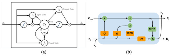
Figure 2.
The LSTM unit with the forget, input, and output gates: (a) the LSTM unit, source [21], (b) the LSTM cell.
The output state determines which segment of the cell state is permitted to output. The formula for the output state, as described in Equation (9), includes a tanh and is multiplied by another logistic function whose output is scaled similarly to the forget state:
where is the activation function, is the weight of the output gate, and is the bias of the output gate. The input data to the LSTM are composed of a three-dimensional array. The first dimension is represented by the number of samples in the network, the second dimension is the time steps, and the third is the number of features in one input sequence [21]. In order for the LSTM to properly handle the dataset, a sliding window was created such that data could be inputted into the algorithm. The sliding window is discussed in greater detail in the preprocessing section. That said, the resulting size of the three-dimensional array inputted into the LSTM was 11 by 3 by 20. The version of the LSTM in this study contains a batch size of 64, a hidden size of 64, three dropout layers, and an MSE loss function used given the regression nature of the dataset. Additionally, the Adadelta optimizer was determined to yield the best performance by trial and error. The Adadelta optimizer is a more robust version of the Adagrad optimizer. Adadelta adapts the learning rates based on a moving window of gradient updates; therefore, it is not necessary to set an initial learning rate [46].
Gated Recurrent Unit. The GRU is a type of RNN and was introduced in 2014. It was implemented to solve the issue of the vanishing gradient that is a problem within standard RNNs [47]. Similar to the LSTM, the GRU is able to handle sequential data, such as time series, speech, and text. Similar to the functionality of the LSTM, the GRU uses gating mechanisms to selectively update the hidden state, subsequently updating the output layer. In particular, the GRU has an update gate and a reset gate that compose the gating mechanisms. However, unlike the LSTM, the GRU does not contain an internal cell state. In the GRU model, the reset gate determines how much of the previous information of the hidden state should be forgotten. The reset gate of the GRU is analogous to the input and forget gate of the LSTM [48]. Meanwhile, the update gate determines how much of the previous information should update the hidden state, and subsequently be passed into future units of the algorithm. The update gate is comparable to the output gate within the LSTM. The current memory gate is a subset of the reset gate. This gate introduces nonlinearity to the input data. Another benefit of the current memory gate being a subset of the reset gate is that it is able to reduce the impact that the previous information has on the current information that will be transmitted to any future units [48]. The final output of the GRU model is calculated based on the hidden state and is described in Equation (10):
where is the reset gate, is the update gate, is the candidate hidden state, is the hidden state, is the prior hidden state, and are the learnable weight matrices, and is the input at time step t. The sigmoid function is applied to scale the result between zero and one. The GRU model is able to solve the vanishing gradient by storing the relevant information from one time step to the next of the network [47]. The GRU used in this research shared the dimensionality of data inputted as the LSTM because the same sliding window was employed. Additionally, the model utilized an averaged stochastic gradient descent optimizer with an MSE loss function.
2.3. Preprocessing
The research that was conducted included machine learning and deep learning models. To improve the accuracy of the projections of these models, feature selection was conducted on the dataset. The parameters of interest were determined from the generation of Kendall correlation heatmaps. Additional preliminary testing was conducted to evaluate the optimal normalization technique to be used on the compiled dataset. The normalization methods that were compared were min–max, z-score, and decimal scaling. These methods were evaluated based on the accuracy of the models given same-city and cross-city projections when trained at Huron. Ultimately, min–max scaling was used for the evaluations within the study. The data were then either split sequentially or randomly depending on the type of model used, although in both cases, there was a 70/30 split of training data to testing data. Sequential data were used for the deep learning models of the LSTM and GRU, while all the other models underwent random sampling. The machine learning models were inherited from the scikit-learn library. Based on the input requirements for the machine learning models, the entire training dataset was inputted in one instance prior to testing. This is in contrast to LSTM and GRU algorithms. The two deep-learning models were trained and tested using a sliding window. The sliding window dropped the year but retained the other independent parameters of data and was composed of 11 rows such that the equivalent of 1 day of data was used in each instance. The output power data from the 11th row were the dependent variable tied to the entire sliding window. The sliding window and the respective output power value were saved as a pickle file. The hyperparameters of each model were tuned through trial and error.
The experimentation remained the same for each model. The models were trained on the dataset from one city, then tested three times on the dataset of a given city. The location of the testing city was cycled after recording the results of the evaluation metrics from the mean and standard deviation of each iteration. The process was then repeated by cycling through which city was used as the training dataset. The same-city projection and cross-city projection results, from datasets of a given length of years, were extracted from the large matrix of results generated.
The above process was conducted for the five cities with datasets of 3 years in length and then repeated for the four cities with 6 years of data. Varying the length of years of data inserted into the models allowed for deeper evaluations of the performances, namely, to observe if there was any fall-off of accuracy for certain models.
3. Results
3.1. Evaluation Metrics
Although there is no standardized evaluation metric applied to determine the accuracy of forecasts for the output power of PVs, there are a few that are more commonly used. The acceptance of using MSE or RMSE varies from one report to another, as there are numerous metrics used within each study. Occasionally, is used as well. is a statistical measurement of how well the regression coefficient matches the ground truth. For scores, the closer a score is to one, the more accurate is that projection, while smaller decimals and negatives are indicative of increasing inaccuracies. This is in contrast to the ideal MSE and RMSE values, where the more accurate the projection of a model is, the closer the value would be to zero. The results from MSE and RMSE are strictly positive.
At least in regard to electricity forecasting, RMSE appears to be a popular evaluation metric [49]. The three accuracy measurements of , MSE, RMSE were used to better enable comparisons with prior contributions. The evaluation metrics used are described in Equation (11):
where n is the number of iterations, is the observed value, and is the predicted value.
3.2. Analysis
In any dataset, particularly in datasets with many dimensions, it is beneficial to conduct feature selection. Feature selection is a technique employed to improve the accuracy of projections by removing the multicollinearity in independent variables. Multicollinearity between two variables can be easily identified when the magnitude of the correlation coefficient is equal to or exceeds 0.7 [50]. This is shown in Figure 3, where a cross-correlation heatmap was generated based on the Kendall coefficient. The Kendall correlation was selected as it is both more robust and ideal for time series data because it can handle normally and non-normally distributed data.
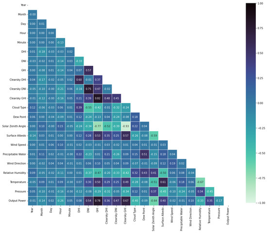
Figure 3.
The Kendall cross-correlation of the parameters of the dataset.
When interpreting heatmaps, the learned weight that a given parameter on the horizontal axis has on a parameter on the vertical axis is given by the value at the point of intersection of the two parameters. If the value of the coefficient is greater than zero, there is a positive relationship between the two parameters, while if the coefficient is less than zero, then there is an inverse relationship between the parameters. Additionally, if the coefficient is equal to zero, then there is no correlation.
Although there is a slight variation in the value of the weight coefficients, based on the city used in the cross-correlation, the relative ratios between the weights remain similar. There are a few cases of multicollinearity within Figure 3. This occurs between GHI and clear sky GHI, DNI and clear sky DNI, GHI and solar zenith angle, and clear sky GHI and solar zenith angle, with coefficient weights of 0.82, 0.75, −0.77, −0.93, respectively. According to the heatmap, the parameters with the greatest correlation with the output power of a PV array are GHI, followed by clear sky GHI, solar zenith angle, and DNI, with weights of 0.78, 0.67, −0.64, and 0.54, respectively. Unfortunately, the select variables that are highly correlated with the output power also exhibit multicollinearity with the other correlated predictor variables. To remove the multicollinearity within the dataset, the dimensions of solar zenith angle, clear sky DHI, clear sky DNI, and clear sky GHI were removed. However, the accuracy of the model projections decreased relative to before the dimensionality of the dataset was reduced. Therefore, the complete dataset was used for the remainder of the comparative analyses. Prior to the reduced dimensionality, the parameters that were highly correlated with the output power of PVs align with that of prior art. Logically, the more solar radiation that a given area receives as measured by GHI, the greater the power output of the array is. The reason the weight coefficient for the solar zenith angle is negative is that as the sun rises in the sky, its angle from an axis normal to the ground decreases, indicative of an inverse relationship between solar zenith angle and output power. The high correlation between these parameters, with the output power, aligns with the existing literature within the field.
The cross-city projections of models were less accurate relative to the same-city projections. This was particularly evident for the evaluations, where numerous models had negative scores; in some cases, this caused the results from select cities to not be graphed on a semilog scale. These negative results indicate that the model’s performance is less accurate than that of a constant function used to predict the mean [51]. The graphed scores from the different testing conditions across 3 and 6 years are displayed in Figure 4 and Figure 5, respectively. On all the graphs, only the top six overall performing models were graphed. This was done to allow a better comprehension of the results. Other than to better distinguish between the graphed models, there is no significance to the color, marker, or style of the line for each model. The discrepancies in the graphed results of cross-city projections for scores across 6 years of data are most likely caused by significant negative scores under certain testing conditions. Notably, GRU was the only model to have non-negative scores on 6 years of data, as seen in Figure 5. It should be clarified that for Figure 5a, GRU has a relatively consistent score of 0.94.
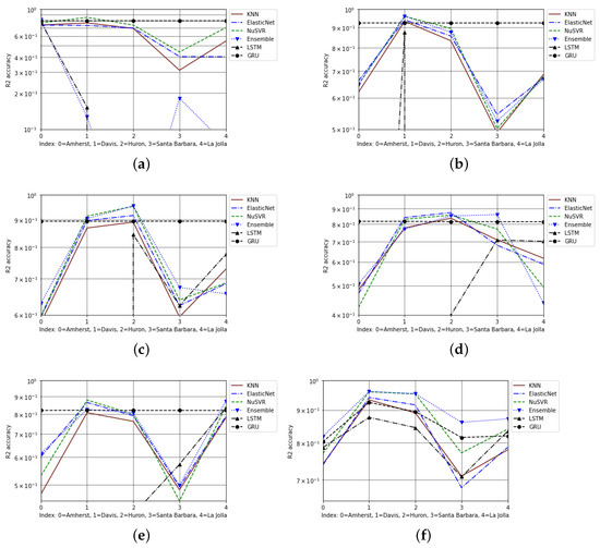
Figure 4.
The cross-city and same-city scores from projections on 3 years, on a semilog scale: (a) Amherst cross-city projections, (b) Davis cross-city projections, (c) Huron cross-city projections, (d) Santa Barbara cross-city projections, (e) La Jolla cross-city projections, (f) same-city projections.
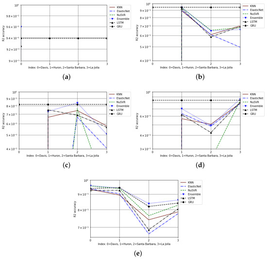
Figure 5.
The cross-city and same-city scores from projection on 6 years, on a semilog scale: (a) Davis cross-city projections, (b) Huron cross-city projections, (c) Santa Barbara cross-city projections, (d) La Jolla cross-city projections, (e) same-city projections.
The results from all the models were compiled, and for easier comprehension, they were selectively tabulated. Only the top 5 performing models of each testing condition were included in Table 1. In this study, the final value used in determining a model’s cross-city performance was obtained by taking the average of all the results of projections including the same-city. Meanwhile, the same-city performance of a model was determined by obtaining the mean of the results from the training and testing phase occurring at the same location. For further readability, Table 2 was constructed based on Table 1. If a model was within the top 5 performances of any given testing condition for same-city or cross-city projections, then a score between one and five, inversely proportional to the ranking of the model, was assigned. If a model had the best performance, it received a score of five, while the fifth best model received a score of one. The models were then reordered based on the decreasing overall performances. When a model did not receive a ranking under any of the test conditions, it was reflected by a dashed line. The process of tabulating the results was repeated for scores across 6 years, and RMSE for 3 and 6 years, as shown in Table 3, Table 4, Table 5, Table 6, Table 7 and Table 8, respectively.

Table 1.
The overall top-performing models, given scores on 3 years of data.
Table 2.
The overall ranking of the top-performing models, given scores on 3 years of data.
Table 3.
The overall top-performing models, given scores on 6 years of data.
Table 4.
The overall ranking of the top-performing models, given scores on 3 years of data.
Table 5.
The overall top-performing models, given RMSE results on 3 years of data.
Table 6.
The overall ranking of the top-performing models, given RMSE results on 3 years of data.
Table 7.
The overall top-performing models, given RMSE results on 6 years of data.
Table 8.
The overall ranking of the top-performing models, given RMSE results on 6 years of data.
For the evaluation metric of scores, the models with the best performances remained relatively similar across datasets spanning 3 and 6 years. Given scores in Table 2 and Table 4, ensemble bagging generalized the best for same-city projections yet also had respectable cross-city forecasts. Meanwhile, GRU had the best projections for cross city for both lengths of datasets. Based on the method for determining the cross-city performance of a model, GRU would be the only model that maintained accuracy across 6 years.
Although the accuracy metrics of MSE and RMSE were obtained, only RMSE is discussed in the report (Figure 6). This is because RMSE is more commonly compared between studies and is derived from MSE. The LSTM was the most accurate model for cross-city projections for RMSE on 3 years of data, as shown in Table 6. Ensemble bagging performed the best given same-city projections, and GRU generalized the best for both conditions between the two models. The better performances of the neural networks could be attributed to the memory storage of previous states inherent in these models. Meanwhile, the performance of the ensemble method could be attributed to the model’s nature averaging the results across the baseline models relying on bootstrapping. Additionally, for RMSE results across 6 years, ensemble bagging had the best generalizations for both same-city and cross-city projections.
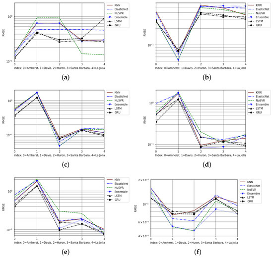
Figure 6.
The cross-city and same-city RMSE results from projections on 3 years, on a semilog scale: (a) Amherst cross-city projections, (b) Davis cross-city projections, (c) Huron cross-city projections, (d) Santa Barbara cross-city projections, (e) La Jolla cross-city projections, (f) same-city projections.
The runtimes of the models were recorded. These runtimes incorporate the training and testing time for each model across 3 and 6 years of length, as displayed in Table 9. The increase in runtimes of the machine learning models from 3 to 6 years is significantly greater than that of the deep learning models compared in the study. The runtimes of the LSTM and GRU increased by a negligible factor, while the machine learning models increased on average by a factor of three. The preprocessing time for both the machine learning and deep learning models increased comparably.
Table 9.
The average runtimes of each of the models when tested on 3 and 6 years.
In this study, the kernel ridge model should be disregarded because the algorithm was not stable. It was common for the model to have cross-city MSE and RMSE results that were magnitudes worse when it was trained on any city and tested on Amherst or Davis. This is most likely caused by overtuning the model as a 10th-degree polynomial kernel was used.
From the extensive testing that was conducted, it became clear that select cities proved to be best for the training or testing phases. For each city, the projections were more accurate when trained and tested on the same city. This contrasts with cross-city projections, where, in each test case, the error is greater than that of the same-city projection. The average of all cross-city projections was derived to evaluate the cumulative cross-city performance for each training city. When conducting cross-city projections, the optimal city used in the training phase was Davis. This is because when a model was trained on a dataset from a city that was not Davis, and tested on Davis, there were disproportionately large inaccuracies in those projections relative to the cross-city projections trained on other cities. This can be visualized in the cross-city projections of Figure 7b–d. Davis is the optimal location to use as a training city because the cumulative accuracy of the cross-city projections was improved when trained on the city. This resulted from mitigating the disproportionately larger inaccuracies when forecasted upon that city. However, if the dataset from the city of Davis was to be omitted, then the best dataset for the training phase for cross-city and same-city projections would be from Huron. Should this research be extended and applied to any given city, such that a model is trained on one city and tested on another, the dataset from the city of Huron should be used during the training phase.
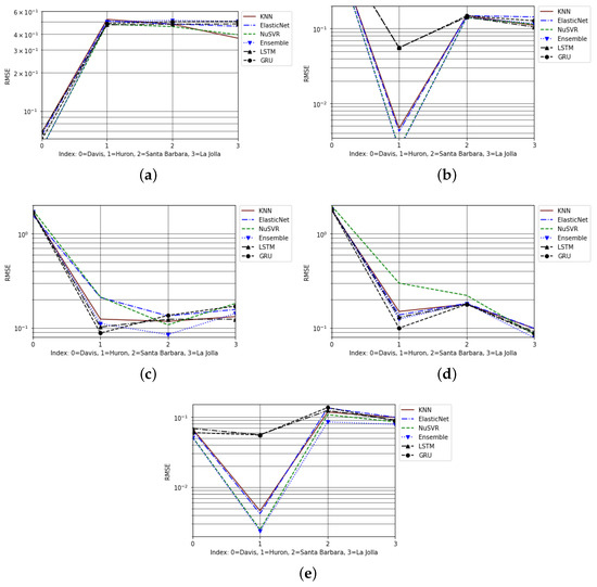
Figure 7.
The cross-city and same-city RMSE results from projections on 6 years, on a semilog scale: (a) Davis cross-city projections, (b) Huron cross-city projections, (c) Santa Barbara cross-city projections, (d) La Jolla cross-city projections, (e) same-city projections.
4. Discussion
Over the past few decades, the installation of PV arrays has increased exponentially. Although benefiting the environment by reducing the consumption of fossil fuels, this surge has primarily been driven by the reduction in costs of these RES. Given the ever-increasing implementation of PVs into electrical systems, and the intricate dependencies these sources have with shading and correlated weather conditions, it is critical that PVs are accurately modeled. Typically, select machine learning and deep learning algorithms have been adapted to model these RES with varied performances. The objective of this study was to compare the accuracy of stochastic models, in particular, neural networks that were implemented against machine learning algorithms to accurately model the output power of PV arrays. This testing was conducted on a dataset that spanned 3 and 6 years in length and was inclusive of five locations. Although the accuracy performances varied based on the testing conditions, the training times for the LSTM and GRU remained relatively constant from 3 to 6 years, in contrast to the other models tested. It was determined that the LSTM and GRU had the best overall performances, and of the two, the GRU outplaced the LSTM when considering scores as well. However, if seeking an algorithm for a single location, ensemble bagging should be selected. That said, the GRU was the most robust of the models when determining the output power of PV arrays in very short-term deterministic forecasts.
Future Works
This application of cross-city projections could be expanded upon and used to model the PV arrays from any given city. This would be particularly beneficial to locations where limited data are available, yet a more extensive dataset available at a different location could be utilized for training. Additionally, this study could be expanded upon by implementing a physical array of sensors to validate the findings, thereby creating a hybridized model. Arrays composed of sensors capable of measuring the highly predictive parameters could be installed in the five given cities and measured simultaneously for the same length of time to accomplish the validation. Should this application be further developed, the dataset from the city of Huron yielded the most accurate projections for modeling alternative cities and, therefore, could be used as a baseline. Additionally, these models and the cross-location projections could be applied to the modeling of other RES, such as onshore or offshore wind farms.
Author Contributions
Conceptualization, M.M.; project administration and advising, Z.Z.; all other sections and contributions, E.S. All authors have read and agreed to the published version of the manuscript.
Funding
Although this research received no external funding, Dr. Ziming Zhang was partially supported by NSF CCF-2006738.
Data Availability Statement
The code, data, and results are available from the forked repository “Modeling-PV-Power-On-6yrs-Spatiotemporal-Data” at https://github.com/Zhang-VISLab?tab=repositories. The data were compiled from sources that permitted their usage as long as they were not for commercial use.
Acknowledgments
We are grateful to Gregory Noetscher, Rodica Neamtu, and Yiqing Zhang from Worcester Polytechnic Institute for their insight and guidance.
Conflicts of Interest
The authors declare no conflict of interest; additionally, the partial funding that Z.Z. received had no influence on this study.
Abbreviations
The following abbreviations are used in this manuscript:
| WPI | Worcester Polytechnic Institute |
| PV | photovoltaic |
| ANN | artificial neural network |
| RES | renewable energy sources |
| NREL | National Renewable Energy Laboratory |
| SIG Energy | Special Interest Groups Energy |
| DHI | diffused horizontal irradiance |
| GHI | global horizontal irradiance |
| LSGDR | linear stochastic gradient descent regressor |
| PLS | partial least squares |
| KNN | k-nearest neighbors |
| SVR | support vector regressor |
| SVM | support vector machine |
| MLP | multilayer perceptron |
| RNN | recurrent neural network |
| LSTM | long short-term memory |
| GRU | gated recurrent unit |
| MSE | mean squared error |
| RMSE | root mean squared error |
References
- Alanazi, M.; Alanazi, A.; Khodaei, A. Long-term solar generation forecasting. In Proceedings of the 2016 IEEE/PES Transmission and Distribution Conference and Exposition (T&D), Dallas, TX, USA, 3–5 May 2016; pp. 1–5. [Google Scholar]
- Agency, I.R. Renewables 2021. Available online: https://www.iea.org/reports/renewables-2021 (accessed on 15 December 2022).
- Masters, G.M. Renewable and Efficient Electric Power Systems; Wiley: New York, NY, USA, 2013. [Google Scholar]
- Ramasamy, V.; Feldman, D.; Desai, J.; Margolis, R. U.S. Solar Photovoltaic System and Energy Storage Cost Benchmarks: Q1 2021; Technical Report; National Renewable Energy Laboratory (NREL): Golden, CO, USA, 2021. [Google Scholar]
- Dolara, A.; Leva, S.; Manzolini, G. Comparison of Different Physical Models for PV Power Output Prediction. Sol. Energy 2015, 119, 83–99. [Google Scholar] [CrossRef]
- Louzazni, M.; Mosalam, H.; Khouya, A.; Amechnoue, K. A Non-Linear Auto-Regressive Exogenous Method to Forecast the Photovoltaic Power Output. Sustain. Energy Technol. Assess. 2020, 38, 100670. [Google Scholar] [CrossRef]
- Ogliari, E.; Dolara, A.; Manzolini, G.; Leva, S. Physical and Hybrid Methods Comparison for the day Ahead PV Output Power Forecast. Renew. Energy 2017, 113, 11–21. [Google Scholar] [CrossRef]
- Nguyen, D.D.; Lehman, B.; Kamarthi, S. Solar Photovoltaic Array’s Shadow Evaluation Using Neural Network with On-Site Measurement. IEEE Trans. Energy Convers. 2007, 10, 44–49. [Google Scholar]
- Wellby, S.J.; Engerer, N.A. Categorizing the Meteorological Origins of Critical Ramp Events in Collective Photovoltaic Array Output. J. Appl. Meteorol. Climatol. 2016, 55, 1323–1344. [Google Scholar] [CrossRef]
- Engerer, N.A. Simulating Photovoltaic Array Performance Using Radiation Observations from the Oklahoma Mesonet. Master’s Thesis, University of Oklahoma, Norman, OK, USA, 2011. [Google Scholar]
- Jewel, U. Limits on cloud-induced fluctuation in photovoltaic generation. IEEE Trans. Energy Convers. 1990, 5, 8–14. [Google Scholar] [CrossRef] [PubMed]
- Rashid, M.H. Power Electronics Handbook, 2nd ed.; Elsevier: Cambridge, MA, USA, 2007. [Google Scholar]
- Mughal, M.A. Machine Learning. 2022. Available online: https://lucid.app/lucidchart/81100e02-09b8-493d-8e66-289665d672f5/edit?invitationId=inv_c62c0815-6391-4479-9516-5481af4c2ec8&page=0_0# (accessed on 12 April 2023).
- Tina, G.M.; Ventura, C.; Ferlito, S.; De Vito, S. A State-of-Art-Review on Machine-Learning Based Methods for PV. Appl. Sci. 2021, 11, 7550. [Google Scholar] [CrossRef]
- Theocharides, S.; Theristis, M.; Makrides, G.; Kynigos, M.; Spanias, C.; Georghiou, G. Comparative Analysis of Machine Learning Models for Day-Ahead Photovoltaic Power Production Forecasting. Energies 2021, 14, 1081. [Google Scholar] [CrossRef]
- Zhu, T.; Guo, Y.; Li, Z.; Wang, C. Solar Radiation Prediction Based on Convolution Neural Network and Long Short-Term Memory. Energies 2021, 14, 8498. [Google Scholar] [CrossRef]
- Glassley, W.; Kleissl, J.; Dam, C.; Shiu, H.; Huang, J. California Renewable Energy Forecasting, Resource Data and Mapping Executive Summary. Public Interest Energy Res. Program 2010, 1–135. [Google Scholar]
- Yona, A.; Senjyu, T.; Saber, A.; Funabashi, T.; Sekine, H.; Kim, C. Application of neural network to 24-hour-ahead generating power forecasting for PV system. In Proceedings of the 2008 IEEE Power and Energy Society General Meeting—Conversion and Delivery of Electrical Energy in the 21st Century, Pittsburgh, PA, USA, 20–24 July 2008; pp. 1–6. [Google Scholar]
- Ding, S.; Li, R.; Tao, Z. A novel adaptive discrete grey model with time-varying parameters for long-term photovoltaic power generation forecasting. Energy Convers. Manag. 2021, 227, 113644. [Google Scholar] [CrossRef]
- Severiano, C.A.; Candido de Lima e Silva, P.; Cohen, M.W.; Guimaraes, F.G. Evolving fuzzy time series for spatiotemporal forecasting in renewable energy systems. Renew. Energy 2021, 171, 764–783. [Google Scholar]
- Liu, C.; Gu, J.; Yang, M. A Simplified LSTM Neural Networks for One Day-Ahead Solar Power Forecasting. IEEE Access 2021, 9, 17175–17178. [Google Scholar] [CrossRef]
- Markovics, D.; Mayer, M. Comparison of machine learning methods for photovoltaic power forecasting based on numerical weather prediction. Renew. Sustain. Energy Rev. 2022, 151, 112364. [Google Scholar] [CrossRef]
- Sengupta, M.; Xie, Y.; Lopez, A.; Habte, A.; Maclaurin, G.; Shelby, J. The National Solar Radiation Data Base (NSRDB). Renew. Sustain. Energy Rev. 2018, 89, 51–60. [Google Scholar] [CrossRef]
- Energy, S.I.G. Energy Systems and Informatics. 2023. Available online: https://energy.acm.org/resources/ (accessed on 20 March 2023).
- NREL. NSRDB: National Solar Radiation Database. 2023. Available online: https://nsrdb.nrel.gov/data-viewer/ (accessed on 20 March 2023).
- Science, U.A.C. Cumulative Inverter Performance. 2023. Available online: http://s38210.mini.alsoenergy.com/Dashboard//2a566973506447764241554b772b71593d (accessed on 20 March 2023).
- DGStats, C. CSI 15-Min Interval Data. 2023. Available online: https://www.californiadgstats.ca.gov/downloads/ (accessed on 20 March 2023).
- Singh, S. Solar Irradiance Concepts: DNI, DHI, GHI & GTI. 2022. Available online: https://www.yellowhaze.in/solar-irradiance/ (accessed on 15 December 2022).
- Oceanic, N.; Administration, A. Dew Point vs. Humidity. 2023. Available online: https://www.weather.gov/arx/why_dewpoint_vs_humidity (accessed on 27 March 2023).
- DBpedia. Solar Zenith Angle. 2022. Available online: https://dbpedia.org/page/Solar_zenith_angle (accessed on 15 December 2022).
- Service, C.G.L. Surface Albedo. 2020. Available online: https://land.copernicus.eu/global/products/sa (accessed on 15 December 2022).
- Abubakar Mas’ud, A. Comparison of three machine learning models for the prediction of hourly PV output power in Saudi Arabia. Ain Shams Eng. J. 2022, 13, 2–5. [Google Scholar] [CrossRef]
- Yale. Linear Regression. 1998. Available online: http://www.stat.yale.edu/Courses/1997-98/101/linreg.htm (accessed on 27 March 2023).
- Shi, A. SGDRegressor with Scikit-Learn: Untaught Lessons You Need to Know. 2023. Available online: https://towardsdatascience.com/sgdregressor-with-scikit-learn-untaught-lessons-you-need-to-know-cf2430439689#:~:text=The%20SGDRegressor%20algorithm%20uses%20stochastic,with%20respect%20to%20the%20parameters (accessed on 27 March 2023).
- Lumivero. Partial Least Squares. 2023. Available online: https://www.xlstat.com/en/solutions/features/partial-least-squares-regression#:~:text=The%20Partial%20Least%20Squares%20regression,used%20to%20perfom%20a%20regression.&text=Some%20programs%20differentiate%20PLS%201,is%20only%20one%20dependent%20variable (accessed on 27 March 2023).
- University, P.S. Ridge Regression. 2018. Available online: https://online.stat.psu.edu/stat857/node/155/ (accessed on 27 March 2023).
- Learn Developers, S. Scikit Learn Kernel Ridge. 2023. Available online: https://scikit-learn.org/stable/modules/generated/sklearn.kernel_ridge.KernelRidge.html#:~:text=Kernel%20ridge%20regression%20(KRR)%20combines,function%20in%20the%20original%20space (accessed on 27 March 2023).
- Godwin, J.A. Ridge, LASSO, and Elastic Net Regression. 2021. Available online: https://towardsdatascience.com/ridge-lasso-and-elasticnet-regression-b1f9c00ea3a3 (accessed on 27 March 2023).
- MathWorks. Lasso and Elastic Net. 2022. Available online: https://www.mathworks.com/help/stats/lasso-and-elastic-net.html (accessed on 2 April 2023).
- Mukherjee, D.; Chakraborty, S.; Kumar Gucchait, P.; Bhunia, J. Machine Learning Based Solar Power Generation Forecasting with and without an MPPT Controller; IEEE Xplore: Piscataway, NJ, USA, 2020; pp. 44–46. [Google Scholar]
- Raj, A. A Quick and Dirty Guide to Random Forest. 2020. Available online: https://towardsdatascience.com/a-quick-and-dirty-guide-to-random-forest-regression-52ca0af157f8 (accessed on 6 April 2023).
- Sampling with Replacement and Sampling without Replacement. 2023. Available online: https://web.ma.utexas.edu/users/parker/sampling/repl.htm (accessed on 6 April 2023).
- Bishop, C.M. SVMs for Regression. In Pattern Recognition and Machine Learning; Springer: New York, NY, USA, 2006; pp. 338–345. [Google Scholar]
- Learn Developers, S. NuSVR. 2023. Available online: https://scikit-learn.org/stable/modules/generated/sklearn.svm.NuSVR.html (accessed on 27 March 2023).
- Learn Developers, S. Neural Network Models (Supervised). 2023. Available online: https://scikit-learn.org/stable/modules/neural_networks_supervised.html (accessed on 27 March 2023).
- Keras. Adadelta. 2012. Available online: https://keras.io/api/optimizers/adadelta/ (accessed on 27 March 2023).
- Kostadinov, S. Understanding GRU Networks. 2017. Available online: https://towardsdatascience.com/understanding-gru-networks-2ef37df6c9be (accessed on 27 March 2023).
- Gupta, A. Grated Recurrent Unit Networks. 2023. Available online: https://www.geeksforgeeks.org/gated-recurrent-unit-networks/ (accessed on 27 March 2023).
- Willmott, C.J.; Ackleson, S.G.; Davis, R.E.; Feddema, J.J.; Klink, K.M.; Legates, D.R.; O’Donnell, J.; Rowe, C.M. Statistics for the evaluation and comparison of models. Energies 1985, 90, 8995–9005. [Google Scholar] [CrossRef]
- Frost, J. Multicollinearity in Regression Analysis: Problems, Detection, and Solutions. 2020. Available online: https://statisticsbyjim.com/regression/multicollinearity-in-regression-analysis/ (accessed on 6 April 2023).
- Desmos. Why Am I Seeing a Negative R2 Value? 2020. Available online: https://help.desmos.com/hc/en-us/articles/202529139-Why-am-I-seeing-a-negative-R-2-value-#:~:text=In%20practice%2C%20R2%20will,the%20mean%20of%20the%20data (accessed on 6 April 2023).


Disclaimer/Publisher’s Note: The statements, opinions and data contained in all publications are solely those of the individual author(s) and contributor(s) and not of MDPI and/or the editor(s). MDPI and/or the editor(s) disclaim responsibility for any injury to people or property resulting from any ideas, methods, instructions or products referred to in the content. |
© 2023 by the authors. Licensee MDPI, Basel, Switzerland. This article is an open access article distributed under the terms and conditions of the Creative Commons Attribution (CC BY) license (https://creativecommons.org/licenses/by/4.0/).