Abstract
Photovoltaic generation is one of the key technologies in the production of electricity from renewable sources. However, the intermittent nature of solar radiation poses a challenge to effectively integrate this renewable resource into the electrical power system. The price reduction of battery storage systems in the coming years presents an opportunity for their practical combination with utility-scale photovoltaic plants. The integration of properly sized photovoltaic and battery energy storage systems (PV-BESS) for the delivery of constant power not only guarantees high energy availability, but also enables a possible increase in the number of PV installations and the PV penetration. A massive data analysis with long-term simulations is carried out and indicators of energy unavailability of the combined system are identified to assess the reliability of power production. The proposed indicators allow to determine the appropriate sizing of the battery energy storage system for a utility-scale photovoltaic plant in a planning stage, as well as suggest the recommended operating points made for each month through a set of graphs and indicators. The presence of an inflection zone has been observed, beyond which any increase in storage does not generate significant reductions in the unavailability of energy. This critical zone is considered the sweet spot for the size of the storage, beyond which it is not sensible to increase its size. Identifying the critical point is crucial to determining the optimal storage size. The system is capable of providing reliable supply of constant power in monthly periods while ensuring capacity credit levels above 95%, which increases the penetration of this renewable resource. Despite the fact that the study focuses exclusively on the analysis from an energy perspective, it is important to consider the constraints associated to real storage systems and limit their oversizing.
1. Introduction
Energy systems are undergoing a transition process towards a new paradigm, characterized by electrification of the economy, decarbonization (gradual reduction of carbon intensity) of energy generation parks, and decentralization of energy resources. The electrical system has to guarantee the electrical supply, i.e., energy, but also the quality of this supply, which must be carried out at the lowest possible cost. In addition, environmental protection is becoming increasingly important.
By 2050, electricity could become the central energy carrier, growing from a 20% share of the final consumption to an almost 50% share; as a result, gross electricity consumption would more than double [1]. The analysis [2] has already indicated that it is possible to eliminate almost all CO2 emissions by 2050 and partially replace fossil fuels in transport and heating. The capacity for electricity generation from renewable sources, in particular photovoltaic solar energy, is growing remarkably [3].
In an initial phase of this transition, emphasis has been placed on obtaining energy (MWh). Renewable energy system technologies have focused mostly on taking advantage of the maximum power of renewable energy resources. These systems are already mature and competitive, and it is already widely recognized that their generation cost is lower compared to the traditional generation systems. However, large-scale renewables pose a challenge for grid operations [4,5]. As they are dependent on natural resources and, therefore, variable and intermittent, they cannot ensure their availability to start operating when energy is needed, but only when there are enough resources, meaning they are not dispatchable. As long as the penetration of renewables is low, this is manageable and can be accepted by the electricity system operators. In 2021, 22% of the energy consumed in the European Union was generated from renewable sources, according to EEA early estimates. The long-term prospects may still fall short of the current 32% renewable energy target set for 2030 [6]. However, as the share of renewable energy generation grows, the power systems face challenges related to both system flexibility and system stability (ability of power systems to withstand disturbances on a very short time scale) [3]. In this context, smart grids are defined as an electric power system that integrates the behavior and actions of the network users and other stakeholders, to efficiently deliver sustainable, economic, and secure electricity supplies. The grid utilizes information exchange and control technologies, distributed computing, and associated sensors and actuators for those purposes but also all the network users (consumers, generators, storage owners) must be able to act in a network-friendly manner. Therefore, it is increasingly important that renewable energy generation helps maintain system reliability and stability, and this may be increasingly required by interconnection standards. The concept of hosting capacity is used to study how much photovoltaic power can be placed on a feeder before the negative effects appear on the normal operation of the distribution system and power quality (overvoltages/undervoltages and voltage variations) [5]. Hosting capacity is typically expressed as the megawatt value of distributed photovoltaic (PV) at any location on the feeder, which causes the first violation of operating restrictions. The voltage level definition in different regions varies. In Europe, the EN-50160 standard establishes the limits of ±10% of the nominal voltage. In the Americas, the ANSI C84.1 standard is followed, which imposes more restrictive limits of ±5% of nominal voltage.
On the other hand, a plant’s contribution to the security of supply is not measured by its installed power, but rather by the power it can offer at times of peak demand with minimal security or certainty. This “safe” power is called firm power. Firmness is understood as the maximum power that can be overcome by a certain high level of probability. The firm power depends on factors such as the availability of primary energy used (fuel, wind, water, etc.) and the maintenance carried out on the installation or its operating regime (number of stops/starts, etc). So far, the firmness is a characteristic of manageable technologies such as nuclear power or gas, which do not depend on external agents, and are attributed with firmness coefficients greater than 95% [7]. This, however, is not true for renewable technologies without storage, especially wind and photovoltaic power, since they fully depend on the availability of resources, meaning that the electricity generation that they will be able to contribute to the system at a specific moment in time cannot be predicted with certainty in the medium term. The firmness cycle of wind energy is usually considered to be 9%, whereas the value for photovoltaic solar energy (without storage) lies at 0% [8]. The classic approach to addressing the variability problem of renewable energy installations is to add flexible resources, such as large generators and Volt–Amps Reactive (VAR) control equipment. Thermal technology, especially gas turbine combined cycles (CCGTs), is currently the best at providing a backup service with a lower level of greenhouse gas emissions. Specifically, the greatest advantage offered by this technology is its ability to quickly start, regulate, or stop its operation in order to accommodate the input of clean energy.
Another aspect to consider is that in a scenario of high penetration of renewable technologies in the system, especially when using solar energy, simultaneous generation of renewable energy can trigger overgeneration at noon and create a risk that a part of electricity will not be incorporated into the system due to low demand, thus going to waste, which is known as curtailments.
Through the combination of PV plants with storage systems, photovoltaic installations can be endowed with firmness, enabling greater integration into electrical networks. Power generation in hybrid PV systems with storage is more predictable, controllable, and dispatchable, or, in other words, more grid friendly [9]. The integration of battery energy storage systems (BESS) in photovoltaic plants brings reliability to the renewable resource and increases the availability to maintain a constant power supply for a certain period of time. Ref. [10] shows a forecast in which a combination of storage and solar power can reach 30 TWh worldwide by 2050, far exceeding any other storage capacity.
From the point of view of hosting capacity, the power to be taken into account for the PV-BESS would no longer be the peak power of the collection field, but rather the constant power that it guarantees to deliver to the network. This could also increase the number of installations that fit into a certain distribution network, sometimes restricted in the interconnection agreements established by the electricity distribution companies. In this process, the most unfavorable effect is usually considered, in which the power generated by the photovoltaic plant is the maximum possible power that can be injected, usually the maximum power of the inverter, despite the fact that photovoltaic systems only work at full power 5% of the time. In this way, the capacity of the network is underused in practice. On the other hand, through the combination between PV and BESS, it is possible to achieve that; for example, ten 1 MWp plants can be integrated into the electric grid instead of just one 1 MWp plant, thus producing constant power of 100 kW.
In addition to providing firmness, storage can reduce curtailment and valorize photovoltaic energy, avoiding the feared cannibal effect that can hinder economic viability of photovoltaic installations when their penetration is high [11].
The use of batteries has a significant impact on strengthening photovoltaic generation and improving primary frequency control. It is important to note that there is a restriction on the instantaneous power supply capacity provided by the storage system and its corresponding inverters. In the present study, no emphasis was placed on the analysis of the primary frequency control, since its operation is in time ranges of seconds. The simulations carried out have been designed with the purpose of analyzing energy balances in hourly intervals.
The optimal sizing of a photovoltaic plant with a storage system is a subject widely studied in scientific literature. Refs. [12,13,14,15] investigate the optimal sizing of PV and BESS systems in an electric grid. Many studies of PV and BESS focus part of their work on analyzing economic viability. The main parameters to analyze are the annual production of photovoltaic energy, the useful life of the components and the costs of the installation (Capital Expeditures (CapEx), Operational expeditures (OpEx), and Operation and Maintenance (O&M)) [16,17,18,19]. Cost projections for utility-scale lithium-ion battery systems estimate reductions of 28–58% by 2030 and 28–75% by 2050 [20]. At present, the large-scale manufacturing of batteries for their use in electric vehicles is contributing to the reduction of prices [21]. However, this paper does not consider economic factors, but rather focuses on determining the optimal operation of a photovoltaic–battery energy storage system (PV-BESS) from the point of view of energy analysis, based on sizing parameters of the system. The objective of the PV-BESS proposed is to achieve capacity credit similar to those plants that provide firm power to the electrical network. Therefore, in the sizing and operation of the system, indicators will be assigned in search of reaching a capacity credit of around 95%.
In ref. [22], it is concluded that before policy makers make decisions about the nature of future electricity grids, it is necessary to re-examine the role of technologies to provide baseload capacity. It is imperative to consider a diversity of renewable supply options. One of the possible approaches could promote the use of intermittent or variable energy sources as alternatives to current baseload generation technologies, through the use of electricity storage systems [23]. The case proposed in this study presents similarities with concentrated technology solar power (CSP), and in ref. [23] it is stated that, in terms of costs, baseload-capable CSP could become competitive with nuclear power by 2030 if it sees sufficient deployment to drive costs down. There are numerous techno-economic studies that seek to minimize the installation cost or avoid the economic penalties associated with deviations in the intraday market, through forecast methodologies based on deep learning. Refs. [24,25] are some representative examples.
However, the purpose of this study is to present a novel vision in which the minimization of storage costs is not emphasized, but rather seeks to ensure long-term firm capacity, since a drastic reduction in storage costs is expected in a future scenario.
In a previous paper [26], the size of the most suitable storage system for a given panel power in Wp has been shown, together with the selection of the firm power with which it is desired to operate, on an annual basis, which can be delivered with a firmness of 95%, i.e., a less than 5% probability that the firm power cannot be delivered every hour of the year. However, with the annual setpoint, there is a high amount of excess energy that is not incorporated into the network in the months of high irradiation (surplus), thus reducing the economic viability of the plant as these kWh are not sold, and, on the other hand, the amount of clean kWh that can be incorporated into the network is reduced. For this reason, this paper presents a different operating strategy, called Monthly Constant Power. The objective of sizing based on storage size and power supplied in this particular case is focused on guaranteeing, with a probability greater than 95%, a specific power setpoint value that has been optimized for each month of the year. Massive data analysis over a long simulation period has made it possible to identify the degree of robustness of the system and determine an optimal storage size. By identifying that there is no linear relationship between the increase in storage capacity and the reduction in unavailability of energy, it is necessary to analyze the results obtained to find the optimal configuration.
The article is structured as follows: Section 2 exposes the methodology used to provide a firm capacity in monthly periods, including its characteristic parameters and indicators, which are necessary to carry out the analysis. Section 3 describes the proposed model that is used to determine various suitable sizings for the PV-BESS system. Section 4 presents the results obtained from simulations, discussing the most relevant conclusions provided by the unavailability curves and Load Duration Curves. Finally, a summary with the main conclusions is presented in Section 5.
2. Methods
2.1. System Parameters and Indicators
The storage capacity of the PV-BESS system is defined based on the parameter storage to power ratio (S2P), which is calculated using Equation (1). In this equation, CBESS represents the storage capacity of the system (MWh) and PPV is the peak power of the photovoltaic installation (MWp). The S2P parameter is equivalent and is used as a measure of autonomy hours in isolated photovoltaic installations.
The capacity factor of a plant is the ratio between the theoretical maximum energy production of the plant and its actual energy production over a certain period of time [27]. For a one-year period, it is the quotient between the photovoltaic production of the plant EPV,AN (MWh) and peak power of the plant PPV (MW) for the 8760 h in a year, as shown in Equation (2).
As an example, Equation (2) shows the calculation of the capacity factor (CF), taking into account the photovoltaic production data resulting from the statistical calculations developed in Section 2.2.
The typical capacity factor in plants with intermittent renewable energy such as wind or solar power is strongly site-dependent and is usually between 15% and 40% [28].
In Equation (3), the equivalent operating factor of the system (CPOF) is calculated, where PGRID represents the constant power to be supplied to the network and PPV represents the peak power of the photovoltaic installation.
To guarantee the supply of a firm power, it is necessary that the operation factor provided by the system is less than that associated with the average annual production proposed in Equation (2). If the aforementioned is not met, the photovoltaic installation would present a deficit net annual energy that would be impossible to cover by the PV-BESS.
In case in a certain hourly interval the system cannot supply the required energy to the electrical network EGRID, there will be an energy deficit in the PV-BESS, since neither the storage system nor the photovoltaic plant will be able to provide the necessary energy.
The unavailability of energy in the system is quantified by means of the energy deficit (ED) indicator.
In Equation (4), the energy deviation (ED) is defined as a relative accumulator of unavailable energy throughout the entire simulation period, where the numerator represents the unavailable energy and the denominator represents the energy supplied during the entire simulation period. EPV represents the photovoltaic production for each hour, EGRID represents the energy supplied each hour and h represents the number of hourly periods of the simulation.
If the ED indicator is equal to zero, the system ideally meets the demanded power setpoint and there is no energy unavailability. To obtain the average annual unavailability, the Annual Energy Deficit (AED) indicator will be used, which will take the average data of all simulation years. If it is desired to disaggregate energy unavailability according to the month of the year, the Monthly Energy Deficit (MED) indicator will be used, which will take only the data for the month in question.
The aforementioned parameters and indicators maintain a commonly used criterion with respect to [26], in which a constant power study was carried out under annual instructions.
2.2. Proposed Methodology
The generation of energy by a photovoltaic installation is presented as a function of time, since it depends on the amount of solar radiation received on the surface of the solar panels. However, the estimates present a certain margin of uncertainty, since it also depends on the atmospheric conditions and the efficiency of the system. In order to homogenize the hourly production in a large-scale PV, the adequate sizing of a storage system and the identification of optimal operating points for each month are proposed, in order to guarantee a firm-power supply. Indicators of power unavailability quantify the reliability of the system in the long-term simulation. In this context, the physical limitations of the system and the energy losses are considered and a model is established that allows to identify, for each hour, the distribution of energy in the system.
Figure 1 shows a comparison between the power supplied by a photovoltaic plant (blue dashed line) and the power setpoint that is intended to be supplied during a full day in January (in red) in p.u. The per-unit value of any quantity is defined as the ratio of actual value in any unit to the base or reference value in the same unit. The horizontal axis represents the time in hours for a random day of the simulation, while the vertical axis represents the power in per unit with respect to the peak power of the photovoltaic installation (1 MWp). The energy supplied by the photovoltaic plant shows fluctuations throughout the day due to variations in solar radiation and other factors. The red line is the energy setpoint that is intended to be supplied to the electrical network, constant throughout the day.
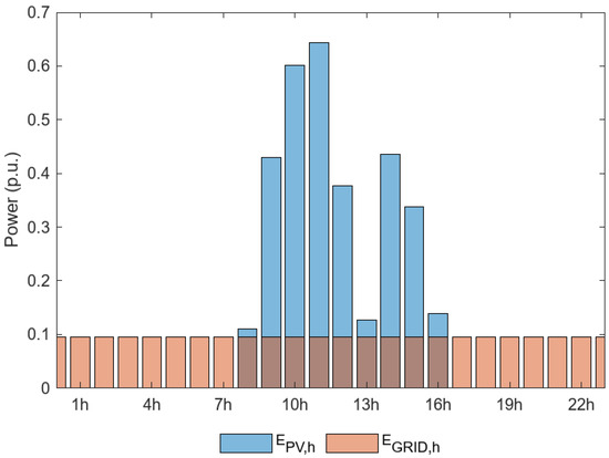
Figure 1.
Comparison between PV installation energy and energy to be supplied to the electrical system.
It can be seen that at certain times of the day, the power supplied by the photovoltaic plant (PPV,H) is less than the setpoint power (PGRID,H) that is intended to be supplied, indicating that the power generation system needs the support of a storage system to maintain a constant output power. At other times, the supplied power is greater than the power setpoint, which indicates that the system is generating more energy than necessary and can store it in the BESS for later use.
The objective of the script programmed in Matlab is to maximize the energy supplied to the electrical network through the PV-BESS system that meets a constant power setpoint. This objective is sought to be achieved under balanced sizing criteria.
Ideally, it would seek to convert all intermittent renewable energy into a system capable of providing constant firm power to the electrical grid. In Figure 1, this would be achieved by matching the area under the curve that represents the photovoltaic production with the power that is intended to be supplied to the grid. In this way, it would ensure that the power supplied is constant and does not depend on fluctuations in the generation of renewable energy. In practice, however, this can be difficult to achieve due to the variability of the renewable resource and the oversizing that would have to be done to the storage system.
A collection of long-term PV production data is a useful tool to identify behavior patterns in a PV plant. These patterns tend to cancel out the fluctuations that occur over short hourly horizons. By using a script in Matlab, the photovoltaic production is grouped by months for a period of 11 years of simulation. This grouping process involves separating the photovoltaic production data into groups corresponding to each of the 12 months of the year. The grouping of monthly data allows the identification of seasonal patterns in the production of photovoltaic energy, useful to propose an adequate dimensioning of the PV-BESS system.
Figure 2 shows the average hourly production (over 11 years) of a photovoltaic plant located in Zaragoza (Spain) for each month of the year. This figure is useful for identifying long-term patterns and trends. Seasonal fluctuations are significant in energy production and are due to the angle of inclination of the Sun’s rays on the Earth. During the summer season, the tilt of the Earth’s axis causes the region in which the photovoltaic plant is located to receive a greater amount of direct solar radiation, resulting in higher energy production. In contrast, during the winter season, the region in which the photovoltaic plant is located receives less direct solar radiation, which results in lower energy production.
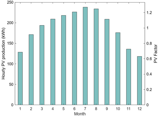
Figure 2.
Hourly photovoltaic production and PVFACTOR coefficient for each month of the year.
The seasonal variation in photovoltaic production is identified by means of a dimensionless index or coefficient for each month of the year. This coefficient will be used to model the expected production of photovoltaic energy for any month of the year. Although in short hourly periods, the uncertainty of PV production is high, in the long term, the dimensionless coefficient is precise and reliable since it has been obtained from a very long-term statistical analysis.
PVFACTOR is called the dimensionless coefficient obtained from the statistical analysis of the solar energy production of a photovoltaic plant and it is represented on the ordinate axis on the right in Figure 2. This coefficient is expressed in per unit, being the sum of the values for all the months of the year equal to 12. PVFACTOR results from dividing the average monthly production for a certain month with respect to the annual production. A greater PVFACTOR indicates that the solar energy production in that month is greater compared to other months of the year and vice versa.
As it has been said, the purpose is to match a renewable source facility, which has an intermittent resource, with power plants that supply firm power to the system, such as nuclear power plants, which have a reliable resource. Therefore, the energy supplied per hour is required to be constant, in order to ensure the continuity of the electrical supply and minimize possible interruptions or unavailability thereof.
The appropriate selection of the hourly energy setpoint is one of the fundamental keys to achieving an adequate dimensioning of the installation. In this sense, the implemented algorithm applies an hourly power setpoint to be supplied to the electrical network (PGRID) proportional to the photovoltaic production of each month according to the PVFACTOR mentioned in Figure 2.
The power reference supplied by the system (PGRID) is calculated through Equation (5), where PPV represents the peak power of the photovoltaic installation and CPOF is the operating factor of the plant.
As an example, Figure 3 shows the constant monthly power that the system must supply when selecting a CPOF setpoint value equal to 0.1 or 0.14 with a 1 MWp photovoltaic plant. These represented values will be useful for later comparison with results from Section 4.1.
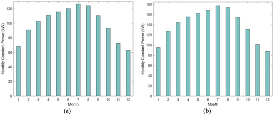
Figure 3.
Constant monthly power setpoint (a) CPOF = 0.1; (b) CPOF = 0.14.
3. Model of the PV-BESS
A script was developed using the Matlab numerical computing software, developed by MathWorks, to model the behavior of a photovoltaic plant with battery energy storage. Matlab was selected due to its efficiency in processing large, structured databases using vector operations.
The created script performs hourly energy balance computations over a period of 11 years (96,360 time slots), which requires hundreds of millions of operations due to the more than 1200 combinations of battery size and power setpoint that must be considered. To reduce the execution time of the script, the matrix-organized vector operation was used, which allowed the data to be processed more efficiently. As a result, the script can carry out the necessary calculations in a reasonable amount of time, making it easy to get accurate and reliable results.
The PV-BESS facility is located in Zaragoza, Spain, at a latitude of 41.65°. The monocrystalline photovoltaic panels are fixed on the roof with an optimized inclination of 35° towards the south. The simulated photovoltaic installation has a capacity of 1 MWp. The battery energy storage system (BESS) uses lithium-ion batteries with a depth of discharge (DoD) of 90%. In the simulations, the nominal capacity of the storage system varies up to 6 MWh with increments of 0.1 MWh. The battery discharge curve is C1, considering a self-discharge coefficient of 5%. The efficiency of the equivalent photovoltaic inverter is 90%, while the efficiency of the inverter associated with storage is 91% [29,30]. Lithium iron phosphate batteries are used, scalable up to 6 MWh and 6 MW with a cycle life of 10,000 cycles for a depth of discharge of 80% [31]. The manufacturer declares a calendar life greater than 10 years. When evaluating using the rainflow-counting method, 4369 equivalent cycles are recorded depending on the state of charge (SoC) and the depth of discharge (DoD) throughout the simulation, as shown in Figure 4. Since the end of life of the storage is still far away, the degradation does not decisively affect the simulation results.
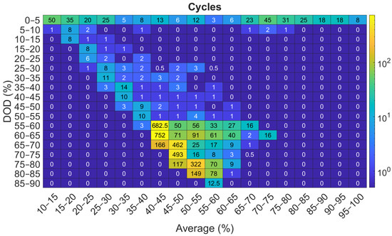
Figure 4.
Number of equivalent cycles depending on SoC and DoD.
To describe the degradation resulting from charge and discharge cycles, the term cycling aging is used. The main factors contributing to an increase in degradation are indicated as follows. High temperatures cause an accelerated degradation of the storage system. Given that current BESSs are equipped with cooling systems, this factor has been overlooked, assuming an average temperature within the BESS of 25 °C. Each charge or discharge cycle is associated with an average state of charge and a depth of discharge, as shown in Figure 4. The sum of the cycles corresponding to each depth of discharge and average SoC yields the overall degradation of the storage system. High values of state of charge result in a loss of active lithium, although its influence is reduced compared to the degradation by depth of discharge. In relation to the proposed case, the battery manufacturer’s datasheet [31] provides the degradation for each cycle number segment of Figure 4.
The battery manufacturer’s datasheet indicates that it is possible to achieve battery depths of discharge of up to 90%. However, it is important to note that it should not be common as it involves subjecting the storage to high degradation stress. The analysis carried out using the rainflow-counting algorithm method allows to identify the number of cycles that occur in each level of discharge. As can be seen in Figure 4, it is unusual for charge and discharge cycles to be performed around a DoD of 90%. Therefore, storage degradation would not experience critical deterioration due to this circumstance. The manufacturer guarantees more than 7000 cycles for a DoD of 0.9 as stated in [31].
The energy balance of the installation is performed by discretizing values into hourly intervals over a period of 11 years. The simulation has been designed to include enough time slots to allow considering the operation of the representative system at the proposed location. The representation of the system is shown in Figure 5, where a diagram is shown that allows a clear visualization of the configuration of the system.
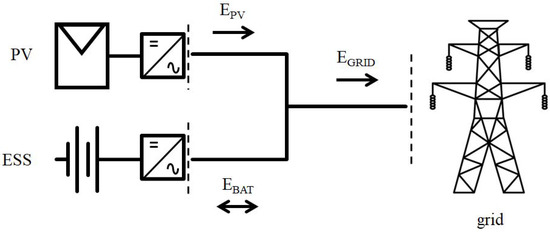
Figure 5.
Diagram of the PV-BESS system.
For the simulation, climatological values were extracted in hourly time slots between January 2006 and December 2016 by using the Photovoltaic Geographical Information System web tool [32]. This tool has made it possible to obtain reliable information on the climate at the location of the installation. The climatological values obtained make it possible to calculate the photovoltaic production and include hourly information on the average solar radiation on the photovoltaic plane (GM) and ambient temperature (TA). The temperature of the photovoltaic cell (TC) is calculated using Equation (6), where NOCT is the nominal operating cell temperature of the photovoltaic cell [33,34], and it was considered to be 47 °C.
The power produced by a photovoltaic module (PMOD) is calculated according to Equation (7). This equation considers the nominal power of the photovoltaic module (PN), the irradiance under standard measurement conditions (GSTC), and the temperature coefficient of the photovoltaic panel (γ), which was considered to have a value of 0.35%·K−1 [33,34].
The power produced by the photovoltaic installation (PPV) is obtained according to Equation (8), where NP is the number of photovoltaic panels and CLOSS the coefficient of losses associated with the photovoltaic plant estimated in a photovoltaic plant according to the Photovoltaic Geographical Information System (PVGIS) [32].
The proposed script operates in hourly time slots with energy units (Wh). The energy balance for each time slot can be formalized by Equation (9), where EPV is the energy produced by the photovoltaic installation for a given hour and TS is a time slot corresponding to 1 h.
If the power supply EPV is insufficient to maintain the setpoint of energy delivered to the electrical grid (EGRID) in a given time slot, the storage system must supply the remaining power. To calculate the energy extracted from the storage system (EBAT,dis), Equation (10) is used, where EBAT, dis is the energy drawn or discharge from the storage system in the current time slot, EGRID is the energy demanded by the electrical network in the current time slot, ηIN is the efficiency of the inverters associated with the photovoltaic modules, ηBAT is the efficiency of the inverters associated with the storage system, σ is the self-discharge coefficient of the storage system [35], and EBAT,h-1 is the energy stored in the storage system in the previous time slot. In summary, this equation calculates the amount of energy that must be extracted from the storage system to meet the energy demand of the electrical network in the current time slot [36].
If the power supply from the photovoltaic panels (EPV) is higher than the energy setpoint to be delivered to the electrical grid (EGRID), energy is stored in the storage system. The amount of energy that is stored (EBAT, cha) is calculated by Equation (11), where EBAT, cha is the energy introduced into the storage system in the current time slot [36].
The Matlab script that has been proposed is responsible for organizing the data extracted from PVGIS and the equations presented in a matrix. Each row of the matrix represents a time slot of one hour and, sequentially, the energy balance is calculated for each time slot. The variables shown in Table 1 are represented in each column of the matrix.

Table 1.
Summary of input variables to the algorithm matrix.
The script operation in Matlab to perform the net energy balance in the storage system (EBAT) is carried out at each hour of the day, according to Equation (12). This equation uses as input the energy stored in the system in the previous hour (EBAT,h−1). However, to apply Equation (12), it is necessary to comply with certain restrictions related to the operating ranges of the batteries and inverters of the photovoltaic and battery energy storage system (PV-BESS). These restrictions are detailed in Table 2 and are considered by the algorithm in each energy balance calculation. In this way, safe and optimal operation of the storage system is guaranteed and overload situations are prevented.
Table 2.
Physical restrictions associated with the PV-BESS system.
After applying the operating restrictions of the storage system, the net balance of hourly energy (EBAT) is calculated and added to the matrix as another column. In the simulation, the BESS state of charge (SOC) is initialized to a value of 55% of the nominal value of the storage system. This initialization is done to ensure that the SOC is within the safe operating range of the storage system and there are no constraints in the early hours of the simulation that could affect the AED or MED indicators.
The dimensioning of the system is modified by varying the CPOF and S2P parameters, which makes it possible to obtain representative indicators of the unavailable energy in search of the optimal AED or MED. The simulation is carried out over a period of 11 years, which guarantees a significant average of the behavior of the system over time. Figure 6 shows the flowchart of the algorithm programmed in Matlab used to perform the simulation.
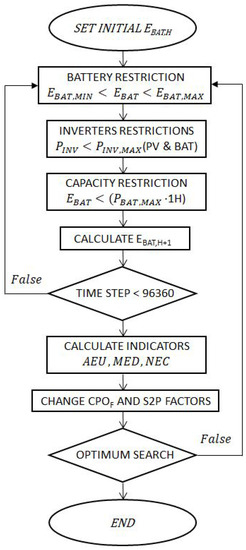
Figure 6.
Flowchart of the algorithm programmed in Matlab.
4. Results
As discussed in Section 2, the purpose of this case study is to analyze the proper sizing of an installation with photovoltaic panels and battery storage. The system must supply the electrical network with a constant power set point every hour (EGRID). The power supplied to the electrical grid is optimized and varied monthly to adapt to fluctuations in photovoltaic production, as proposed in Section 2. In order to reach a solid set of conclusions, a sizing analysis is carried out, which is based on two independent approaches. The first one is based on the use of the AED or MED indicators in relation to the S2P and CPOF parameters. The second approach consists of the analysis of the generation duration curves of the system. These complementary approaches make it possible to obtain a broad vision of the proper dimensioning of the system.
The generation duration curves represent the distribution of power generation over time, showing the hours in which a constant power is maintained by the PV-BESS. By identifying the flat area or the number of hours that firm power is maintained, it is possible to confirm the suitability of the system.
The results obtained from the AED or MED indicators, as well as from the analysis of the generation duration curves, make it possible to identify the appropriate values of the S2P and CPOF parameters. By considering a wide range of values for these parameters, it is possible to evaluate different scenarios and select those that provide optimal and satisfactory sizing. To achieve this goal, a Matlab simulation was carried out using irradiance data at hourly intervals over a period of 11 years. The purpose of analyzing this extensive series of simulated data is to obtain a volume of results representative of the operation of the system. The irradiance data were obtained from the PVGIS database [32].
4.1. Analysis of the AED Indicator
The evaluation of non-compliance with the constant power supply of the PV-BESS installation is carried out by quantifying the unavailable energy in hourly intervals throughout the entire simulation period. Consequently, the Annual Energy Deviation (AED) indicator presented in Section 2 is used to measure the energy deficit of the facility.
Figure 7 shows the AED values for different CPOF power setpoints according to its storage size (S2P). The purpose of this figure is to provide a visual representation of how the AED indicator values vary with different power setpoints and storage sizes. This information is essential to identify the optimal combination of power setpoints and storage sizes that provide energy performance with guarantees of reduced energy unavailability.
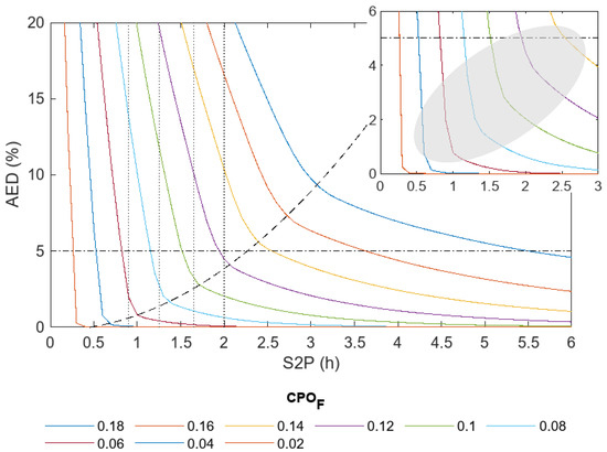
Figure 7.
AED for monthly constant power.
Initially, all the curves represented in Figure 7 show a rapid decrease of the AED indicator as the storage size (S2P) increases. However, in all the curves there is an inflection point from which increases in storage size do not produce significant reductions in the AED indicator. Joining this critical point for each curve in Figure 7 forms a black dashed line whose trajectory resembles an exponential function. This critical point is considered the sweet spot for the size of the storage, beyond which it does not make sense to increase its size. Identifying the critical point is critical to determining the optimal storage size.
To ensure a high firmness of the PV-BESS system, it is proposed to keep the AED indicator below 5%, which is equivalent to establishing a capacity credit of 95% as proposed in Section 1. Consequently, the adequate dimensioning of the system to each curve in Figure 7 is defined as the one in which the AED indicator is less than 5% and is in the vicinity of the mentioned saturation knee point. To accurately identify the most favorable operating points of the system, the area of greatest interest is zoomed in on in Figure 7. A gray shaded area has been delimited that indicates the most beneficial possible operating points of the system. The points identified in the shaded area have the two conditions mentioned in common. First, they are below an AED index value of 5%, as shown by the dot-dash line. Secondly, these points are located in the vicinity of the saturation curve that is observed in the dashed line.
For Figure 7 and considering the curve corresponding to a CPOF of 0.12, it can be seen that to reduce the AED indicator from 7.5% to 5%, it is necessary to increase the S2P index from 1.77 h to 1.94 h, which represents an increase in storage size of 9.6%. However, if you want to reduce the AED indicator by the same percentage level (from 3.5% to 1%), you need to increase the S2P index from 2.24 h to 4.11 h, which implies an increase in storage size of 83.4%. Therefore, it is crucial to select a system operation in zones that are to the left of the saturation knee identified in Figure 7, in order to avoid unnecessary oversizing of storage. According to the mentioned criteria, some examples of suitable sizing can be identified in Figure 7, above the dashed dotted line. In particular, the 1 MWp photovoltaic plant guarantees that a capacity credit greater than 95% (equivalent to an AED index of less than 5%) is supplied, by selecting the following constant power storage and setpoint combinations: CPOF = 0.12 and S2P = 2 h; CPOF = 0.1 and S2P = 1.65 h; CPOF = 0.08 and S2P = 1.25 h; CPOF = 0.06 and S2P = 0.9 h.
As defined in Section 2, note that a CPOF value of 0.12 is associated with the supply of an average annual constant power of 120 kW. On the other hand, an S2P value of 2.2 h implies the use of storage with a capacity of 2.2 MWh.
To verify the optimization of the system through the monthly adjustment in the power setpoint, a comparison is made between two systems in Figure 8. The first system supplies constant power throughout the year, as already discussed in [26]. The second system adjusts the power setpoint monthly to adapt to the photovoltaic production. In the Figure 8 legend, next to each CPOF value, it is indicated whether the setpoint is an annual setpoint (A) or varies depending on the month (M). Although the monthly setpoint varies, at the end of the year it represents the same CPOF than the constant setpoint, since the setpoint increases in months of high photovoltaic production and are offset by a reduction in months of lower photovoltaic production. Therefore, the CPOF in the monthly setpoint (M) is equivalent to the annual setpoint (A) and they can be compared.
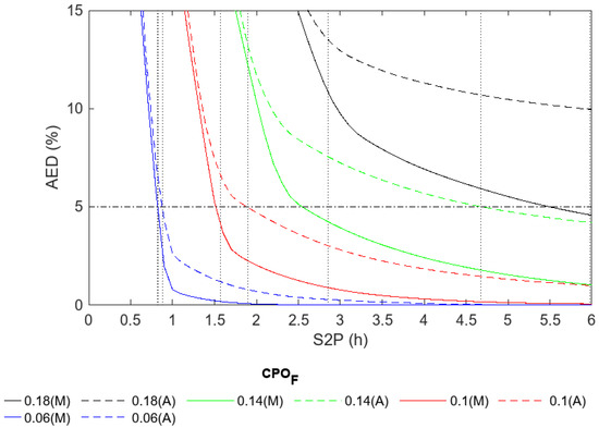
Figure 8.
Comparison of AED indicator for monthly and annual constant power setpoint.
For reduced values of constant power (CPOF of 0.06), it can be seen in the blue curves of Figure 8 that there is a minimal variation in the AED indicator, and the monthly setpoint barely improves AED. For example, to ensure AED of 5%, the annual constant power requires an S2P of 0.87 h, while the monthly constant power requires slightly less storage with an S2P of 0.82 h.
For high values of constant power, a significant improvement is observed when using a monthly setpoint instead of an annual setpoint. For example, for a CPOF of 0.10, the annual target requires an S2P of 1.9 h to maintain an AED of 5%, while the monthly target only requires an S2P of 1.57 h as seen in Figure 8. For a CPOF of 0.14, the use of a monthly constant power instead of a yearly constant power significantly reduces the S2P from 4.68 h to 2.85 h, which is equivalent to nearly halving the required storage. The use of a CPOF very high and close to the total photovoltaic production generated would be unfeasible with an annual constant power operation, as shown in the black curve in Figure 8. However, with a monthly setpoint operation, it would be viable with high storage (S2P = 5.9 h).
4.2. MED Indicator Analysis
Section 2 formulated the MED indicator to disaggregate the energy deficits of the system by months, according to Equation (4). Figure 9 illustrates the MED indicator for the most significant months of the year. The photovoltaic production in December presents a minimum value, while in July it reaches its maximum value. April and October have intermediate values.
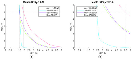
Figure 9.
Comparison of the MED indicator: (a) Case with CPOF of 0.1; (b) Case with CPOF of 0.14.
Figure 9a shows the MED indicator for an intermediate power reference (CPOF = 0.1). It is worth clarifying that a CPOF of 0.1 implies that the average firm power setpoint for all months of the year is 10% of the installation’s peak power. In the box corresponding to the figure, the constant power that is being supplied each specific month is specified. However, to each of the MED curves in Figure 9, the PVFACTOR coefficient and Equation (5) are also applied. Therefore, for the case of CPOF of 0.1 in December the minimum firm power of 62.79 kW is reached and in July, it reaches 126.61 kW due to the monthly correction factor PVFACTOR shown in Figure 2 and Figure 3a.
It Is observed that, in the month of December, the MED indicator is clearly more unfavorable for any storage size. The identification of the month with the least capacity to satisfy the energy demand is crucial to establish the most restrictive conditions for the design and operation of the system. Meeting a maximum MED indicator of 5% requires an S2P storage of 1.9 h in the month of December, while for the rest of the year, an S2P storage of 1.5 h would suffice. The average of the MED indicator for the 12 months of the year is equivalent to the AED in Figure 7, whose value is 1.57 h. Therefore, for a CPOF of 0.1, it is proposed to size the BESS with an S2P of 1.57 h that meets a capacity credit of 95% every month except December. However, if you want to select the most restrictive conditions imposed by the month of December, S2P must be 1.9 h.
For a high power setpoint (CPOF = 0.14), the MED indicator presents more accentuated differences, as can be seen in Figure 9b. December remains the most critical month in terms of renewable energy storage requirements and July remains the most favorable. The box corresponding to Figure 9b corresponds to the monthly constant power setpoints that are represented in Figure 3b.
To keep the MED rate below 5% with a CPOF power setpoint of 0.14 in July, S2P renewable energy storage of 2.39 h would be required, as shown in Figure 9b. This indicates that, during the month of July, the energy demand can be met with a smaller size of energy storage compared to other months of the year. However, in December, more energy storage (S2P of 5.45 h) would be required to keep the MED ratio below 5%. These results highlight the importance of considering seasonal variations in photovoltaic production. The selection of an S2P of 2.85 h to keep the AED below 5% in Figure 7 implies that an annual average of less than 5% would be met on an annual average. However, as previously indicated in Figure 9b, in the month of December, an S2P value of 5.45 h would be necessary to keep the MED ratio below 5%. This means that, in some months of the year, especially those in which photovoltaic production is minimal, an S2P value significantly higher than that indicated by the AED may be necessary to guarantee capacity credit above 95%. Therefore, it is important to consider both the annual value of the AED and the monthly variability of the MED index when selecting the value of S2P if capacity credits greater than 95% are sought each month [26].
The situation described suggests expanding the study with the optimization of the PVFACTOR index from Equation (5), in order to achieve a balance in the MED index and ensure similar energy deficits each month. The objective would be to increase the power setpoint in months of high photovoltaic production (June to August) and reduce the power setpoint in months of low photovoltaic production (November to January). In this study, a direct correlation has been established between the photovoltaic production of the plant and the constant power that must be supplied for each month. However, for future research, the use of genetic algorithms is proposed to analyze an optimal PVFACTOR for each month, through massive hourly data processing.
It can be seen In Figure 9a that the monthly constant power value can be optimized for dimensioning with CPOF = 0.1 and S2P = 3 h. In the month of July, the MED index is zero. This indicates that the batteries have a wide operating margin and the power setpoint could be increased in July, ensuring a MED of less than 5%.
By increasing the power setpoint in July, the power setpoint in December can be reduced in the same proportion, which would reduce both the global unavailability throughout the year and the unavailability in December.
4.3. Generation Duration Curves Comparison
It is common to use Generation Duration Curves (GDC) to represent the generation capacity of power plants. In the GDCs, the magnitude to be represented is arranged in descending order instead of doing it chronologically. The maximum load is plotted to the left of the curve, and successive loads are plotted in descending order as you move to the right of the curve.
The area under the GDC represents the energy supplied by the system and, in the cases proposed in this section, allows analyzing the availability of energy or the capacity of use of the system. The vertical axis of the GDC represents the hourly energy available to be supplied to the electrical network (EGRID), while the horizontal axis represents the percentage of time of the entire simulation in which that energy can be supplied.
The goal is to provide a different perspective to the AED or MED indicator, which measure the amount of unavailable power in the system. Instead, it is proposed to analyze the time during which there is energy availability in the system as an alternative indicator.
When selecting a monthly power reference with a CPOF of 0.1, several simulations were carried out varying the storage capacity (S2P) in order to analyze the power that the PV-BESS system delivers to the electrical network (EGRID). Figure 10 shows the results of these simulations. In the GDC, an almost flat zone is observed corresponding to the time in which a constant power is being supplied to the electrical system.
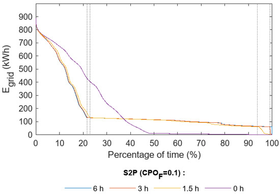
Figure 10.
Generation duration curves with CPOF of 0.1, varying S2P.
The curve corresponding to S2P = 0 h in Figure 10 represents a system without storage, and it is the only one that does not present a flat zone in the GDC. In this case, the delivery of constant power to the electrical system cannot be guaranteed, and the energy supplied to the electrical grid corresponds directly to the generated photovoltaic energy. Decreasing power supply is guaranteed up to almost half of the simulation period.
In Figure 10, the curve for S2P = 1.5 h shows that the system is capable of supplying constant power up to 93.8% of the simulation period. From S2P = 3 h, it is guaranteed that more than 99% of the simulation period the target power is supplied. However, it is important to note that increasing S2P does not necessarily imply a reduction of excess energy with respect to the constant power reference. In the curves corresponding to SP2 of 1.5 h, 3 h, and 6 h of Figure 10, a minimal variation in the excess energy of the system is observed. During up to 22.8% of the simulation period, excess energy occurs with respect to the power set point.
It may be convenient to reduce the photovoltaic production by adjusting the operating point of the photovoltaic inverter in the event that an excess of energy supplied to the grid may imply penalties. In this way, constant power could be guaranteed in the period in which the energy surplus is obtained, which in this case corresponds to the time frame up to 22.8% of the simulation period, as observed in the curves for S2P of 1.5 h, 3 h, and 6 h of Figure 10.
Proper selection of storage size (S2P) is essential to optimize the number of hours in which constant power can be guaranteed throughout the simulation period. The GDCs shown in Figure 11 illustrate the number of hours that the system is capable of supplying the energy demanded by the electrical grid (EGRID) for different storage levels, including low, medium, and high.
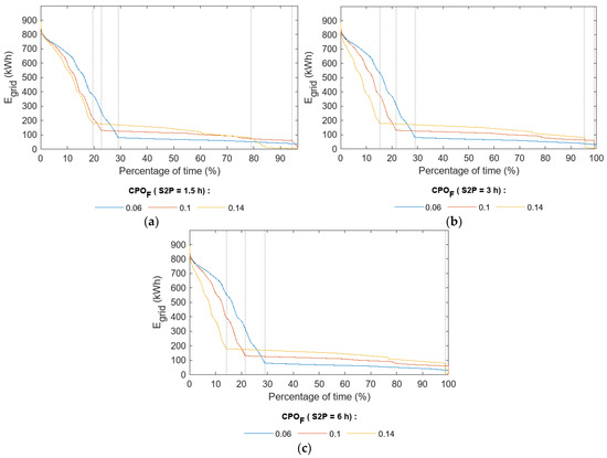
Figure 11.
Generation duration curves with various CPOF: (a) Case S2P of 1.5 h (low capacity of the BESS); (b) Case of S2P of 3 h, medium capacity or the BESS; (c) Case of S2P of 6 h, high capacity of the BESS.
Figure 11a aims to represent the influence of the CPOF parameter for a low storage value (S2P = 1.5 h). For a CPOF of 0.06, the constant power value is guaranteed during the entire simulation period (>99% of the time). Increasing the CPOF at 0.1, you could keep the power value constant up to 94.3% of the time. For a constant high power with a CPOF of 0.14, the supply is guaranteed for 78.9% of the time.
In Figure 11b, the storage value is increased to an intermediate level (S2P = 3 h). With a CPOF of 0.06 and 0.1, the constant power can be supplied most of the time. For a CPOF of 0.14, constant power can be maintained for 95.1% of the time. Therefore, increasing the value of S2P compared to Figure 11a generally increases the number of hours that constant power can be supplied for each CPOF.
Figure 11c represents an oversizing of the storage system with a value of S2P equal to 6. For the values of CPOF as shown, it can be seen that constant power can be guaranteed practically throughout the simulation time, due to the significant reduction in energy deficits that involves using the backup of a very large storage system.
As has been noted, the increase in S2P increases the number of hours in which the monthly constant power can be maintained, which seems logical since the storage system acts as a backup. However, it is significant that in the three graphs of Figure 11, it is observed that increasing storage (S2P) hardly reduces excess energy. Excesses of energy are distinguished because EGRID does not present a flat shape in the GDC. For a CPOF of 0.06, the three storage sizes maintain a constant level of excess energy of 29.1%. for a CPOF of 0.1, the excess energy is around 21%. Only for the CPOF of 0.14, there is a variation in the excess energy between 14.2% and 19.5%.
In Figure 7, it has been shown that, for a CPOF of 0.1, selecting a storage capacity that is twice the installed peak power of the photovoltaic plant (S2P = 2 h) guarantees a capacity credit of 95%. In Figure 11, it is confirmed that for a CPOF of 0.1, with an S2P storage size of 3 h or 6 h, constant power (>99%) can be delivered virtually all the time. Only for S2P = 1.5 h, availability is reduced to 94.3% of the time. In conclusion, the values of S2P from 1.5 h to 3 h are an adequate sizing to guarantee a high-capacity credit while maintaining a CPOF of 0.1.
Using the battery manufacturer’s datasheet [31], the degradation is identified in each segment of the rainflow-counting method, resulting in an average of 1.7% degradation. This quantitative indicator provides a general estimate of the loss of efficiency and capacity of the storage system due to the degradation factors identified throughout the charge and discharge cycles. Such small degradation percentages do not have a significant influence on the ED indicators of the system.
5. Conclusions
This paper proposes an adequate sizing and operation of a system formed by a photovoltaic plant and a battery storage system in order to provide firmness to photovoltaic power generation. The system model has been described, indicating its corresponding parameters and indicators.
A long-term simulation was carried out using Matlab software in order to identify the indicators of unavailability. The simulation was carried out through massive vector data computation, which enabled the analysis of large amounts of operations in a short period of time.
The power setpoint was adjusted for each month of the year, based on the expected photovoltaic production. The objective was to guarantee a constant power supply or a capacity credit of 95%.
According to the simulation results, the photovoltaic plant guarantees a supply of an annual capacity credit of more than 95%, and does so by selecting combinations of constant power setpoint and storage ranges around the following values: CPOF = 0.12 and S2P = 2 h, CPOF = 0.1 and S2P = 1.65 h, or CPOF = 0.06 and S2P = 0.9 h.
If the month with the lowest photovoltaic production is considered, S2P must be oversized with respect to an annual analysis that meets a 95% capacity credit. For example, for a CPOF of 0.1, it is proposed to size the BESS with an S2P of 1.57 h (AED < 5%). However, the analysis of the more restrictive conditions imposed by the month of December (MED < 5%) shows that S2P should be oversized to 1.9 h. The analysis of the Load Duration Curves confirmed that for an intermediate power set point with CPOF of 0.1 and a large storage size with S2P between 3 h and 6 h, constant power can be supplied practically all the time (>99%). Reducing the storage size to S2P = 1.5 h reduces the system availability to 94.3% of the time. It can be concluded that S2P values between 1.5 h and 3 h are adequate sizing. With adequate monthly power setpoints, the AED and MED indicators are improved. The case study is specific to a specific geographic location; however, all the conditions and equations of the model have been identified so that they can be reproduced in any scenario and hourly period by introducing an irradiance and temperature matrix in hourly periods. Batteries are experiencing a drastic drop in costs, and this trend is expected to continue. Therefore, in this study, an attempt was made to make an abstraction of the conventional techno-economic analyses that are commonly found in the bibliography. The objective was not the minimization of storage costs, but the identification of a suitable point of operation that avoids unnecessary oversizing of the storage system. The energy analysis carried out reveals the existence of a saturation zone or elbow from which, for each power set point, it is not justified to increase the storage capacity, since no significant improvements are observed in the reduction of energy unavailability. Although the study was carried out for a particular case, its results can be extrapolated to any scenario that involves the combination of photovoltaic systems and energy storage systems. This is due to the fact that the algorithm used was designed in a general way, and it would only be necessary to make modifications in the specific parameters of the system to adapt it to each particular case.
Within the framework of ongoing research and considering future lines of work, we established the objective of incorporating a detailed analysis of degradation phenomena. This approach will provide a clear view of the charge and discharge processes, as well as their degradation.
Author Contributions
Conceptualization, J.A.T.-G. and Á.A.B.-R.; methodology, J.A.T.-G. and Á.A.B.-R.; software, J.A.T.-G.; validation, J.A.T.-G. and Á.A.B.-R.; formal analysis, J.A.T.-G.; investigation, J.A.T.-G. and Á.A.B.-R.; resources, J.A.T.-G.; data curation, J.A.T.-G.; writing—original draft preparation, J.A.T.-G. and Á.A.B.-R.; writing—review and editing, Á.A.B.-R.; visualization, J.A.T.-G.; supervision, Á.A.B.-R.; project administration, Á.A.B.-R.; funding acquisition, Á.A.B.-R. All authors have read and agreed to the published version of the manuscript.
Funding
This research received no external funding.
Data Availability Statement
Not applicable.
Conflicts of Interest
The authors declare no conflict of interest. The funders had no role in the design of the study; in the collection, analyses, or interpretation of data; in the writing of the manuscript, or in the decision to publish the results.
Abbreviations
| PV-BESS | Photovoltaic plants with Battery Energy Storage Systems |
| PV | Photovoltaic |
| EEA | European Environment Agency |
| VAR control | Volt–Amps Reactive control |
| CCGTs | Combined-Cycle Gas Turbines |
| BESS | Battery Energy Storage System |
| CapEx | Capital Expenditures |
| OpEx | Operational Expenditures |
| O&M | Operation and Maintenance |
| CSP | Concentrated Solar Power |
| S2P | Storage to Power ratio (h) |
| CBESS | Capacity of Battery Energy Storage System (MWh) |
| PPV | Peak Power of Photovoltaic plant (MW) |
| CF | Capacity Factor (%) |
| EPV,AN | Annual Energy production (MWh) |
| CPOF | Constant Power Operation Factor (p.u.) |
| PGRID | Power to be supplied to the grid (MW) |
| EGRID | Energy to be supplied to the grid (MWh) |
| ED | Energy Deficit indicator (p.u.) |
| EPV | Energy production of Photovoltaic plant |
| AED | Annual Energy Deficit indicator |
| MED | Monthly Energy Deficit indicator |
| PVFACTOR | Monthly photovoltaic factor (p.u.) |
| DoD | Depth of Discharge of BESS (%) |
| SoC | State of Charge of BESS (%) |
| GM | Average solar radiation on the photovoltaic plane (W · m−2) |
| TA | Ambient temperature (°C) |
| TC | Temperature of the photovoltaic cell (°C) |
| NOCT | Nominal Operating Cell Temperature (°C) |
| PMOD | Power produced by a photovoltaic module (W) |
| PN | Nominal power of the photovoltaic module (W) |
| GSTC | Irradiance under standard test conditions (W · m−2) |
| γ | Temperature coefficient of photovoltaic module (% · K−1) |
| NP | Number of photovoltaic modules |
| CLOSS | Coefficient of losses associated with photovoltaic plant (p.u.) |
| TS | Time slot (h) |
| EBAT,dis | Energy discharging BESS (MWh) |
| ηIN | Efficiency photovoltaic inverter (%) |
| ηBAT | Efficiency BESS inverter (%) |
| σ | Self-discharge coefficient of BESS (p.u.) |
| EBAT,h-1 | Energy in BESS in the previous time slot (MWh) |
| EBAT,cha | Energy charging of BESS (MWh) |
| EBAT,MAX | Maximum capacity of the BESS (MWh) |
| EBAT,MIN | Minimum capacity of the BESS (MWh) |
| PINV(PV),MAX | Maximum power of the photovoltaic inverters (MW) |
| PINV(BAT),MAX | Maximum power of the battery inverters (MW) |
| PBAT | BESS Power (MW) |
| GDC | Generation Duration Curve |
References
- IRENA. Global Energy Transformation: A roadmap to 2050 (2019 Edition); International Renewable Energy Agency: Abu dhabi, United Arab Emirates, 2019. [Google Scholar]
- European Commision, COM. 112 Final Communication A Roadmap for Moving to a Competitive Low Carbon Economy in 2050; European Commision: Ispra, Italy, 2011. [Google Scholar]
- IEA. Getting Wind and Sun onto the Grid. A Manual for Policy Makers; ODCE-IEA: Paris, France, 2017. [Google Scholar]
- Bayod-Rújula, A.A. Future development of the electricity systems with distributed generation. Energy 2009, 34, 377–383. [Google Scholar] [CrossRef]
- Palmintier, B.; Robert, B.; Barry, M.; Michael, C.; Kyri, B.; Fei, D.; Matthew, R.; Matthew, L.; Ashwini, B. Emerging Issues and Challenges in Integrating Solar with the Distribution System; NREL: Golden, CO, USA, 2016. [Google Scholar]
- European Environment Agency. Available online: https://www.eea.europa.eu/ims/share-of-energy-consumption-from (accessed on 9 May 2023).
- Statista. Available online: https://www.statista.com/statistics/191201/capacity-factor-of-nuclear-power-plants-in-the-us-since-1975 (accessed on 25 January 2023).
- CNMC. Propuesta de Orden por la que se Establece la Regulación del Pago por Capacidad Establicido en la Ley 54/1997 de 27 de Noviembre; National Energy Comision CNE: Santiago, Chile, 2007. [Google Scholar]
- Bayod-Rújula, A.A.; Haro-Larrode, M.; Martínez-Gracia, A. Sizing criteria of hybrid photovoltaic–wind systems with battery storage and self-consumption considering interaction with the grid. Sol. Energy 2013, 98, 582–591. [Google Scholar] [CrossRef]
- International Energy Agency. World Energy Outlook 2022; IEA: Paris, France, 2022. [Google Scholar]
- López Prol, J.; Steininger, K.W.; Zilberman, D. The cannibalization effect of wind and solar in the California wholesale electricity market. Energy Econ. 2020, 85, 104552. [Google Scholar] [CrossRef]
- Blasuttigh, N.; Negri, S.; Massi Pavan, A.; Tironi, E. Optimal Sizing and Environ-Economic Analysis of PV-BESS Systems for Jointly Acting Renewable Self-Consumers. Energies 2023, 16, 1244. [Google Scholar] [CrossRef]
- Hassan, Q.; Pawela, B.; Hasan, A.; Jaszczur, M. Optimization of Large-Scale Battery Storage Capacity in Conjunction with Photovoltaic Systems for Maximum Self-Sustainability. Energies 2022, 15, 3845. [Google Scholar] [CrossRef]
- Korjani, S.; Casu, F.; Damiano, A.; Pilloni, V.; Serpi, A. An online energy management tool for sizing integrated PV-BESS systems for residential prosumers. Appl. Energy 2022, 313, 118765. [Google Scholar] [CrossRef]
- Liao, J.-T.; Chuang, Y.-S.; Yang, H.-T.; Tsai, M.-S. BESS-Sizing Optimization for Solar PV System Integration in Distribution Grid. IFAC-PapersOnLine 2018, 51, 85–90. [Google Scholar]
- Rivera-Durán, Y.; Berna-Escriche, C.; Córdova-Chávez, Y.; Muñoz-Cobo, J.L. Assessment of a Fully Renewable Generation System with Storage to Cost-Effectively Cover the Electricity Demand of Standalone Grids: The Case of the Canary Archipelago by 2040. Machines 2023, 11, 101. [Google Scholar] [CrossRef]
- Han, X.; Garrison, J.; Hug, G. Techno-economic analysis of PV-battery systems in Switzerland. Renew. Sustain. Energy Rev. 2022, 158, 112028. [Google Scholar] [CrossRef]
- Aziz, A.S.; Tajuddin, M.F.N.; Zidane, T.E.K.; Su, C.-L.; Alrubaie, A.J.; Alwazzan, M. Techno-economic and environmental evaluation of PV/diesel/battery hybrid energy system using improved dispatch strategy. Energy Rep. 2022, 8, 6794–6814. [Google Scholar] [CrossRef]
- Gupta, R.; Soini, M.C.; Patel, M.K.; Parra, D. Levelized cost of solar photovoltaics and wind supported by storage technologies to supply firm electricity. J. Energy Storage 2020, 27, 101027. [Google Scholar] [CrossRef]
- Cole, W.; Frazier, A.W.; Augustine, C. Cost Projections for Utility-Scale Battery Storage: 2021 Update; National Renewable Energy Laboratory: Golden, CO, USA, 2021. [Google Scholar]
- Gordon, D. Battery Market Forecast to 2030: Pricing, Capacity and Supply and Demand; E Source Companies LLC.: Carbon Pl Boulder, CO, USA, 2022. [Google Scholar]
- Matek, B.; Gawell, K. The Benefits of Baseload Renewables: A Misunderstood Energy Technology. Electr. J. 2015, 28, 101–112. [Google Scholar] [CrossRef]
- Pfenninger, S.; Keirstead, J. Comparing concentrating solar and nuclear power as baseload providers using the example of South. Energy 2015, 87, 303–314. [Google Scholar] [CrossRef]
- Beltran, H.; Cardo-Miota, J.; Segarra-Tamarit, J.; Perez, E. Battery size determination for photovoltaic capacity firming using deep learning irradiance forecasts. J. Energy Storage 2021, 33, 102036. [Google Scholar] [CrossRef]
- Thanh, N.T.; Huu, V.X.S.; Hieu, D.D.; Tanako, H.; Tuyen, N.D. Short-term PV power forecast using hybrid deep learning model and Variational Mode Decomposition. In Proceedings of the 3rd International Conference of Power and Electrical Engineering, Singapore, 29–31 December 2022. [Google Scholar]
- Bayod-Rújula, Á.A.; Tejero-Gómez, J.A. Analysis of the Hybridization of PV Plants with a BESS for Annual Constant Power Operation. Energies 2022, 15, 9063. [Google Scholar] [CrossRef]
- Wilson, S.; Lightfoote, S.; Voss, S. Evaluation of Solar Capacity Factor of 2000 Solar Plants Across the United States Using Multilayer Perceptron Regressor Models. In Proceedings of the IEEE 49th Photovoltaics Specialists Conference (PVSC), Philadelphia, PA, USA, 5–10 June 2022; pp. 1347–1349. [Google Scholar]
- Green, A.; Diep, C.; Dunn, R.; Dent, J. High Capacity Factor CSP-PV Hybrid Systems. Energy Procedia 2015, 69, 2049–2059. [Google Scholar] [CrossRef]
- Ketjoy, N.; Chamsa-ard, W.; Mensin, P. Analysis of factors affecting efficiency of inverters: Case study grid-connected PV systems in lower northern region of Thailand. Energy Rep. 2021, 7, 3857–3868. [Google Scholar] [CrossRef]
- Khan, M.R.; Alam, I.; Khan, M.R. Inverter-Less Integration of Roof-Top Solar PV with Grid Connected Industrial Drives. Energies 2023, 16, 2060. [Google Scholar] [CrossRef]
- Datasheet Battery Lithium Iron-Phosphate PowerBrick+ 1280Wh from PowerTech. Available online: https://www.powertechsystems.eu/home/products/24v-lithium-battery-pack-powerbrick/50ah-24v-lithium-ion-battery-pack-1-28kwh-powerbrick-lithium/ (accessed on 9 May 2023).
- Photovoltaic Geographical Information System (PVGIS). EU Science Hub. Available online: https://ec.europa.eu/jrc/en/pvgis (accessed on 29 April 2023).
- Borunda, M.; Ramírez, A.; Garduno, R.; Ruíz, G.; Hernandez, S.; Jaramillo, O.A. Photovoltaic Power Generation Forecasting for Regional Assessment Using Machine Learning. Energies 2022, 15, 8895. [Google Scholar] [CrossRef]
- Obaro, A.Z.; Munda, J.L.; Yusuff, A.A. Modelling and Energy Management of an Off-Grid Distributed Energy System: A Typical Community Scenario in South Africa. Energies 2023, 16, 693. [Google Scholar] [CrossRef]
- Can Duman, A.; Salih Erden, H.; Gülen, O. Optimal sizing of PV-BESS units for home energy management system-equipped households considering day-ahead load scheduling for demand response and self-consumption. Energy Build. 2022, 267, 112164. [Google Scholar] [CrossRef]
- Yang, H.; Gong, Z.; Ma, Y.; Wang, L.; Dong, B. Optimal two-stage dispatch method of household PV-BESS integrated generation system under time-of-use electricity price. Int. J. Electr. Power Energy Syst. 2020, 123, 106244. [Google Scholar] [CrossRef]


Disclaimer/Publisher’s Note: The statements, opinions and data contained in all publications are solely those of the individual author(s) and contributor(s) and not of MDPI and/or the editor(s). MDPI and/or the editor(s) disclaim responsibility for any injury to people or property resulting from any ideas, methods, instructions or products referred to in the content. |
© 2023 by the authors. Licensee MDPI, Basel, Switzerland. This article is an open access article distributed under the terms and conditions of the Creative Commons Attribution (CC BY) license (https://creativecommons.org/licenses/by/4.0/).