Abstract
Our current energy landscape is ever-changing, resulting from the ongoing energy transition and introducing a massive expansion of volatile generation feed-in and energy consumption (due to electrification). In turn, the energy supply’s requirements are also being affected. In this context, the energy system’s optimisation across all sectors will only grow in significance, especially in terms of future developments. Facilitating and researching methods for carrying out the aforementioned optimisation creates new demands pertaining to load flow simulation programmes. The volatility of specific participants and their interactions within existing power grids must be evaluated, wherefore the consideration of a large number of time steps but also dynamic simulations becomes inevitable. Carrying out such simulations is possible but very time-consuming. This article compared a variety of conventional load flow simulations such as the current iteration and Newton–Raphson methods and also introduced a novel, state-space based calculation approach, which boasts the potential of structurally increasing simulation speeds. Each of the method’s underlying principles, requirements, and mathematical correlations will be discussed and explained. In the second part of this article, the most important state-space equivalent circuit models of critical operating equipment are introduced. These models are essential for carrying out load flow simulation tests for an exemplary test network but could also be used for dynamic purposes. The previously showcased load flow methods were applied to a test network, with which the simulation methods should be validated. The results show that the state-space simulation has high accuracy while also being very flexible. All in all, the load flow calculation in state-space offers many advantages that could be an interesting alternative to conventional load flow simulations, especially for the analysis of complex, time series-based, and intelligently controlled smart grid power systems. In this context, the direct application of system theoretical methods for stability calculations, controllability, and dynamic system studies is to be mentioned. Optimisation options regarding the processes within the state-space calculation software still promise further significant increases in performance.
1. Introduction
Energy systems are in a constant state of transformation, moving away from a uniform, centralised, and predictable structure towards a decentralised, highly volatile, complex structure. This complexity transfers to the simulation models, in which the assumption of continuous consumption and generation no longer applies. The variable feed-in resulting from the increasing use of renewable energies, such as wind or PV, as well as the dynamic consumption behaviour resulting from new technologies, such as e-mobility and heat pumps, must be taken into account. The increasing number of harmonics, arising from the increased use of inverters, must also be accounted for [1]. The loading behaviour can be considered by using standardised load profiles or by including measured time series in the simulation models. This enables the modelling and predicting of the network behaviour for different conditions. In modern load flow simulation programs, well-known methods, such as Newton–Raphson, are usually used. These methods allow the calculation of all network conditions by solving a system of equations. However, the algorithms used to solve these systems of equations have a certain weakness, especially regarding simulations with large sets of load profiles. The repetitive process of establishing matrices for each time step takes its toll and increases the required simulation time. Frequency-dependent simulations, such as those needed for the evaluation of inverters, also require other substitute models and calculation methods. In this paper, a calculation method is presented that is intended to meet the requirements of modern load flow problems.
2. Energy Grids
The existing grids have grown historically and have a clear structure in which the energy is generated at the highest voltage levels (high and extra-high voltage) and then distributed to the lower voltage levels (medium and low voltage). A distinction is made between the transmission grid (110 kV to 380 kV) and the distribution grid (230 V to 110 kV). The electrical energy was mainly generated in large power plants, which were primarily built in places with corresponding loads, often heavy industry around mining and the steel industry. This explains why, for example, the majority of German power plants are located in the west (NRW) or in the east (Brandenburg). The ever-increasing interconnection of the systems was intended to increase system reliability in addition to the actual energy transport. The main task of the grids was and is to ensure security of supply, system reliability, and stability. In addition, transmission losses should be minimised. In order to ensure high quality, reliability, and safety in electricity transmission and distribution, the grid operators continuously take measures to keep the frequency, voltage, and load of the grid resources within the permissible limits or to return them to the normal range after malfunctions.
2.1. Feed-in from EEG Plants
New laws, such as those based on the European Green Deal, are changing the way we generate energy, but also how we consume it. For example, since the introduction of the Renewable Energy Sources Act (EEG), which has been in force by law since 2000, the supply structure in Germany has visibly changed. Renewable energy systems are increasingly feeding into the grids. Out of the 123.5 GW (as of June 2020), 63% of the systems feed their energy primarily into the lower grid levels. High levels of regenerative feed-in within the lower voltage levels can lead to an increase of energy feed-back into the higher voltage power grids, where power is then horizontally distributed. This behaviour is prevalent up to the 110 kV grid which, in contrast to the extra-high voltage grid, is increasingly developing into a distribution grid, often of cable design, as a result of the increasing load densities in large cities [2].
At almost all voltage levels, a large share of energy is being generated by volatile systems (such as wind or PV generators). As a result, one can also speak of an ongoing weather-related transformation, where energy is increasingly being distributed horizontally instead of vertically. One consequence of these horizontal energy transfers is increased distribution grid losses, which on the one hand influence grid stability and on the other hand lead to an increased load on the grid elements, such as lines, transformers, etc. Wind and PV systems, in particular, are increasingly posing problems for grid operators, as the grids have to be expanded so that they can endure the maximum load of the systems, which, however, only arises on rare occasions over the course of a year. The annual monitoring report of the Federal Network Agency provides a good overview of the state of the grids [3]. Comparing the reports for the years 2012 and 2022, one can see the problem of increasing structural change. The net generation volume remained almost constant at 551.3 TWh but generation from non-renewable energy sources fell by 104.6 TWh during this period. In the same period, however, the amount of energy withdrawn also fell by 39.1 TWh, which led to an increase in electricity exports by 32.3 TWh and grid losses by 6.3 TWh due to the increased distribution demand. As a result, the outage work due to redispatch has also increased significantly. The work lost due to redispatch measures was 2.7 percent (2020: 2.8 percent) of the total annual energy fed into the grid from plants that are entitled to payment under the EEG (including direct marketing) [3].
2.2. Possible Trends in the German Power Grid up to 2050
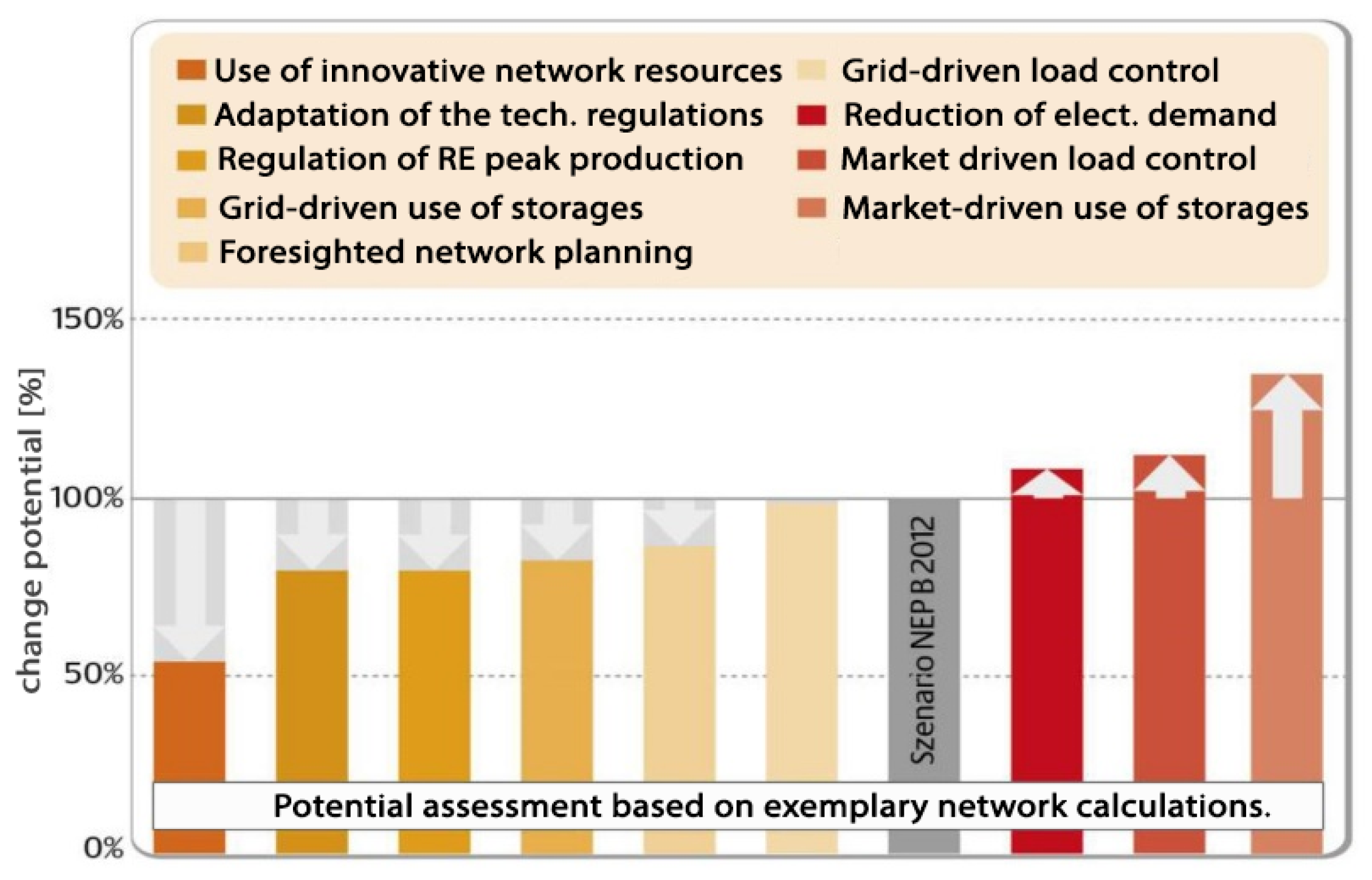
According to the EEG 2023, 80% of the electricity supply shall come from renewable energies by the year 2030. Assuming further electrification of transport, heat, and industrial processes will result in an annual energy demand of up to 600 TWh. To achieve this, energy generation from PV plants is to be increased to 215 GW, onshore wind plants to 115 GW, and offshore wind plants to 30 GW [4]. To reach these goals, the grids must be expanded in the first place. However, methods must also be developed to ensure the stability of the grids in the face of numerous volatile generators. Several scenarios for a possible grid expansion were simulated in the dena distribution grid study [5]. In the process, further-reaching measures and their effects on grid expansion costs were also examined (see Figure 1). “In the potential assessment, only the impact on the grid investment requirement was determined. Additional expenses, for example, for maintenance, operation, or the construction of storage facilities, were not taken into account. It should also be noted that the potentials of the individual options cannot be added together” [5]. This means that, in all scenarios, the avoided investment costs could be compensated or even exceeded by the additional operating costs. In addition to grid expansion, various control and optimisation methods were also examined.

Figure 1.
Variant calculation for different technical options in the electricity distribution grids until 2030 [5].
2.3. Grid Stability with Increased Use of Distributed Energy Systems
With the increase of renewable energy systems, the number of inverter systems connected to the grid also increases, which leads to a reduction of the grid quality due to the increased harmonic components, as already mentioned in the introduction. One of the reasons for this is the non-constant grid impedance. On the one hand, it depends on the node under test and the equipment connected to it. On the other hand, the equipment and the capacitance and inductance within it are also responsible for the fact that the network impedance is also frequency-dependent. Finally, it is also dependent on the connected loads and generation plants and their working points. Finally, the changing grid impedance is responsible for the fact that the filter resonance frequencies of the inverter systems shift and, thus, the grid disturbances become larger and thus the grid quality decreases [6,7]. According to [7], this can lead to serious effects up to the destruction of inverters or other plant components in weakly damped resonances between inverters and the grid or between several inverters.
According to [6], it can be assumed that problems with resonance points will tend to increase in the future as the proportion of capacitive elements in the grid increases. This is due to the increasing use of cables, and the resulting much higher operating capacity compared to overhead lines. The second trend is the increased use of power electronics and the associated filter circuits. For economic reasons, smaller coils and larger capacitors are increasingly being installed in these filters. These capacitors therefore also contribute to an increase in the capacitive component of the network impedance, which, in conjunction with the inductance of the network, leads to resonance points.
3. Algorithms for Load Flow Simulation
It is becoming apparent that the feed-in behaviour into the grids is becoming increasingly volatile, supported by various technologies with a wide variety of generation behaviour. Consumer behaviour is also changing, particularly influenced by electromobility and heat pumps. In order to prepare the energy grids for these requirements, a deeper understanding of the interactions between generation and consumption is needed, especially with regard to avoiding expansion efforts. This increases the necessity for simulations based on time series, which can span from 1 s up to several hours, depending on the requirements. The duration of the time series can ultimately be up to several years. Simulations over a whole year are certainly useful for examine the effects of the different seasons. Using the example of a time series over a year with a resolution of 10 s, this would mean that the simulation would have to be repeated 3,153,600 times. This can take up to several hours, depending on the degree of optimisation of the load flow program and algorithms used. Time series smaller than 1 s are also possible, but it has been shown that the static network behaviour can be simulated sufficiently accurately here. More precise simulations, such as those required for recording the network quality, should be carried out dynamically in the time domain. Simulations in the state-space offer good prerequisites for being able to carry out both time series simulations and dynamic simulations with effective values (RMS) and transient values (EMT) in real time. In comparison to common solution algorithms, the load flow simulation in the state-space shows the potential for speed optimisation, as will be shown below [8].
3.1. Mathematical Models Using an Admittance Matrix
A variety of methods for solving load flow problems can be found in the literature. The most common systems are the current iteration and the Newton–Raphson method, which are used to solve mathematical network models with an admittance matrix.
3.1.1. Setting up the Equation System
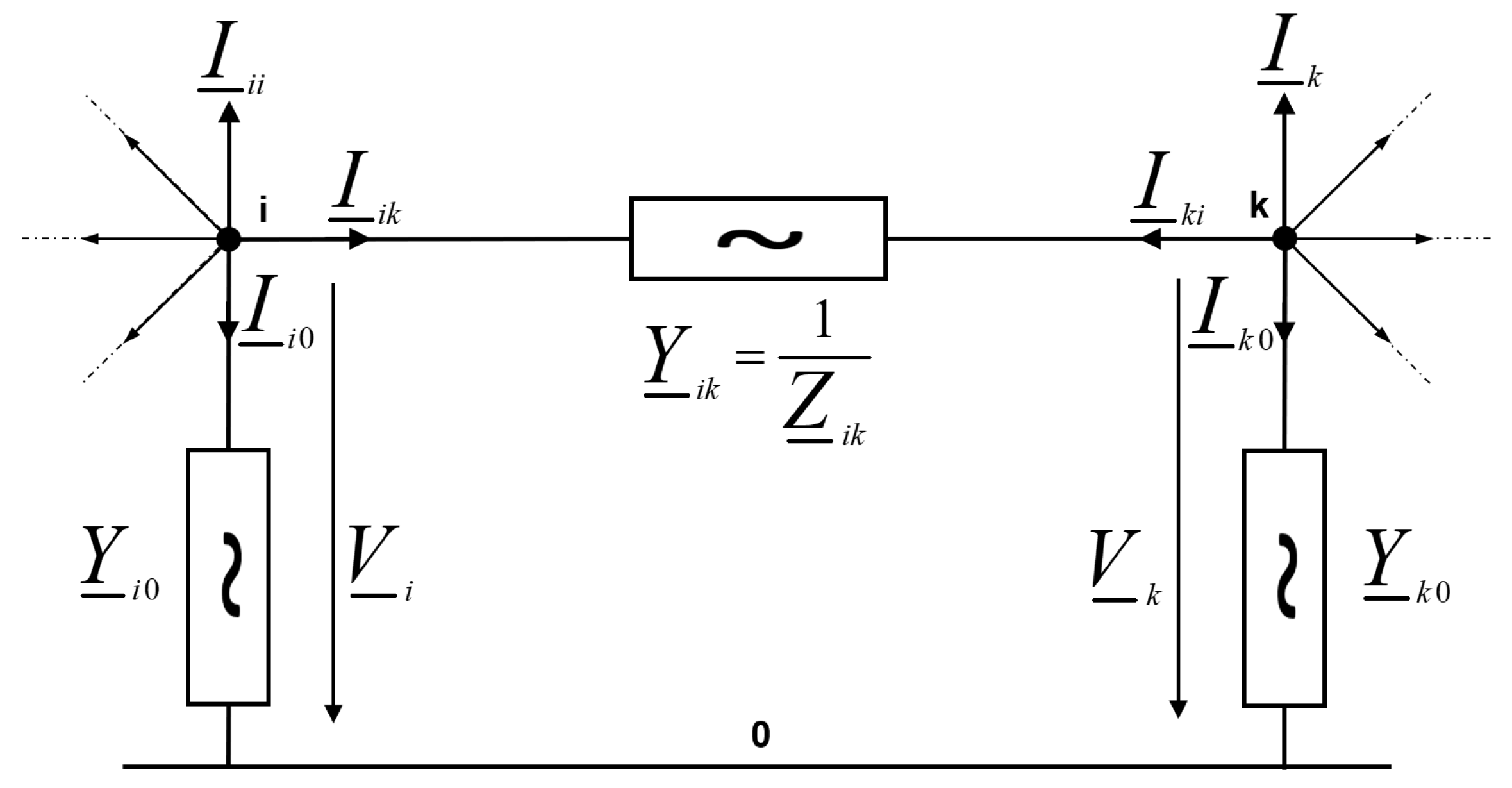
To set up the admittance matrix according to the node voltage method, all operating impedances of the network representation must be converted into admittances. In the single-phase network of Figure 2, the neutral conductor (N) is numbered 0, while all other nodes are numbered from 1 to n. The elements of the admittance matrix are calculated using the node voltage method. The network contains n + 1 nodes including the neutral conductor (N). In addition, an arbitrary reference point is chosen, which must neither be part of the network nor connected to it via passive components, e.g., a local earth electrode. Each node is assigned a node voltage which is referenced to the selected reference point. The current flowing from each node is positively registered and can be expressed by the node voltages at both ends of the current path and the admittance in between [9].
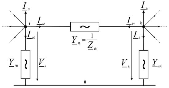
Figure 2.
Creating the admittance matrix using the example of a mesh with the nodes i and k.
When using the node voltage method, it is advantageous to use PI equivalent circuits to replicate passive equipment (transmission lines and transformers) instead of T equivalent circuits. This avoids the formation of additional nodes, which would increase the order of the equation system [10].
By applying Kirchhoff’s second law, the node current for each node can be calculated as follows:
The current flowing through the branches of the network can be calculated as shown in (2)
In summary, the current of each node can be expressed as a function of the voltages of the neighbouring nodes and the corresponding admittances of the branches, as shown in (3). This principle can be applied to all nodes of the network and used to set up a system of equations describing the node currents.
stands for the square admittance matrix, represents the vector of node voltages and the vector of node currents [9]. If there is no connection between two nodes, the corresponding element in the admittance matrix is zero [10]. Equation (5) applies to the admittance matrix formed in this way.
If the condition shown in (5) is fulfilled, this means that the system of equations cannot be solved uniquely. However, this can be worked around by choosing a suitable reference node (e.g., node 0 in Figure 2) and reducing the system of equations so that it transformed from a singular to a regular matrix. Unfortunately, this procedure often leads to ill-conditioned matrices. Nevertheless, the system can be further reduced by choosing another, arbitrary node as a constant-voltage node, so that it becomes solvable. In (6), this was achieved by using node 0 as the reference node and node 1 as the constant-voltage node [9].
The solvability of the equation system can be guaranteed by implementing the algorithms mentioned above.
3.1.2. Current Iteration Method
The current iteration method is a simple algorithm that determines the load flow of the system with a desired accuracy by including the specified node powers using iterative calculations of the corresponding currents and voltages of each node [2]. The node current can be calculated by dividing the complex conjugate apparent power and voltage at each node.
Furthermore, an improved node voltage can be determined iteratively for each iteration step via (4) [2]. When additionally considering the slack node (balance node), the equation system expands to
The equation system in (8) can be solved with the Jacobi method (total step method) as shown in (9).
Alternatively, the same can be achieved with the Gauss–Seidel method (one-step method), which is shown in (10).
With the one-step method, the improved node voltages of the previous iterations are taken into account in the calculation of the subsequent iterations. This leads to faster convergence.
However, generators have not been included in Equation (9) or Equation (10) until now. Unlike loads, a generator tries to adjust its node voltage to the generator nominal voltage at a given nominal active power . Since it can be assumed that the newly calculated voltages deviate from , a correction step must be carried out to correct it. For this, Equation (8) is extended to (11), whereby the nodes are separated into load (l) and generator (g) quantities [9].
For the correction of the node voltage, the absolute value of the node voltage is first set to the nominal generator voltage. For the angle, it is assumed that the calculated generator angle corresponds to a better approximation. Thus, the new node voltage at the generator results in
Since the voltage changed in this way also has an effect on the neighbouring nodes, these must also be corrected according to (13).
Finally, from the results obtained this way, the new reactive powers of the generators can be calculated according to (14).
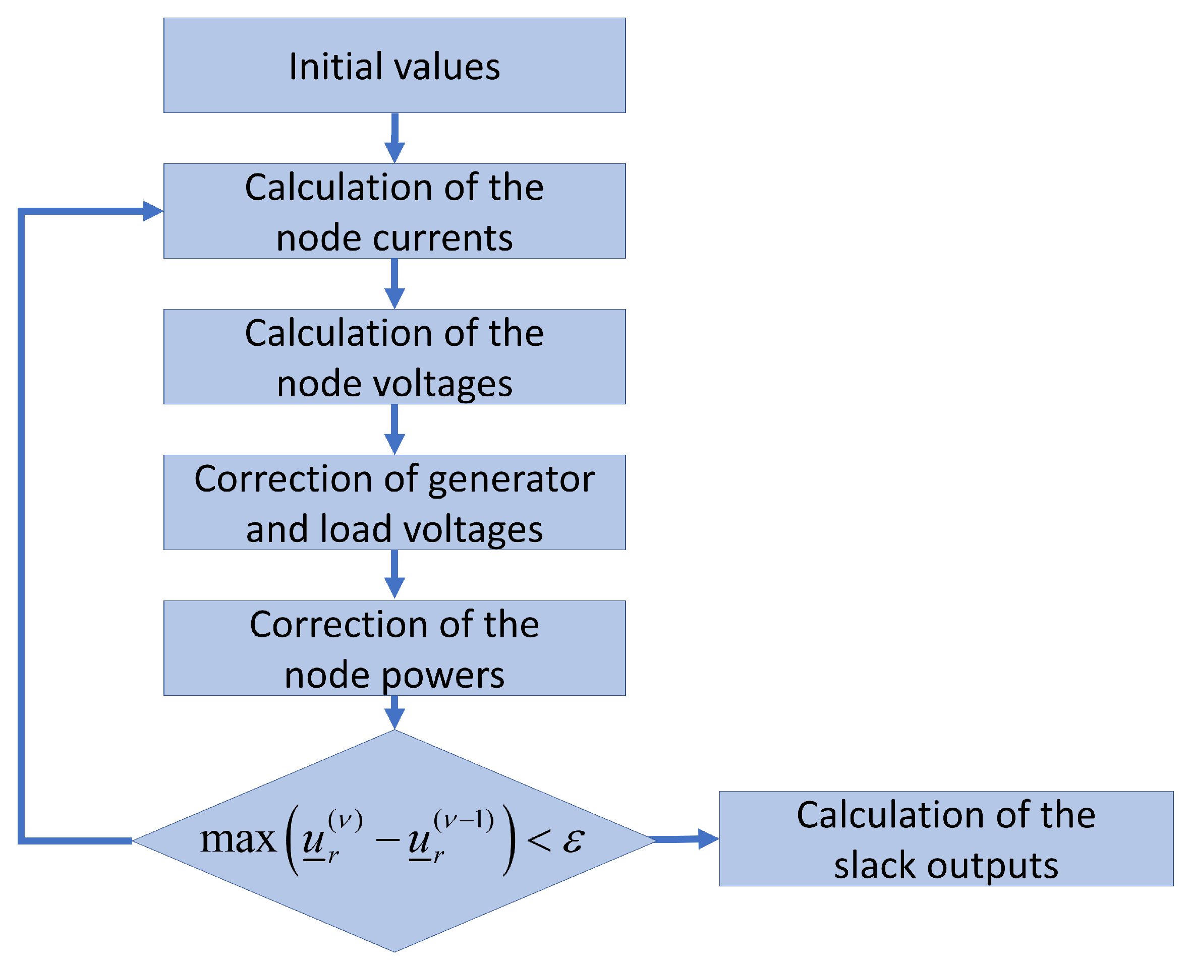
The new results for the voltages and powers can now be inserted back into Equations (9) and (10), respectively. The iteration is stopped when the desired accuracy is reached. Both the voltage change and the power deviation (the deviation of the calculated power from the nominal power ) can be used as termination criteria, as shown in (15) and (16) [11]. The entire procedure can be taken from Figure 3.
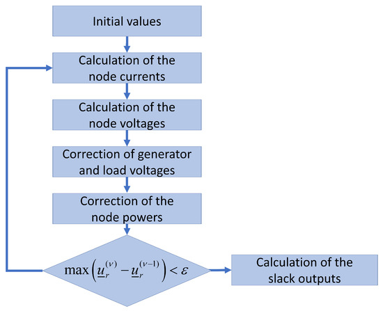
Figure 3.
Flowchart of the solver algorithm for the current iteration method.
The most important properties of the current iteration method are:
- Low convergence speed, i.e., many iterations are required until a sufficiently accurate solution is found;
- The number of iterations required depends on the network size and increases with the number of nodes;
- The inclusion of generator nodes is complex;
- High radius of convergence; even a poor initial prediction leads to a solution;
- Easy to program;
- Constant system matrix, which, unlike each iteration step, only needs to be built or inverted once.
Particularly in large networks, current iteration has convergence problems, so it is generally used less often today. Instead, the Newton–Raphson method is used [11].
3.1.3. Newton-Raphson Method
Newton’s method allows the approximation of non-linear functions with several variables. In the case of power flow analysis, these variables are represented by the equations for the node powers, which depend on the voltages applied to each node.
In general, the following applies to the active and reactive power at each node.
with
The previous equations apply for , since represents the slack node. To be able to solve these non-linear functions, they are expanded in a Taylor series, which is terminated after the first derivative (22). This transforms the non-linear load flow equations into a linear system of equations. The following recursion formula can be derived from the Taylor series, which is set up around an operating point .
This concept is applied to the equations for active and reactive power. The start vector is used for the expansion of the Taylor series.
The deviation between the calculated and the specified active and apparent power of each node for the selected starting vector is shown in (25) and (26).
The count variable is used to specify the iteration step of the recursion process. Applying all the previous steps for each node of the network leads to the system of equations in (27a), respectively (27b).
If there are generator nodes in (27a), due to the condition that the generator voltage is constant, the corresponding line in the lower section can be deleted and the condition can be set up.
In (27b), is the vector of the power deviations , is the vector of the deviations of the node voltages and , the so-called Jacobian matrix, which can also be represented as follows:
The diagonal and non-diagonal elements of the submatrix of the Jacobi matrix are calculated as follows [12]:
The diagonal and non-diagonal elements of the submatrix of the Jacobi matrix are calculated as follows:
The diagonal and non-diagonal elements of the submatrix of the Jacobi matrix are calculated as follows:
The diagonal and non-diagonal elements of the submatrix of the Jacobi matrix are calculated as follows:
Solving the load flow problem with the Newton–Raphson method requires several steps. First, assumptions are made about the initial conditions of the variables U and . The nominal voltages of the nodes with a phase shift of 0° are often suitable for this (the so-called flat start). The following steps are repeated iteratively until the power deviations and are smaller than a predefined accuracy . One of these steps to be repeated is the calculation of the active and reactive power of the nodes, as shown in (20) and (21). The results are used in (25) and (26) to calculate the power deviations of the individual nodes. If the desired accuracy has not been achieved, the voltage deviation is calculated by transforming (27b) as follows:
The node voltages are corrected and used to calculate the improved node performances of the next iteration. This process is repeated until the desired accuracy is achieved [10,12,13]. The entire process can be seen in Figure 4.
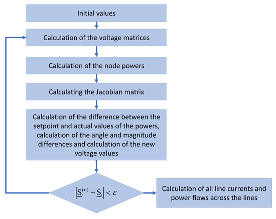
Figure 4.
Flowchart of the solver algorithm for the Newton–Raphson method.
The most important features of the Newton–Raphson method are:
- Complex programme structure;
- System matrices are usually highly overdefined. A network with N nodes has 2(N − 1) equations;
- Iterative recalculation of the Jacobian matrix required after each iteration step (very complex and time-consuming);
- Bad starting conditions can make convergence impossible;
- Fast iteration (approx. 3 …5 steps);
- Number of iterations is independent of the system size.
The equations shown above can also be set up in Cartesian form but the integration of the generator nodes, similar to the current iteration, is somewhat more complex, since the node voltages must be corrected here as well. However, the Newton–Raphson method in the Cartesian representation offers the following advantages [11]:
- The Jacobian matrix is easier to set up;
- The gradients of quadratic instead of trigonometric functions can be formed;
- The radius of convergence is larger.
3.2. State Space Modelling and Analytical Solution Methods
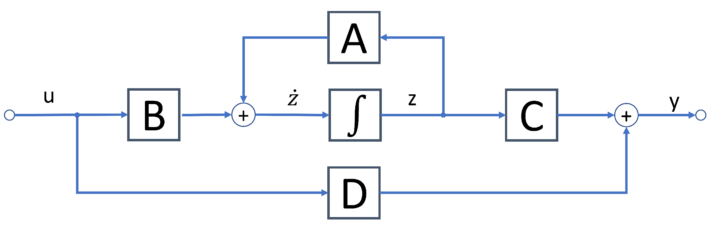
First, the network to be analysed is translated into the state-space by setting up the system’s corresponding network and node equations. This process is more complex than setting up the admittance matrix. First, the complete tree of the network must be established, upon which the state variables and the system matrices are obtained according to Figure 5. This process can be carried out with fundamental network analysis methods, such as those described here [14] or here [15].
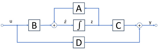
Figure 5.
Signal flow diagram of the state equations. It illustrates the relationship between the signal input and output vectors, the internal states z, as well as the system matrices A to D.
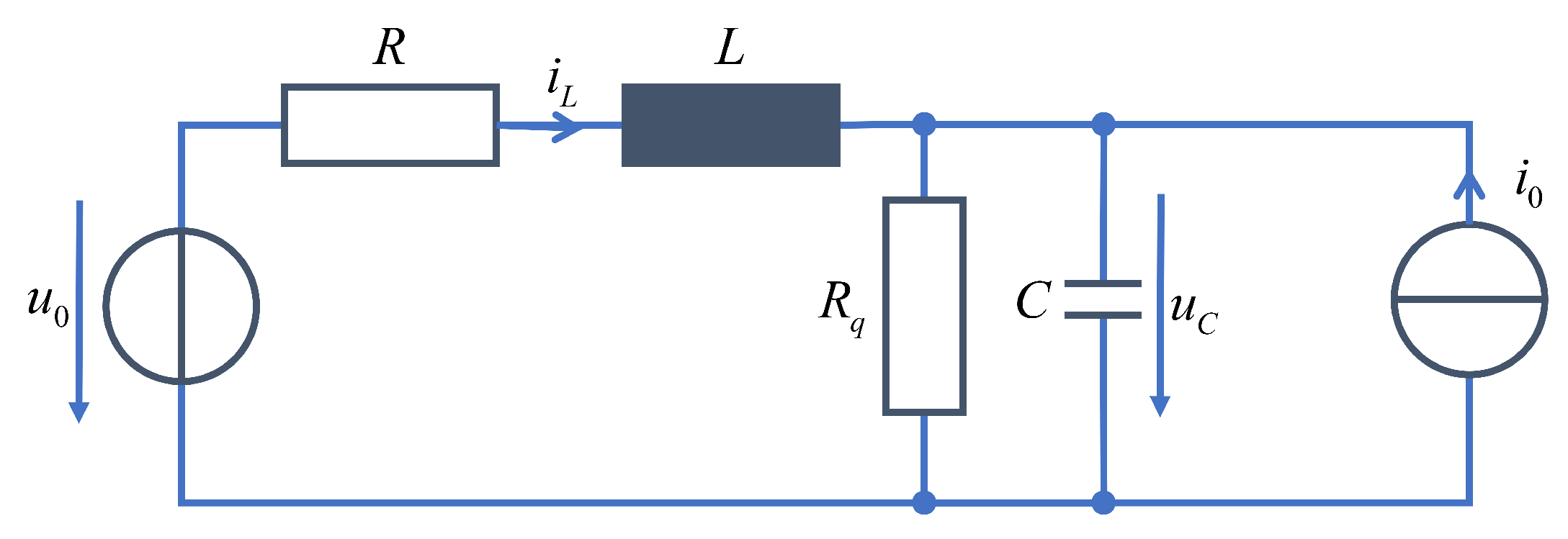
For very simple systems, such as those shown in Figure 6, the derivation of the corresponding differential equation system can be easily performed by hand. Under the premise that the energy stores in the system are linearly independent, the order of the differential equation system is equal to the number of energy stores. In most electrical power systems, at least some of the energy storage devices are interdependent. Therefore, the physically exact and necessary system representation can be derived by reducing the system to the rank of the analysed network. In this way, the system model becomes analytically solvable and minimal simulation times are obtained. By applying a systematic mathematical approach, the generation of system matrices in their minimal form is ensured and can be automated.
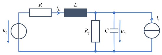
Figure 6.
Simple example system to illustrate the derivation process of the resulting differential equation system (energy storage: L, C—state variables: , ).
Furthermore, the derivation of the state space equations is realised in symbolic form, which enables the variation of system parameters without having to rebuild the system matrices for each time step. The basic principle of the methodology is explained below using the very simple example network shown in Figure 6.
Using Kirchhoff’s laws, a network analysis leads to the following differential equations:
which are used to set up the corresponding systems of equations. All impedances are normalised to the fundamental frequency . Therefore, the time variable is formally extended by the fundamental frequency,
This system description can also be represented in matrix notation as follows:
To solve this system, the implicit system representation from (37) can be converted into the explicit system representation (38) by means of a coefficient comparison.
where
This is the standard form for the differential equation system. Applied to Equation (37), according to [16], one obtains
With the help of the differential equations from (39) and suitable solution algorithms (e.g., Runge–Kutta method, Adams–Moulton method, Adams–Bashforth method, etc.), the system states of the given network can be calculated in the time domain in order to be able to simulate, e.g., transient or switch-on processes.
If these equations are transferred with
to calculate the load flow in the stationary (steady-state) operating case resulting from the mains-frequency supply, the solution of the system of equations can be further simplified. The time-dependent solution is thus transferred to a complex system of equations:
The matrices and represent the system impedances, the unit matrix, the vector of the sources, and the vector of the state variables of the system. This also makes it possible to analyse the frequency behaviour of the circuit, as is necessary, for example, for the harmonic analysis of frequency converters.
With Equation (41), it is also possible to perform load flow simulations in the state-space. In the undisturbed case, it can be assumed that and, therefore, applies. This simplifies the equation to
Assuming that the impedances of the system do not change due to, e.g., switching operations, it is possible to solve the load flow equation with only one mathematical operation for each different load situation. As already mentioned, the vector contains all sources of the system and thus also all controlled systems according to (47) or (48), which can be solved iteratively, as also described on page 14. The termination condition is
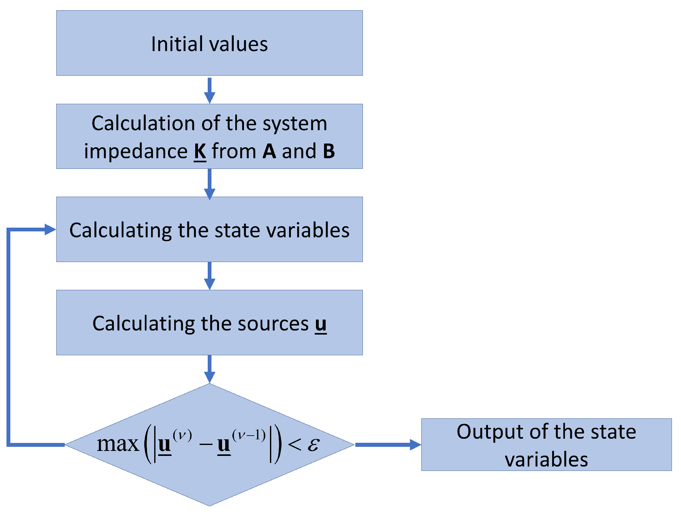
It is advantageous that the vector is set up in symbolic form, as this means that it does not have to be set up anew with each iteration, but only the new values have to be assigned to the corresponding variables. The sequence of the load flow simulation in the state-space is shown in Figure 7. It can be seen that only two calculation steps are necessary for the simulation. Without controlled systems, the entire calculation is even reduced to only one calculation run, which is less than with the other methods presented and is thus a possible alternative to shortening long time series calculations. With four to seven repetitions, the number of required iteration steps is also low.
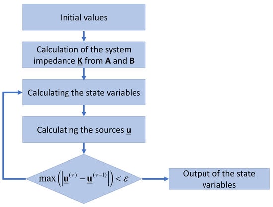
Figure 7.
Flowchart diagram of the solver algorithm for the load flow simulation in state-space.
The most important characteristics of the state-space method are:
- The state-space matrices provide a system representation of the physically minimum valid order;
- Direct system-theoretical solution of the load flow problem -> minimum of calculation operations and calculation times;
- Since the differential equation systems are available, it is possible to switch between static and transient simulations at any time without having to recalculate the system;
- Very good convergence properties;
- System matrices enable the implementation of control structures with increasing complexity (AI or agent system-based strategies for controlling smart grid systems, etc.).
4. Simulation of Basic Network Resources in State-Space
For the simulation of electrical networks in the state-space, a wide range of different components are required, whose physical properties should be simulated as realistically as possible. In order to be able to guarantee the greatest possible flexibility, all assemblies can be simulated in a specially developed program from the basic elements R, L, and C, the ideal transformer, as well as voltage and current sources. The four most important modules necessary for the load flow simulation are presented in the following.
4.1. Loads
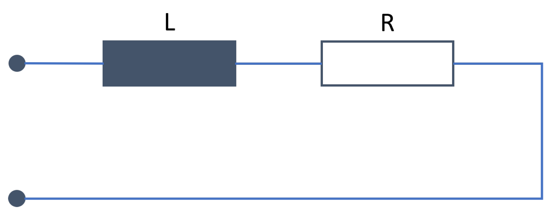
All loads are electrical energy converters that draw electrical energy from the grid. A distinction is made between regulated and unregulated loads or consumers with or without constant power consumption. Unregulated equipment generally does not have a constant power consumption, such as toasters or other heating systems, because their power consumption depends on their internal resistance and the grid voltage applied at the connection point (see also Figure 8).

Figure 8.
Simulation of a load, without regulation (simplified single-phase equivalent circuit).
Regulated loads, such as all modern switched-mode power supplies, on the other hand, can keep their power consumption constant over a wide voltage range, which can, however, also lead to increased load currents in mains areas with lower voltage. In both cases, the load can be simulated by an R-L element, through which the nominal power can be taken from the grid at nominal voltage.
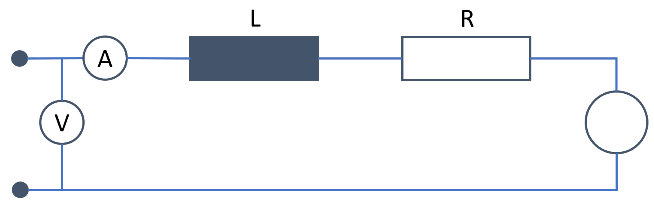
In order to be able to simulate a control system, a controllable source must be added to the circuit from Figure 8, as shown in Figure 9. The source can be either an ideal voltage or an ideal current source. Depending upon which type of source is chosen, different calculation methods result. The voltage and current meters represent the system variables needed for the calculation.
Figure 9.
Simulation of a controlled load (simplified single-phase equivalent circuit).
If the load is simulated via an ideal voltage source, the following formula results:
While choosing for the ideal current source, the equation is as follows:
In both equations, and are the predefined powers that are to be set at the load. Note that V can only be considered constant when the load is connected to a rigid source. In all other cases, it changes depending on the series resistor and load, which makes it necessary to solve the equations iteratively. Under this condition, Equations (45) and (46) result in:
where and where is the nominal voltage of the node and represents the iteration step, starting at 1. Comparing Equations (47) and (48), it is immediately apparent that loads with a constant current source should be preferred, as the resulting equations are less complex. In special constellations, however, it is necessary to use loads with voltage sources in order to be able to set up the equation system.
By varying the stored formulas, which influence the source currents or voltages, a wide variety of equipment can be simulated, from generators to power storage units, as the impressed currents can be both positive and negative.
4.2. Transformers
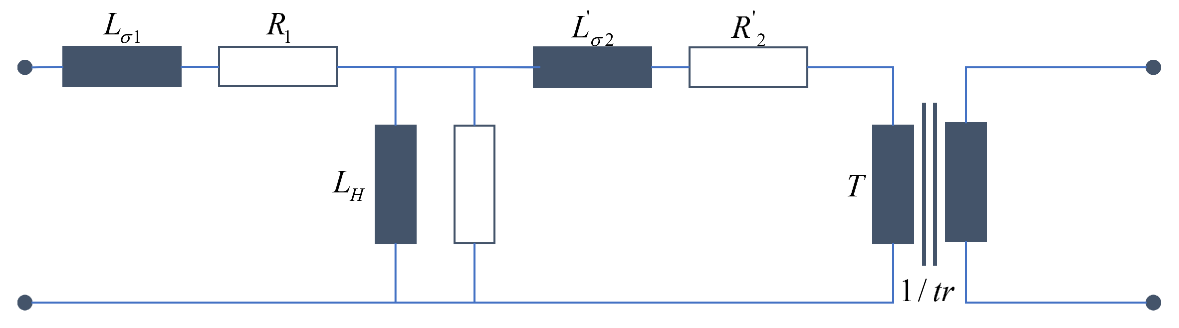
Transformers are essential for transmitting energy with as little loss as possible over long distances. Depending on the requirements, they can be constructed and internally connected in different ways. The single-phase equivalent circuit of a transformer according to Figure 10 takes into account the copper and stray losses of the primary side as well as the variables of the secondary side related to the primary side, as well as the core losses and the transformation ratio.
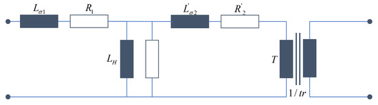
Figure 10.
Single-phase equivalent circuit diagram of a transformer.
The elements of the equivalent circuit can be determined from the real transformers’ short-circuit and open-circuit measurements. The copper and stray losses can be determined from the short-circuit measurements according to (49) and (50).
Here, is the nominal voltage on the primary side, is the referred short-circuit voltage in percent, is the referred ohmic short-circuit voltage in percent, and is the nominal apparent power of the transformer. Without further information, the short-circuit reactance can only be divided arbitrarily, since the currents of both windings are always involved in the leakage field. Usually, half of it is assigned to each winding [17]. Since the short-circuit resistances are often not measured separately, a similar approach must be taken here so that the following applies
From the open-circuit measurements, the elements of the cores can be calculated according to (53) and (54).
with
= Rated voltage of the secondary side (V)
= Iron losses (W)
= Referred open circuit current (%)
= Nominal apparent power of the transformer (VA).
The transmission ratio of the ideal transmitter T, which is still to be determined, is calculated from the nominal voltages as follows:
Here, is the phase shift of the secondary voltage to the primary voltage. It usually results automatically from the wiring of the transformer (see Section 4.4), but must be taken into account in the single-phase model.
4.3. Cables and Overhead Power Lines
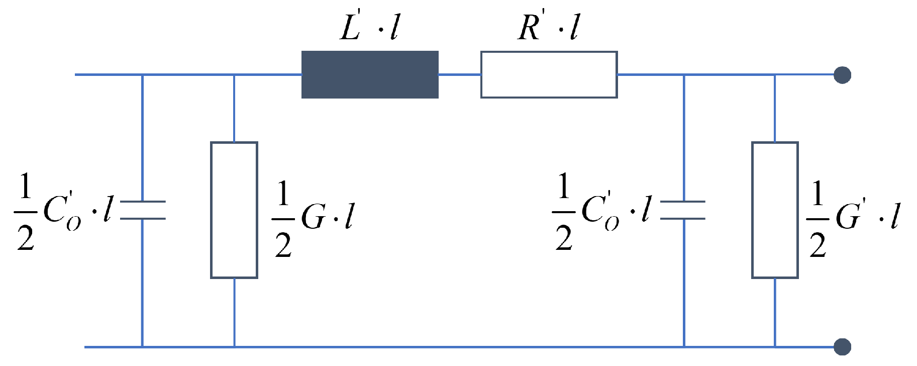
The overhead lines required for energy transmission can be generally simulated using the equivalent circuit diagram in Figure 11 for the case of a symmetrically constructed and operated system. The prerequisite here is that the line length l per element does not exceed 150 km, as otherwise distortions in the transfer function occur. However, long distances can be realised quite simply by connecting several elements in series. Only in the case of fast transient processes should the wave equations be used [2].

Figure 11.
Single-phase equivalent circuit diagram of an overhead line.
- with
= Resistance coating (/km);
= Inductance coating (H/km);
= Operating capacitance coating (F/km);
= Leakage coating (/km);
l = Length (km).
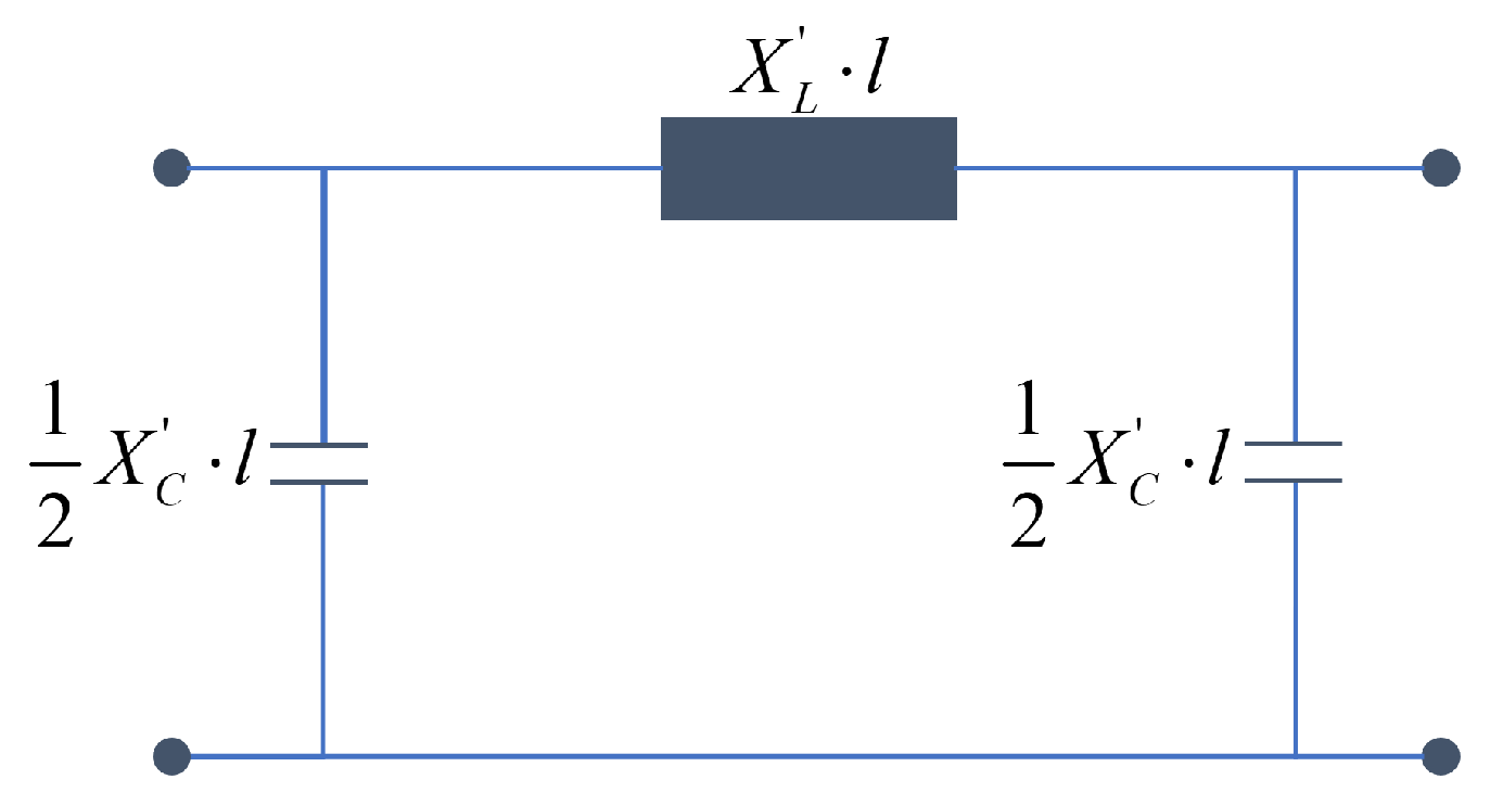
This equivalent circuit can be simplified in many cases. In the range of the grid frequency, usually applies for the transverse impedances, which is why the leakage resistance can be neglected. Assuming a steady state, the impedances can also be assumed at a constant angular frequency for a simpler simulation (here, ). For high-voltage cables, it can additionally be assumed that applies and thus the longitudinal reactance can be neglected, resulting in the equivalent circuit diagram according to Figure 12.
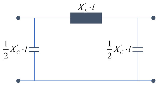
Figure 12.
Single-phase equivalent circuit diagram of a high-voltage overhead line.
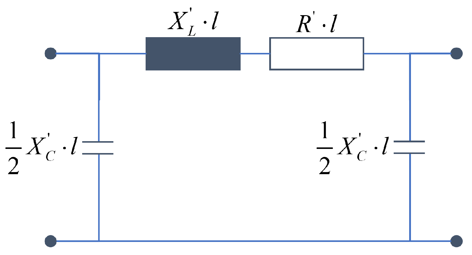
A simplified equivalent circuit can also be used for the medium-voltage and low-voltage overhead lines. Unlike with the high-voltage lines, however, the longitudinal reactances cannot be neglected here, but the operating capacity can, since this becomes much larger than the other elements due to the shorter distances. This results in the simplified equivalent circuit diagram in Figure 13.
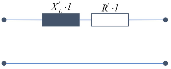
Figure 13.
Single-phase equivalent circuit diagram for an MV or LV overhead line or cable.
For cables, the corresponding parameters are determined differently than for overhead lines but a similar equivalent circuit results here as well. Only the leakage resistance is omitted here. Thus, medium-voltage cable results in a single-phase equivalent circuit as shown in Figure 14. For low-voltage cables, this equivalent circuit can also be simplified, since the operating capacitances can be neglected due to the low voltage. The corresponding equivalent circuit diagram can be seen in Figure 13 [2]. The values for the components can be taken from various cable manuals, e.g., [18].
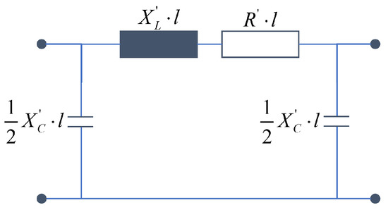
Figure 14.
Single-phase equivalent circuit diagram for a medium-voltage cable.
4.4. Symmetrical and Asymmetrical Simulation
In the case of an asymmetrical simulation, the procedure is the same as for a symmetrical simulation. In the asymmetrical simulation case, the single-phase models are replaced by three-phase models, effectively tripling the number of substitute elements, as shown in Figure 15.
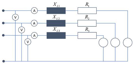
Figure 15.
Three-phase simulation of a PQ load for a state-space based simulation.
A great advantage of this type of modelling approach is the possibility of being able to replicate transformers correctly, merely by means of the wiring. The transformer in Figure 16 is simulated by three single-phase transformers (see Figure 10), which are connected accordingly. In this way, the desired behaviour is simulated without further intervention. Through the additional connections at the midpoint tap of the star side, a Dy5 and a Dyn5 can be simulated simultaneously with one model. The earth resistance can also be varied as desired.
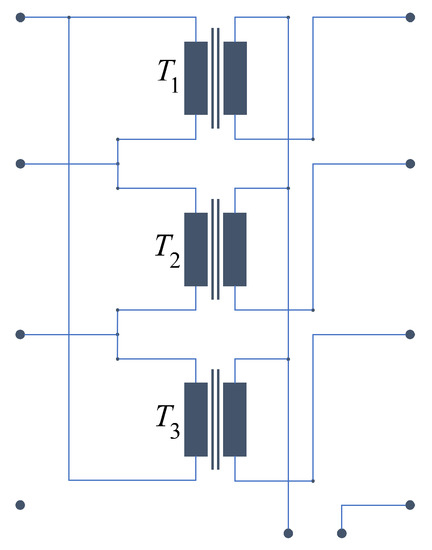
Figure 16.
Three-phase simulation model of a DY5(n) transformer.
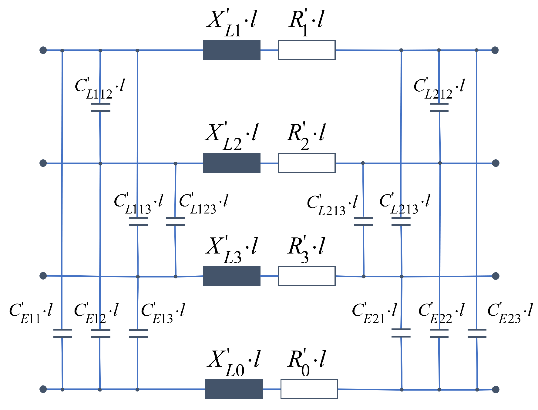
In overhead lines or cables, it is also possible to better represent capacitive and inductive couplings and the behaviour in the event of short circuits, for example. An example of a medium-voltage cable can be seen in Figure 17.
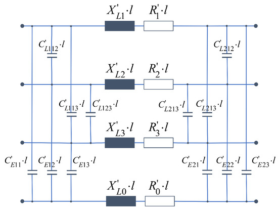
Figure 17.
Three-phase equivalent circuit diagram of a cable.
5. Comparison of Newton–Raphson Simulation and State-Space-Based Load Flow Calculation
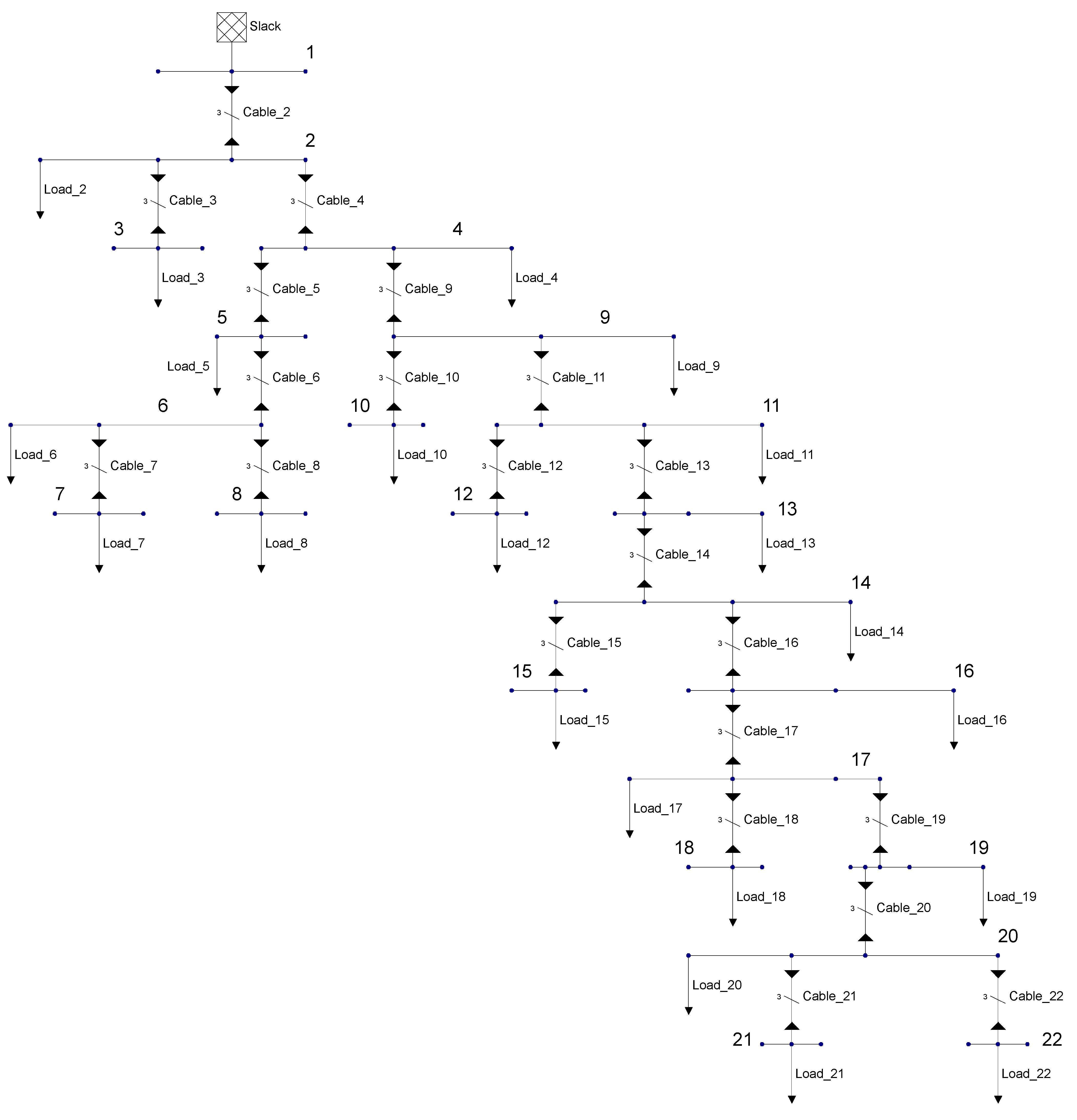
For the calculations of the load flow simulation in the state-space, a program was developed in Matlab, which carries out the required simulation steps. In order to compare the accuracy and speed of the simulation with the other two algorithms presented, MATPOWER [19], an open-source software based on various Matlab scripts, was used. As a test network, the case “case22” was selected, a system provided by MATPOWER based on [20]. This grid was also recreated for the StateSpace simulation in the Schematic Editor, a graphics editor developed specifically for this purpose (see Figure 18).
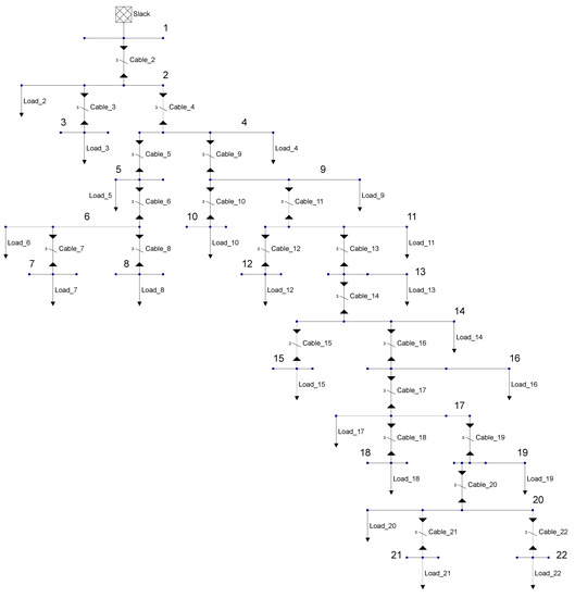
Figure 18.
Examined example network, based on [20].
For all three simulation methods, an accuracy of was chosen as the termination criterion. In order to be able to compare the results with each other, the differences of the calculated powers at the loads, between the programs and between the program results and the power setpoints were formed. The current iteration method could not be taken into account, as there was no convergence even after 500 iterations. The results of the remaining methods can be seen in Table 1. The precision with which the target output values are reached is clearly evident for both programs, thereby validating the state-space calculations. Furthermore, the largest voltage and power deviations amount to 2 nV, 67 nW, respectively. The scale of these results suggests that the deviations are negligible and can be disregarded without committing a significant error. The state-space method is able to achieve the aforementioned levels of accuracy after only a few iteration steps. However, there is still great potential for optimisation within the StateSpace program structure, which should enhance the simulation performance even further. A clear advantage for the method in the state-space is the possibility to seamlessly switch from the load flow simulation to a time domain simulation, which can definitely be advantageous for future requirements, whereby the load flow simulation in the state-space could establish itself as a good alternative.

Table 1.
Comparison of simulation results between the StateSpace and the Newton–Raphson algorithms.
6. Conclusions
The state-space-based load flow simulation approach represents a fast and efficient method of simulating the behaviour of power grids and power systems for varying operating conditions. In contrast to the other two methods presented, in state-space it is possible to solve networks without controlled systems directly on the basis of complex equation systems, whereas current iteration methods, as well as Newton–Raphson methods, are based on an iterative determination of all solutions. At the same time, the presented method has a fast convergence on networks with controlled, nonlinear loads and requires only a few iterations to find a precise solution. In contrast to the current iteration procedure, the convergence behaviour does not depend on the number of nodes (network size). Additionally, the method presented above also offers, due to its symbolic matrices and the exact and also quite simple algorithm, the possibility of additional flexibility and the simplification of the calculations because the system matrices had to be built up only once as long as the system structure remained unchanged. Of course, all system variables (e.g., impedance, voltages, currents, etc.) may vary. This can considerably increase the speed of the calculation and therefore also has an advantage over the Newton–Raphson method, in which the Jacobian matrix must be rebuilt for each iteration step. For time series simulations especially, the necessary simulation time can be effectively reduced. The calculations can be applied to complex networks with numerous nodes and links and can also be used for various operating conditions such as dynamic loads, network component failures, or power system disturbances, all of which can be realised using the same set of equivalent circuit models. It offers high accuracy as it can model a system’s behaviour by accounting for system dynamics, non-linear loads, and voltage harmonics, essentially providing very detailed information concerning the system’s performance. This also allows simulation of the frequency-dependent behaviour of inverters, either, as described in [7], via the corresponding Thévenin equivalent or by directly inserting the state-space models, as shown in [6]. The advantage of this method is to be able to first calculate the corresponding grid states via the load flow simulation and then simulate the dynamic behaviour of the inverters based on these operating points. This option is not, or not directly, available in many other simulation systems. However, since dynamic inverter models can become very complex, their useful application is to be limited to rather small networks in most cases. A detailed investigation is in prospect. Further investigations will focus on the integration of thermal networks via thermal-electric models. Good results have already been achieved in first tests. The design as an open system also offers the possibility of a direct implementation of a wide variety of regulatory control systems. A subordinate disadvantage of the developed method is that the derivation of the complete tree structure, which is necessary for establishing the system’s equations in state space, requires an increased computational effort compared to, e.g., the Newton–Raphson method. On the other hand, the system equations are available in minimal form, thus enabling an exact calculation of the system’s states in a minimal computation time. Only the physically necessary power controls have to be iteratively reproduced. All in all, the load flow simulation in the state-space offers many advantages that could be an interesting alternative to the conventional load flow calculation when it comes to simulating the complex, time series-based influences of modern power grids; this can be of increasing relevance in the future, especially in terms of the maintenance of the system stability under the future plans of the European government but also of the environmental protection concepts of other countries.
Author Contributions
Research T.B.; simulation, T.B.; evaluation and writing—original, T.B.; draft preparation, T.B., validation, T.B. and C.W.; Conceptualization, T.B.; writing—review and editing, C.W.; project administration, C.W.; funding acquisition, C.W. All authors have read and agreed to the published version of the manuscript.
Funding
This research was funded by the Federal Ministry for Economic Affairs and Climate Action. Grant number: 03El4027B. 
Data Availability Statement
All data used has been published here.
Conflicts of Interest
The authors declare no conflict of interest.
References
- Bundesnetzagentur für Elektrizität, Gas, Telekommunikation, Post und Eisenbahnen. Bericht zum Zustand und Ausbau der Verteilernetze 2021. Available online: https://www.bundesnetzagentur.de/SharedDocs/Downloads/DE/Sachgebiete/Energie/Unternehmen_Institutionen/NetzentwicklungUndSmartGrid/ZustandAusbauVerteilernetze2021.pdf?__blob=publicationFile&v=4 (accessed on 19 January 2023).
- Heuck, K.; Dettmann, K.D.; Schulz, D. Elektrische Energieversorgung; Vieweg+Teubner: Wiesbaden, Germany, 2010. [Google Scholar]
- Bundesnetzagentur und Bundeskartellamt Monitoringbericht 2022, Bonn, Germany, 2023. Available online: https://www.bundesnetzagentur.de/DE/Fachthemen/ElektrizitaetundGas/Monitoringberichte/start.html (accessed on 19 January 2023).
- Neuer Schwung für erneuerbare Energien, Berlin, Germany, 2022. Available online: https://www.bmwk.de/Redaktion/DE/Schlaglichter-der-Wirtschaftspolitik/2022/10/05-neuer-schwung-fuer-erneuerbare-energien.html (accessed on 19 January 2023).
- Höflich, B. Ergebniszusammenfassung der PSG zur dena-Verteilnetzstudie: Zusammenfassung der zentralen Ergebnisse der Studie “Ausbau- und Innovationsbedarf in den Stromverteilnetzen in Deutschland bis 2030” durch die Projektsteuergruppe. 2012. Available online: https://www.dena.de/fileadmin/dena/Dokumente/Pdf/9100_dena-Verteilnetzstudie_Abschlussbericht.pdf (accessed on 4 May 2023).
- Jessen, L. Untersuchung der Wechselwirkungen Zwischen Dezentralen Erzeugungsanlagen und Energieversorgungsnetzen. Ph.D. Thesis, Christian-Albrechts-Universität zu Kiel, Kiel, Germany, 2018. [Google Scholar]
- Rogalla, S.C. Analyse frequenzabhängiger Netzwechselwirkungen von selbstgeführten Wechselrichtern Mittels Differentieller Impedanzspektroskopie und Oberschwingungsquellenbetrachtung. Ph.D Thesis, Technische Universität Braunschweig, Braunschweig, Germany, 2020. [Google Scholar]
- Blenk, T.; Weindl, C. Characteristics and Advantages of a State-Space Orientated Calculation in Regenerative Energy Systems. In Proceedings of the 2022 IEEE International Conference on Diagnostics in Electrical Engineering (Diagnostika), Pilsen, Czech Republic, 6–8 September 2022; pp. 1–5. [Google Scholar] [CrossRef]
- Schwab, A.J. Elektroenergiesysteme; Springer: Berlin/Heidelberg, Germany, 2020. [Google Scholar] [CrossRef]
- Oeding, D.; Oswald, B.R. Elektrische Kraftwerke und Netze; Springer: Berlin/Heidelberg, Germany, 2016. [Google Scholar] [CrossRef]
- Wolter, M. “Elektrische Netze 1”: Stationäre und quasistationäre Netzberechnung, Magdeburg, Germany, 2020. Available online: https://www.lena.ovgu.de/lena_media/Dokumente+und+Skripte/Skript_EN1.pdf (accessed on 4 May 2022).
- Nirupama, S. Newton-Raphson Method to Solve Power Flow Problem: Electrical Engineering, 2021. Available online: https://www.engineeringenotes.com/electrical-engineering/power-flow/newton-raphson-method-to-solve-power-flow-problem-electrical-engineering/25354 (accessed on 10 January 2023).
- Schäfer, K.F. Netzberechnung; Springer: Wiesbaden, Germany, 2020. [Google Scholar] [CrossRef]
- Schneider, M.E. Stationäre Optimierung elektrischer Energieversorgungsnetze im Zustandsraum. Ph.D. Thesis, Friedrich-Alexander-Universität Erlangen-Nürnberg, Erlangen, Germany, 1999. [Google Scholar]
- Schwarz, R. Analyse Nichtlinearer Netzwerke im Erweiterten Zustandsraum; Grundlagen der Schaltungstechnik, Oldenbourg: München, Germany; Wien, Austria, 1989. [Google Scholar]
- Weindl, C.; Herold, G. Description of a State-Space Oriented Transient Network Simulation Methodology for Power Systems with Semiconductor Based Devices. Ph.D. Thesis, University of Erlangen-Nürnberg, Bavaria, Germany, 2004. [Google Scholar]
- Herold, G. Parameter Elektrischer Stromkreise—Leitungen—Transformatoren, 2nd ed.; Elektrische Energieversorgung/von Gerhard Herold; Schlembach: Wilburgstetten, Germany, 2008; Volume 2. [Google Scholar]
- Tabellen mit Projektierungsdaten für Kabel, Leitungen und Garnituren: Angaben zur Querschnittsbemessung, 4th ed.; Kabel und Leitungen für Starkstrom/Hrsg; Siemens-Aktienges: Berlin, Germany, 1989; Volume Teil 2.
- Zimmerman, R.D.; Murillo-Sánchez, C.E. MATPOWER, 2020. Available online: https://matpower.org/ (accessed on 19 January 2023). [CrossRef]
- Ramalinga Raju, M.; Ramachandra Murthy, K.; Ravindra, K. Direct search algorithm for capacitive compensation in radial distribution systems. Int. J. Electr. Power Energy Syst. 2012, 42, 24–30. [Google Scholar] [CrossRef]


Disclaimer/Publisher’s Note: The statements, opinions and data contained in all publications are solely those of the individual author(s) and contributor(s) and not of MDPI and/or the editor(s). MDPI and/or the editor(s) disclaim responsibility for any injury to people or property resulting from any ideas, methods, instructions or products referred to in the content. |
© 2023 by the authors. Licensee MDPI, Basel, Switzerland. This article is an open access article distributed under the terms and conditions of the Creative Commons Attribution (CC BY) license (https://creativecommons.org/licenses/by/4.0/).