Large Neighborhood Search for Electric Vehicle Fleet Scheduling

Abstract

This work considers the problem of planning how a fleet of shared electric vehicles is charged and used for serving a set of reservations. While exact approaches can be used to efficiently solve small to medium-sized instances of this problem, heuristic approaches have been demonstrated to be superior in larger instances. The present work proposes a large neighborhood search approach for solving this problem, which employs a mixed integer linear programming-based repair operator. Three variants of the approach using different destroy operators are evaluated on large instances of the problem. The experimental results show that the proposed approach significantly outperforms earlier state-of-the-art methods on this benchmark set by obtaining solutions with up to 8.5% better objective values.

1. Introduction

The electrification of mobility is seen as an important step towards a reduction in greenhouse gas emissions [1]. More specifically, the electrification of company car fleets is considered particularly beneficial since company cars have a higher annual mileage and a shorter ownership period compared to privately owned cars [2,3]. Compared to uncontrolled charging, a smart charging strategy [4] can not only help to reduce the cost of a fleet of electric vehicles (EVs) but also relieve the power grid [5]. The operator of an EV fleet might not only decide how the EVs are charged but also how they are used, i.e., which EV is used in which time period.

In the present paper, the problem of simultaneously planning the charging and usage of a fleet of shared EVs is considered. More precisely, a fleet of EVs, which are charged at a common site and a set of vehicle reservations is considered. The problem consists in optimizing the charging schedule of the EVs and the assignment of vehicle reservations to individual EVs in order to maximize the utilization of the EVs for serving reservations while keeping the charging cost low.

There are numerous works regarding the optimization of EV charging plans considering different objectives and constraints. For example, Jin et al. [6] consider the use of EVs for the provision of regulation services. Igualada et al. [7] describe how EV charging can be integrated into the management of a microgrid. Franco et al. [8] propose an approach for EV charging planning taking the stability of the distribution network into account. Naharudinsyah and Limmer [9] integrate trading on a real-time electricity market into the charging planning. Schaden et al. [10] consider in the charging planning that, especially for fast charging, the maximum charging power decreases nonlinearly with an increasing state of charge. In most works, linear programming or mixed integer linear programming (MILP) is employed for the optimization of EV charging plans.

Furthermore, there are a number of works that plan the use of EVs in terms of routes, including recharging operations along the routes [11]. Different exact approaches, such as branch-and-cut [12], branch-price-and-cut [13], and branch-and-cut supported by simulated annealing [14] as well as heuristic approaches such as the variable neighborhood search algorithm [15], adaptive large neighborhood search [16], and deterministic annealing [17] have been proposed for the EV routing problem.

As mentioned before, in the present work, the planning of reservation assignments instead of routes is considered. This problem was already investigated by Varga et al. [18]. They showed that a MILP approach can effectively solve the problem as long as the number of considered EVs and reservations is not too high but that this approach scales poorly with increasing problem size. The authors, therefore, proposed an improved exact approach based on Benders decomposition [19] supported by a heuristic and compared it to the standard MILP approach on problem instances with up to 100 EVs and 1600 reservations. Later, Limmer et al. [20] proposed a hybrid evolutionary approach for the EV fleet scheduling problem, where the assignment of EVs to reservations is optimized with an evolutionary algorithm, and in the fitness evaluation, linear programming is used to optimize a charging plan for the fixed reservation assignment. Furthermore, the authors described two surrogate-based variants of the approach. Experiments on some of the largest problem instances considered in [18] showed that the proposed evolutionary approach—especially the surrogate-based variants—notably outperforms the standard MILP approach, as well as the Benders decomposition approach from, [18] on these problem instances from a heuristic perspective. In earlier works, Betz et al. [21] proposed a MILP approach and Sassi and Oulamara [22] proposed a problem-specific heuristic for the EV fleet scheduling problem. However, these works considered problem variants other than the variant considered in the present work and the proposed approaches are not directly applicable to the problem variant considered here.

In this work, a large neighborhood search (LNS) [23] approach is proposed for the EV fleet scheduling problem. LNS is a popular heuristic for combinatorial optimization problems. It traverses the search space by iteratively destroying and repairing parts of the so-far best-found solution. LNS has been successfully applied to different problems such as vehicle routing [24], job scheduling [25], and placement of service points [26]. The proposed LNS employs a MILP-based repair operator. The approach is evaluated and compared to earlier approaches in experiments on the problem instances from [20]. In order to investigate the effect of the employed destroy operator on the performance of the proposed approach, three different destroy operators are considered in the experiments. The experimental results show that the proposed approach significantly outperforms earlier methods.

The rest of the paper is structured as follows: Section 2 describes the considered problem in detail. In Section 3, the LNS is explained. Section 4 describes the setup of the experiments and presents and discusses obtained results. Finally, Section 5 provides a summary and draws conclusions.

2. Problem Description

The problem consists in planning the charging and usage of a homogeneous fleet $\mathcal{N}=\{1,\cdots ,N\}$ of N EVs over a planning horizon $\mathcal{T}=\{1,\cdots ,T\}$ of T discrete time steps of length $\Delta t$. Each EV $n\in \mathcal{N}$ can be charged with a maximum power of $P^{\max }$ kW, has a battery capacity of $E^{\max }$ kWh, and has a certain initial battery level of $E_n^{\mathrm{init}}$ kWh at the beginning of the planning horizon. The EVs can be charged at a common site with a certain electrical base load and photovoltaic (PV) energy production. In time steps t with PV overproduction, the corresponding surplus energy $Su{r}_t$ can be used for charging the EVs. Let $Su{r}_t$ be zero for time steps t without overproduction. Additionally to surplus energy, energy from the power grid can be used for EV charging, where time-varying prices have to be paid for the grid energy. Let $p_t$ denote the energy price in monetary units per kWh in time step t. Concerning the usage of the vehicle fleet, a set $\mathcal{R}=\{1,\cdots ,R\}$ of R vehicle reservations is given. Each reservation $r\in \mathcal{R}$ requests an arbitrary vehicle for a time period starting with a certain time step $t_r^s\in \mathcal{T}$ and ending with a certain time step $t_r^e\in \mathcal{T}$. The usage of an EV for serving a reservation $r\in \mathcal{R}$ is assumed to consume a certain amount $E_r^{\mathrm{res}}$ of energy.

The charging of the EVs in conjunction with the assignment of EVs to reservations should be optimized according to the following formal model:

$$min\alpha {\displaystyle \sum _{r\in \mathcal{R}}}{E}_r^{\mathrm{res}}·y_r+{\displaystyle \sum _{t\in \mathcal{T}}}{p}_t·E_t^{\mathrm{grid}}+\beta {\displaystyle \sum _{n\in \mathcal{N}}}\left(E^{max}-E_{n,T}\right),$$

(1)

subject to

${\displaystyle \sum _{n\in \mathcal{N}}}{x}_{n,r}+y_r=1$	$\forall r\in \mathcal{R},$	(2)
$P_{n,t}\le P^{\max }·(1-{\displaystyle \sum _{r\in \mathcal{R}|t_r^s\le t\le t_r^e}}{x}_{n,r})$	$\forall n\in \mathcal{N},\forall t\in \mathcal{T},$	(3)
$E_{n,1}=E_n^{\mathrm{init}}+\Delta t·P_{n,1}-{\displaystyle \sum _{r\in \mathcal{R}|t_r^s=1}}{x}_{n,r}·E_r^{\mathrm{res}}$	$\forall n\in \mathcal{N},$	(4)
$E_{n,t}=E_{n,t-1}+\Delta t·P_{n,t}-{\displaystyle \sum _{r\in \mathcal{R}|t_r^s=t}}{x}_{n,r}·E_r^{\mathrm{res}}$	$\forall n\in \mathcal{N},\forall t\in \mathcal{T}\setminus \left\{1\right\},$	(5)
${\displaystyle \sum _{n\in \mathcal{N}}}\Delta t·P_{n,t}=E_t^{\mathrm{grid}}+E_t^{\mathrm{sur}}$	$\forall t\in \mathcal{T},$	(6)
$0\le P_{n,t}\le P^{\max }$	$\forall n\in \mathcal{N},\forall t\in \mathcal{T},$	(7)
$0\le E_{n,t}\le E^{\max }$	$\forall n\in \mathcal{N},\forall t\in \mathcal{T},$	(8)
$0\le E_t^{\mathrm{grid}}$	$\forall t\in \mathcal{T},$	(9)
$0\le E_t^{\mathrm{sur}}\le Su{r}_t$	$\forall t\in \mathcal{T},$	(10)
$x_{n,r}\in \{0,1\},y_r\in \{0,1\}$	$\forall n\in \mathcal{N},\forall r\in \mathcal{R}.$	(11)

Binary variables $x_{n,r}$ indicate whether a reservation r is assigned to EV n. Note that not all reservations need to be assigned to an EV. Unassigned reservations are indicated by binary variables $y_r$, and they are, for example, served by rented or remaining combustion engine cars. Variables $P_{n,t}$ reflect the charging powers for each EV n in each time step t. Moreover, variables $E_t^{\mathrm{grid}}$ and $E_t^{\mathrm{sur}}$ denote the amount of grid and surplus energy, respectively, used for EV charging in time step t. Last but not least, variables $E_{n,t}$ denote the battery levels of each EV n in each time step t. The objective function (1) is a weighted sum of three sub-objectives: The first term minimizes the amount of energy corresponding to unassigned reservations, which is equivalent to maximizing the amount of used energy covered by EVs. The second term minimizes the energy cost. Finally, the third term maximizes the battery levels of the EVs at the end of the planning horizon in order to increase the chances that reservations arriving in the future can be served by EVs. Constraints (2) ensure that each reservation r is either assigned to an EV or $y_r$ is set to one. Constraints (3) ensure that an EV is not charged in time steps in which it is used for a reservation; moreover, they prevent an EV from being assigned to two reservations overlapping in time. Constraints (4) and (5) set the battery levels of the EVs in the first and the following time steps, respectively. Lastly, Constraints (6) ensure the energy balance.

3. LNS Approach

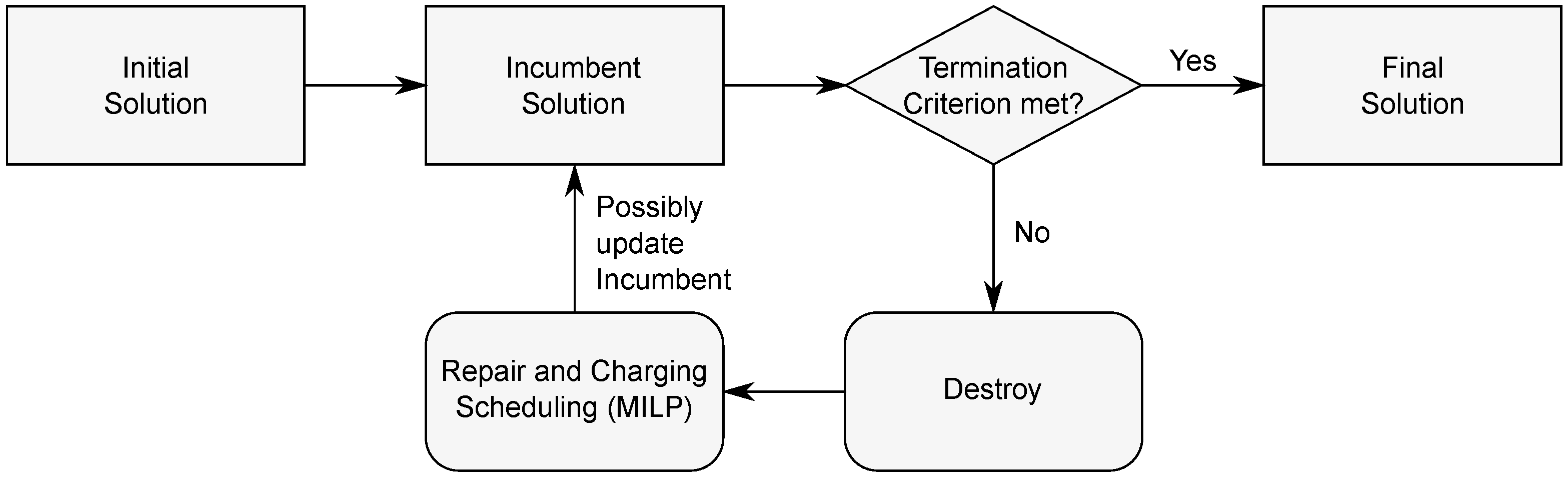
Large neighborhood search is a popular destroy-and-repair heuristic. Starting from an initial solution, it iteratively destroys a part of the currently best solution and repairs it. If the resulting solution is better than the currently best solution, the currently best solution is updated; otherwise, the resulting solution is rejected. The workflow of the employed LNS is illustrated in Figure 1 and outlined in Algorithm 1. In the following, the used operations are explained in detail.

Algorithm 1: LNS Approach

3.1. Initialization

The LNS starts with computing for each reservation $r\in \mathcal{R}$ the energy consumption $e_r=\frac{E_r}{t_r^e-t_r^s+1}$ per time step of its duration and sorting the reservations in non-increasing order of their respective $e_r$ values. The sorted reservations are then passed to a basic insertion operator in order to compute an initial solution, which is outlined in Algorithm 2. Reservation assignments are encoded as a list $A=[A_1,\cdots ,A_N]$ of N lists, where $A_n$ contains the reservations assigned to vehicle n for $n=1,\cdots ,N$. The basic insertion operator starts with an empty reservation assignment. It then iterates over the reservations in their passed order, and for each reservation r, it iterates over the EVs and adds r to the reservation assignments of the first EV for which the resulting reservation assignment is feasible. A reservation assignment of an EV is feasible if the assigned reservations do not overlap in time and there is a charging schedule that allows the EV to satisfy the energy requirements of the assigned reservations. The latter can be determined by simply evaluating whether the energy requirements are satisfied if the EV is charged uncontrolled, i.e., with maximum possible charging power, in all time steps in which it is not used for a reservation. The basic insertion operator returns the resulting reservation assignment and the reservations it could not assign. The order in which reservations are passed to the insertion operator has a major impact on the result. In particular, reservations at the beginning of the passed list have a higher chance to be assigned to an EV than reservations at the end of the passed list. This is the reason why reservations are passed in decreasing order of their energy consumption per time step of duration. Assigning a reservation with a high energy consumption contributes much to the first term of the objective function (1) and a short duration increases the chance that further reservations can be assigned.

Algorithm 2: Basic insertion operator

3.2. Evaluation

After an initial solution has been determined by the basic insertion, the LNS computes its objective value. In order to compute the second and third term of the objective function, the charging of the EVs has to be scheduled. This is performed by optimizing the charging schedule with linear programming (LP) for the reservation assignment as encoded in the solution. More precisely, the following optimization problem is solved:

$$\begin{array}{c}min{\displaystyle \sum _{t\in \mathcal{T}}}{p}_t·E_t^{grid}+\beta {\displaystyle \sum _{n\in \mathcal{N}}}(E^{max}-E_{n,T}),\end{array}$$

(12)

subject to:

$E_{n,1}=E_n^{init}+\Delta t·P_{n,1}-{\displaystyle \sum _{r\in {\mathcal{A}}_n|t_r^s=1}}{E}_r^{res}$	$\forall n\in \mathcal{N},$	(13)
$E_{n,t}=E_{n,t-1}+\Delta t·P_{n,t}-{\displaystyle \sum _{r\in {\mathcal{A}}_n|t_r^s\le t}}{E}_r^{res}$	$\forall n\in \mathcal{N},\forall t\in \mathcal{T}\setminus \left\{1\right\},$	(14)
${\displaystyle \sum _{n\in \mathcal{N}}}\Delta t·P_{n,t}=E_t^{grid}+E_t^{sur}$	$\forall t\in \mathcal{T},$	(15)
$0\le P_{n,t}\le P^{max}$	$\forall n\in \mathcal{N},\forall t\in {\mathcal{T}}_n,$	(16)
$P_{n,t}=0$	$\forall n\in \mathcal{N},\forall t\in \mathcal{T}\setminus {\mathcal{T}}_n,$	(17)
$0\le E_{n,t}\le E^{max}$	$\forall n\in \mathcal{N},\forall t\in \mathcal{T},$	(18)
$0\le E_t^{grid}$	$\forall t\in \mathcal{T},$	(19)
$0\le E_t^{sur}\le Su{r}_t$	$\forall t\in \mathcal{T},$	(20)

where ${\mathcal{A}}_n$ is the set of reservations assigned to EV n, and ${\mathcal{T}}_n$ is the set of all time steps in which the reservations assigned to EV n are active. This problem corresponds to the original problem (1)–(11) with binary variables $x_{n,r}$ and $y_r$ set to fixed values. Since all remaining variables are continuous, this residual problem can indeed be efficiently solved with linear programming. Thus, one can see the employed approach as a bi-level approach, where at the outer level the reservation assignment is optimized with LNS and at the inner level the EV charging is optimized with LP.

3.3. Destroy

The main loop of the LNS starts with destroying the currently best solution $A^{*}$ by removing, i.e., unassigning, a number $K^{\mathrm{out}}$ of reservations. In preliminary experiments, different strategies for selecting the reservations to remove were evaluated. The following three destroy operators yielded the best results and are considered in the experiments described later: random destroy, relatedness destroy and no overlap destroy.

As the name suggests, the random destroy operator selects the reservations to remove uniformly at random. The relatedness destroy operator selects reservations with similar properties analogous to the destroy operator proposed by Shaw [24] for vehicle routing problems. Its working principle is outlined in Algorithm 3. The first reservation is selected uniformly at random. Further reservations are selected by iteratively choosing a random reservation $r^{\prime }$ from the already selected ones and selecting a new reservation that is similar to $r^{\prime }$. Two reservations are assumed to be similar if they span a similar time period and have similar energy requirements. Thus, a difference $d(r_1,r_2)$ between two reservations is computed by

$$d(r_1,r_2)=\varphi \left(\right|t_{r_1}^s-t_{r_2}^s|+|t_{r_1}^e-t_{r_2}^e\left|\right)+\theta |E_{r_1}^{\mathrm{res}}-E_{r_2}^{\mathrm{res}}|$$

(21)

with weights $\varphi$ and $\theta$. The relatedness destroy operator sorts the so far unselected reservations in non-decreasing order of their difference to $r^{\prime }$ and selects the element at position $y^p\left(\right|L|-1)$ (rounded to the nearest integer) of the resulting sorted list L, where y is sampled uniformly from the interval $[0,1]$ and p is a parameter. The higher the value of p, the more selective and less random the operator gets. Shaw recommends a value between three and five for p [24].

Algorithm 3: Relatedness destroy operator

The no overlap destroy operator selects reservations with the goal that the selected reservations overlap only a little in time. This is outlined in Algorithm 4. Again, a first reservation is selected uniformly at random, and then iteratively a reservation is randomly selected from all reservations that do not overlap with the last selected reservation. If there is no reservation without overlap with the last selected reservation, the next reservation is chosen uniformly at random from all remaining reservations.

Algorithm 4: No overlap destroy operator

3.4. Repair

After the currently best solution is destroyed with the help of one of the destroy operators, it is repaired by trying to assign so far unassigned reservations. For this, an operator such as the basic insertion operator (Algorithm 2) could be used. However, it turned out to be more effective to use a MILP approach for the repair. Hence, the repaired solution is determined by solving problem (1)–(11) through MILP, where the reservation assignment is partly fixed. More specifically, variables $x_{n,r}$ and $y_r$ belonging to reservations r that are assigned in the destroyed solution are fixed according to the assignment and the remaining variables $x_{n,r}$ and $y_r$ belonging to unassigned reservations r are optimized. Since the complete objective value is already computed by this MILP approach, line 7 of Algorithm 1, the determination of the charging schedule, is actually performed as part of the repair operator in line 6. In preliminary experiments, the MILP repair operator performed reasonably fast. However, since in some situations it can take a long time to find the proven globally optimal solution, a time limit of 20 s is set for the MILP repair in the experiments described later.

If the repaired solution is better than the current incumbent solution in terms of the objective value, it replaces the incumbent (lines 8–12 in Algorithm 1). The main loop of the LNS is executed until a certain termination condition is met and the best-found solution is returned. In the experiments, a time limit is used as a termination condition.

4. Experiments

4.1. Experimental Setup

The proposed LNS with the random destroy operator (LNS-RAND), the relatedness destroy operator (LNS-REL), and the no overlap destroy operator (LNS-NO) are experimentally evaluated on nine benchmark problem instances, which were used already in [20]. These instances were first introduced by Varga et al. [18] and are publicly available (https://www.ac.tuwien.ac.at/research/problem-instances/#evfcap) (accessed on 5 June 2023). They have the naming scheme tmaxT_nN_rmaxR_I, where T is the number of time steps of the planning horizon, N is the number of EVs, R is the number of reservations, and I is the index of the problem instance from 1 to 30. In the problem instances, time steps have a length of $\Delta t=15$ min, and the planning horizon consists of 768 time steps. That means we plan eight days ahead. The EVs have a maximum charging power of 3.3 kW and a battery capacity of 20 kWh. The following numbers N of EVs are considered in the problem instances: 20, 50, and 100. For each considered number of EVs, there are three problem instances, one with four-times, one with eight-times, and one with sixteen-times as many reservations as EVs. More details on the problem instances can be found in [18].

The following parametrization of the LNS approach is used, which has been determined based on preliminary experiments: The number $K^{\mathrm{out}}$ of reservations to remove in each iteration is set to the number N of EVs considered in the problem instance, the parameter p of the relatedness destroy operator is set to 5, the weights in the computation of reservation differences (Equation (>21)) are set to $\varphi =\theta =1$, and the time limit for the MILP repair operator is set to 20 s. In each considered problem instance, 21 trials are performed with each of the three LNS variants. For each trial, a time limit of one hour is set and we report the results obtained after a runtime of 5 min, 15 min, and 60 min. For solving all LP and MILP models, Gurobi 9.1 [27] is used, with the number of threads set to one. The LNS variants are implemented in C/C++. The experiments were run on a cluster, where each node is equipped with an Intel(R) Xeon(R) [email protected] GHz 8-core CPU and 64 GB RAM. Each trial is run on a separate node of the cluster. Since the same Gurobi version and the same hardware is used as in the experiments in [20], we can directly compare to the results from [20], which showed that an evolutionary algorithm approach outperforms a standard MILP approach and the improved exact approach from [18] on the considered problem instances in heuristic terms.

4.2. Experimental Results

Table 1. Objective values obtained by the different approaches on different problem instances after 5 min, 15 min, and 60 min runtime. The results of the EA and LNS variants are averages over 21 trials. Superscripts indicate statistical significance.

Time Limit [min]	MILP [20]	EA [20]	EA-SI [20]	EA-SG [20]	LNS-RAND	LNS-REL	LNS-NO
tmax768_n020_rmax0080_01
5	11,365.78	11,445.63	11,521.20	11,990.64	11,358.30	11,358.32	11,358.29
15	11,358.29	11,402.05	11,480.91	12,003.68	11,358.29	11,358.29	11,358.29
60	11,358.29	11,381.07	11,441.68	12,009.36	11,358.29	11,358.29	11,358.29
tmax768_n020_rmax0160_01
5	55,066.20	44,794.47	43,685.21	43,749.39	43,163.69	42,697.35 1,3	43,085.82
15	50,240.80	43,964.40	43,414.14	43,627.42	42,600.81	42,283.08 1,3	42,467.51
60	43,716.90	43,495.71	43,192.74	43,568.40	42,225.60	42,053.69 1,3	42,240.90
tmax768_n020_rmax0320_01
5	N/A	208,850.95	205,906.86	205,210.12	201,039.85	199,634.13 1,3	201,344.20
15	223,243.76	206,598.62	205,109.22	204,693.99	200,072.01	198,627.74 1,3	200,018.02
60	217,205.15	205,208.35	204,219.44	204,301.36	199,134.75	198,005.75 1,3	199,229.12
tmax768_n050_rmax0200_01
5	N/A	28,007.51	28,138.48	28,762.28	27,031.14 2	27,034.13	27,031.57 2
15	27,222.70	27,778.85	27,967.79	28,735.96	27,027.05 2	27,027.67	27,027.05 2
60	27,069.16	27,506.53	27,727.19	28,789.72	27,026.83	27,026.83	27,026.83
tmax768_n050_rmax0400_01
5	N/A	113,234.86	110,101.28	109,974.88	103,174.42	102,313.33 1,3	103,180.04
15	N/A	111,412.08	108,826.50	109,407.65	101,036.89	100,229.15 1,3	101,041.39
60	N/A	109,559.97	107,634.57	108,990.14	99,914.59	99,415.10 1,3	99,899.90
tmax768_n050_rmax0800_01
5	N/A	514,038.25	508,647.80	506,261.09	488,598.43	487,754.97 3	489,078.67
15	N/A	510,606.16	505,195.21	503,542.10	482,886.02	480,676.44 1,3	482,927.60
60	N/A	505,904.61	502,171.33	501,239.37	479,272.26	476,984.28 1,3	479,374.92
tmax768_n100_rmax0400_01
5	N/A	56,426.29	56,208.45	56,451.73	55,782.36	56,028.33	54,822.29 1,2
15	N/A	55,974.64	55,765.65	56,314.65	54,573.41	54,902.36	53,764.83 2
60	N/A	55,394.08	55,150.19	56,296.16	53,386.26	53,273.00	53,212.09 1
tmax768_n100_rmax0800_01
5	N/A	242,928.36	237,856.31	235,740.16	222,338.94	223,013.99	222,360.05
15	N/A	239,679.03	234,452.57	233,053.13	215,944.13	216,249.14	215,950.65
60	N/A	236,538.11	230,798.55	230,196.62	211,245.69	210,312.82 1,3	211,103.81
tmax768_n100_rmax1600_01
5	N/A	1,014,829.75	1,009,492.52	1,005,598.19	977,932.52	977,459.43	975,764.96 1,2
15	N/A	1,010,564.52	1,004,557.84	1,001,765.96	959,696.91	957,957.47 1	957,914.56 1
60	N/A	1,005,903.36	998,538.39	996,443.36	943,734.68	941,791.43 1,3	943,013.86

summarizes the experimental results and compares them to the results from [20]. The latter includes the results with a standard MILP approach (MILP), with two surrogate-assisted variants of an evolutionary algorithm (EA-SI and EA-SG), and with an evolutionary algorithm without surrogate (EA).

Shown are the objective values obtained after runtimes of 5 min, 15 min, and 60 min. The results of the evolutionary algorithm and large neighborhood search variants are mean values over 21 trials. The best results per time limit and problem instance are highlighted in bold. An “N/A” denotes that no feasible solution was found. The superscripts 1, 2, and 3 at the results of the LNS variants indicate that the results are statistically significantly lower (better) than the corresponding results of the LNS-RAND, LNS-REL, and LNS-NO variant, respectively. This was determined with pairwise Wilcoxon rank sum tests with a significance level of 0.05. As one can see, the standard MILP approach scales poorly. On the smallest problem instance, it performs reasonably, but the LNS variants obtain better results within 5 min, and the same results within 15 min and 60 min. On the larger problem instances, the MILP approach is substantially outperformed by all LNS variants. Moreover, also the EA variants are significantly outperformed by the LNS variants. On the problem instance tmax768_n100_rmax0400_01, there is no statistically significant difference between the results of LNS-RAND and LNS-REL and the results of the EA variants after a runtime of 5 min. For all other considered time limits and problem instances, all LNS variants yielded statistically significantly better results than all EA variants. Again, this was determined with pairwise Wilcoxon rank sum tests with a significance level of 0.05.

Table 2. Percentage gaps between best mean results of an LNS variant and best mean result of an EA variant.

	Time Limit [min]
Problem	5	15	60
tmax768_n020_rmax0080_01	−0.76%	−0.38%	−0.20%
tmax768_n020_rmax0160_01	−2.26%	−2.61%	−2.64%
tmax768_n020_rmax0320_01	−2.72%	−2.96%	−3.04%
tmax768_n050_rmax0200_01	−3.49%	−2.71%	−1.74%
tmax768_n050_rmax0400_01	−6.97%	−7.9%	−7.64%
tmax768_n050_rmax0800_01	−3.66%	−4.54%	−4.84%
tmax768_n100_rmax0400_01	−2.47%	−3.59%	−3.51%
tmax768_n100_rmax0800_01	−5.68%	−7.34%	−8.64%
tmax768_n100_rmax1600_01	−2.97%	−4.38%	−5.48%

shows for each problem instance and each time limit the percentage gap between the best mean result obtained by one of the EA variants and the best mean result obtained by one of the LNS variants. As one can see, the gap tends to increase with increasing problem size and with increasing runtime and the resulting objective value of the LNS approach is up to about 8.5% lower than the objective value obtained with the EA approach. Figure 2 shows boxplots of the objective values yielded by the EA and LNS variants after a runtime of 60 min on the different problem instances. As one can see, the LNS variants do not only yield notably better results compared to the EA variants but the variance in their results is also typically lower than the variance in the results of the EA variants. Hence, the LNS variants perform more robustly.

Table 3. Detailed results of the EA-SI and LNS-REL approaches on three problem instances after a runtime of one hour. The results are averages over 21 trials.

Approach	Unserved Cost	Energy Cost	Battery Cost	#Assigned
tmax768_n020_rmax0160_01
EA-SI	16,629.06	25,514.11	1049.56	127.00
LNS-REL	15,151.71	25,852.42	1049.56	125.76
tmax768_n050_rmax0400_01
EA-SI	39,454.30	65,312.10	2868.20	333.60
LNS-REL	28,239.51	68,344.19	2831.41	336.71
tmax768_n100_rmax0800_01
EA-SI	101,214.62	122,158.06	7425.87	643.05
LNS-REL	76,033.75	127,307.73	6971.35	646.05

shows detailed results of the EA-SI approach and the LNS-REL approach on three problem instances. Shown are the cost of unserved reservations (first term in Equation (1)), the energy cost (second term in Equation (1)), the cost of missing energy in the EV batteries at the end of the planning horizon (third term in Equation (1)), and the number of assigned reservations averaged over the 21 trials. One can see that the LNS approach results in notably lower costs for unassigned reservations compared to the EA approach. This comes at the price of higher energy costs. Furthermore, the cost of missing energy in the EV batteries is typically slightly lower with the LNS approach.

Table 4. Wins/ties/losses of one LNS variant (row) against another one (column) according to pairwise statistical tests.

	LNS-RAND	LNS-REL	LNS-NO
LNS-RAND	-	2/11/14	0/22/5
LNS-REL	14/11/2	-	14/8/5
LNS-NO	5/22/0	5/8/14	-

shows pairwise comparisons of the different LNS variants in terms of the number of wins, ties, and losses over the 27 cases (three time limits over the nine problem instances) according to the statistical tests. The values are shown from the perspectives of the variants in the rows. From the shown values, one can conclude that the LNS variant using the relatedness destroy operator performed best in general, followed by the variant using the no overlap destroy operator.

Table 5. Mean number of iterations performed by different LNS variants within one hour on different benchmark problems.

Problem	LNS-RAND	LNS-REL	LNS-NO
tmax768_n020_rmax0080_01	2436.14	958.33	2669.38
tmax768_n020_rmax0160_01	6646.67	3019.90	6855.29
tmax768_n020_rmax0320_01	9670.95	6162.86	9825.24
tmax768_n050_rmax0200_01	180.48	215.57	179.67
tmax768_n050_rmax0400_01	854.86	425.48	851.43
tmax768_n050_rmax0800_01	1784.62	911.95	1740.86
tmax768_n100_rmax0400_01	176.00	176.00	176.00
tmax768_n100_rmax0800_01	177.76	178.33	178.10
tmax768_n100_rmax1600_01	315.62	223.57	331.29

lists the mean numbers of iterations performed by the LNS variants on the different problem instances within the one-hour limit. Interestingly, the number increases for a fixed number of EVs and an increasing number of reservations. This is somewhat surprising since with a higher number of reservations, more reservations cannot be assigned to an EV and thus more free reservations are considered by the MILP repair operator. In most problems, fewer iterations are performed with the relatedness destroy operator than with the other two destroy operators. However, the relatedness destroy operator yielded the best results. From this, one can conclude that the relatedness destroy operator increases the runtime of the repair operator but also leaves the repair operator more room for improvements compared to the other destroy operators.

5. Summary and Conclusions

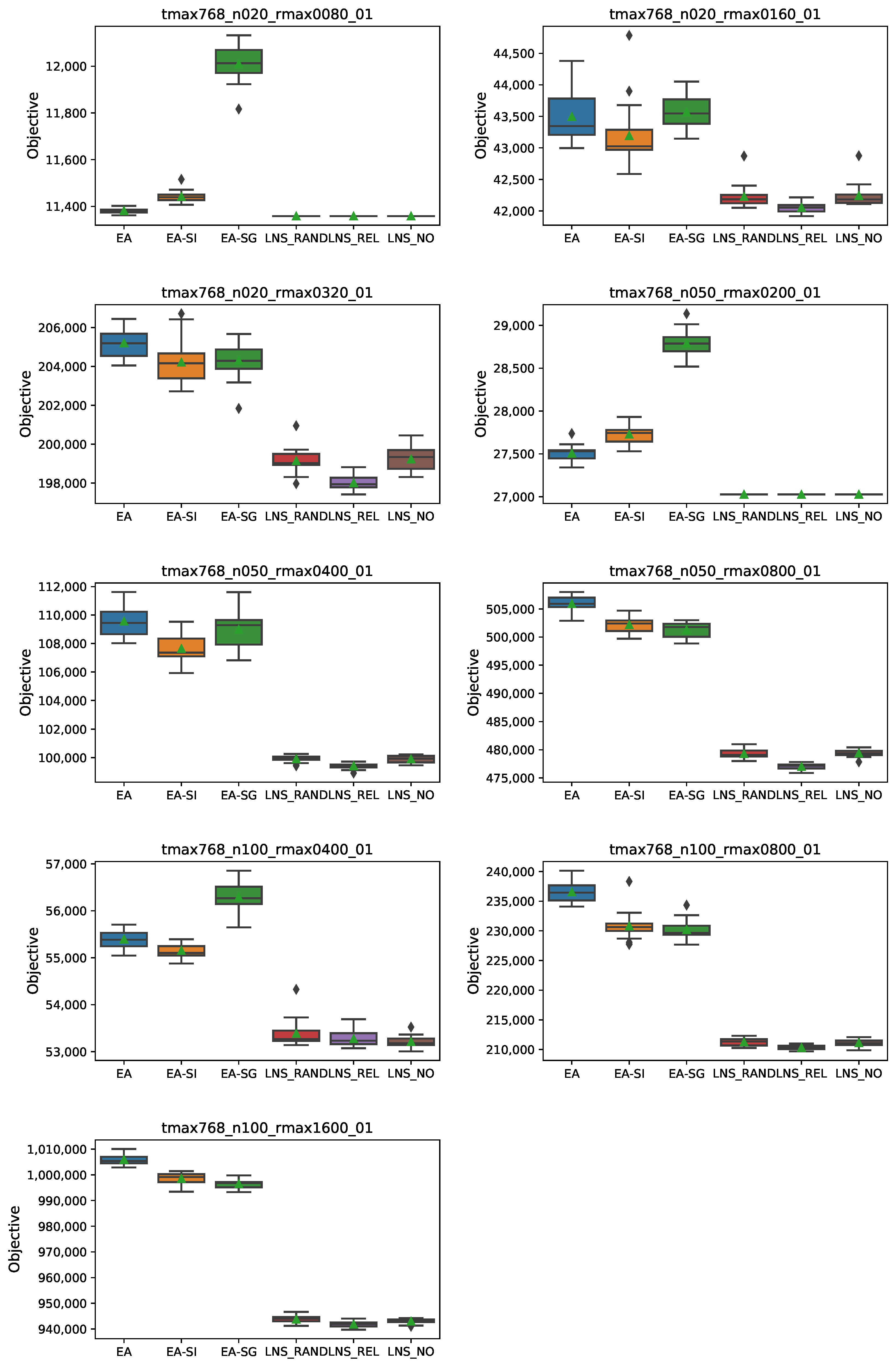
The present work proposed a large neighborhood search approach with a mixed integer linear programming based repair operator for the scheduling of a fleet of shared electric vehicles. Three different destroy operators were evaluated: random destroy, relatedness destroy, and no overlap destroy. The experiments have shown that the proposed approach clearly outperforms not only a standard MILP approach but also a state-of-the-art evolutionary computation-based approach on large instances of the problem yielding between 0.2% and 8.6% better solutions. Of the three investigated destroy operators, relatedness destroy performed best, although it results in the highest runtimes of the insertion operator. On 8 of the 9 considered problem instances, it yielded the best results after a runtime of 60 min. The no overlap destroy operator performed second best and the random destroy operator performed worst. However, also with the random destroy operator, the proposed approach significantly outperformed the evolutionary approach on all considered combinations of time limits and problem instances except for one.

In practice, EV fleet scheduling requires predictions of future PV overproduction, of the energy consumptions corresponding to reservations, and maybe of future electricity prices. A limitation of previous approaches and the approach proposed in the present work is that they do not take uncertainties in these predictions into account. Thus, a potential future work could be to investigate ways to make the approach robust regarding such uncertainties. Another direction of future work could be to develop more efficient destroy operators. The experiments have shown that the choice of the destroy operator has a notable impact on the performance. In recent work, it has been demonstrated that it is possible to learn efficient destroy operators with the help of a data-driven approach [28]. Another question, which could be investigated in the future, is how the EV fleet scheduling performs in a scenario that is more realistic than the synthetic benchmark instances used in the present work.

References

1. Mądziel, M.; Campisi, T. Energy Consumption of Electric Vehicles: Analysis of Selected Parameters Based on Created Database. Energies 2023, 16, 1437. [Google Scholar] [CrossRef]
2. Schmidt, M.; Staudt, P.; Weinhardt, C. Decision support and strategies for the electrification of commercial fleets. Transp. Res. Part D Transp. Environ. 2021, 97, 102894. [Google Scholar] [CrossRef]
3. Vuichard, P. Electrifying the company car: Identifying hard and soft barriers among fleet managers in Switzerland. Energy Res. Soc. Sci. 2021, 77, 102098. [Google Scholar] [CrossRef]
4. Wang, Q.; Liu, X.; Du, J.; Kong, F. Smart Charging for Electric Vehicles: A Survey From the Algorithmic Perspective. IEEE Commun. Surv. Tutorials 2016, 18, 1500–1517. [Google Scholar] [CrossRef] [Green Version]
5. Stadie, M.; Rodemann, T.; Burger, A.; Jomrich, F.; Limmer, S.; Rebhan, S.; Saeki, H. V2B vehicle to building charging manager. In Proceedings of the EVTeC: 5th International Electric Vehicle Technology Conference, Online, 24–26 May 2021. [Google Scholar]
6. Jin, C.; Tang, J.; Ghosh, P. Optimizing Electric Vehicle Charging With Energy Storage in the Electricity Market. IEEE Trans. Smart Grid 2013, 4, 311–320. [Google Scholar] [CrossRef]
7. Igualada, L.; Corchero, C.; Cruz-Zambrano, M.; Heredia, F.J. Optimal Energy Management for a Residential Microgrid Including a Vehicle-to-Grid System. IEEE Trans. Smart Grid 2014, 5, 2163–2172. [Google Scholar] [CrossRef] [Green Version]
8. Franco, J.F.; Rider, M.J.; Romero, R. A Mixed-Integer Linear Programming Model for the Electric Vehicle Charging Coordination Problem in Unbalanced Electrical Distribution Systems. IEEE Trans. Smart Grid 2015, 6, 2200–2210. [Google Scholar] [CrossRef]
9. Naharudinsyah, I.; Limmer, S. Optimal Charging of Electric Vehicles with Trading on the Intraday Electricity Market. Energies 2018, 11, 1416. [Google Scholar] [CrossRef] [Green Version]
10. Schaden, B.; Jatschka, T.; Limmer, S.; Raidl, G.R. Smart Charging of Electric Vehicles Considering SOC-Dependent Maximum Charging Powers. Energies 2021, 14, 7755. [Google Scholar] [CrossRef]
11. Qin, H.; Su, X.; Ren, T.; Luo, Z. A review on the electric vehicle routing problems: Variants and algorithms. Front. Eng. Manag. 2021, 8, 370–389. [Google Scholar] [CrossRef]
12. Bongiovanni, C.; Kaspi, M.; Geroliminis, N. The electric autonomous dial-a-ride problem. Transp. Res. Part B Methodol. 2019, 122, 436–456. [Google Scholar] [CrossRef]
13. Desaulniers, G.; Errico, F.; Irnich, S.; Schneider, M. Exact Algorithms for Electric Vehicle-Routing Problems with Time Windows. Oper. Res. 2016, 64, 1388–1405. [Google Scholar] [CrossRef] [Green Version]
14. Koç, Ç.; Karaoglan, I. The green vehicle routing problem: A heuristic based exact solution approach. Appl. Soft Comput. 2016, 39, 154–164. [Google Scholar] [CrossRef]
15. Schneider, M.; Stenger, A.; Goeke, D. The Electric Vehicle-Routing Problem with Time Windows and Recharging Stations. Transp. Sci. 2014, 48, 500–520. [Google Scholar] [CrossRef] [Green Version]
16. Keskin, M.; Çatay, B. A matheuristic method for the electric vehicle routing problem with time windows and fast chargers. Comput. Oper. Res. 2018, 100, 172–188. [Google Scholar] [CrossRef]
17. Su, Y.; Dupin, N.; Puchinger, J. A deterministic annealing local search for the electric autonomous dial-a-ride problem. Eur. J. Oper. Res. 2023, 309, 1091–1111. [Google Scholar] [CrossRef]
18. Varga, J.; Raidl, G.R.; Limmer, S. Computational Methods for Scheduling the Charging and Assignment of an On-Site Shared Electric Vehicle Fleet. IEEE Access 2022, 10, 105786–105806. [Google Scholar] [CrossRef]
19. Benders, J.F. Partitioning Procedures for Solving Mixed-Variables Programming Problems. Numer. Math. 1962, 4, 238–252. [Google Scholar] [CrossRef]
20. Limmer, S.; Varga, J.; Raidl, G.R. An Evolutionary Approach for Scheduling a Fleet of Shared Electric Vehicles. In Applications of Evolutionary Computation; Springer: Cham, Switzerland, 2023; pp. 3–18. [Google Scholar] [CrossRef]
21. Betz, J.; Werner, D.; Lienkamp, M. Fleet Disposition Modeling to Maximize Utilization of Battery Electric Vehicles in Companies with On-Site Energy Generation. Transp. Res. Procedia 2016, 19, 241–257. [Google Scholar] [CrossRef]
22. Sassi, O.; Oulamara, A. Electric vehicle scheduling and optimal charging problem: Complexity, exact and heuristic approaches. Int. J. Prod. Res. 2017, 55, 519–535. [Google Scholar] [CrossRef]
23. Pisinger, D.; Ropke, S. Large neighborhood search. In Handbook of Metaheuristics; International Series in Operations Research & Management Science 272; Springer: Berlin/Heidelberg, Germany, 2019; pp. 99–127. [Google Scholar]
24. Shaw, P. A New Local Search Algorithm Providing High Quality Solutions to Vehicle Routing Problems; Technical Report; APES Group, Department of Computer Science, University of Strathclyde: Glasgow, UK, 1997. [Google Scholar]
25. Rifai, A.P.; Nguyen, H.T.; Dawal, S.Z.M. Multi-objective adaptive large neighborhood search for distributed reentrant permutation flow shop scheduling. Appl. Soft Comput. 2016, 40, 42–57. [Google Scholar] [CrossRef]
26. Jatschka, T.; Rodemann, T.; Raidl, G.R. A Large Neighborhood Search for a Cooperative Optimization Approach to Distribute Service Points in Mobility Applications. In Metaheuristics and Nature Inspired Computing; Springer: Berlin/Heidelberg, Germany, 2022; pp. 3–17. [Google Scholar]
27. Gurobi Optimization, LLC. Gurobi Optimizer Reference Manual. 2023. Available online: https://www.gurobi.com/wp-content/plugins/hd_documentations/documentation/10.0/refman.pdf (accessed on 5 June 2023).
28. Oberweger, F.F.; Raidl, G.R.; Rönnberg, E.; Huber, M. A Learning Large Neighborhood Search for the Staff Rerostering Problem. In Integration of Constraint Programming, Artificial Intelligence, and Operations Research; Schaus, P., Ed.; Springer International Publishing: Cham, Switzerland, 2022; pp. 300–317. [Google Scholar]
Figure 1. Illustration of the workflow of the large neighborhood search approach.
Energies 16 04576 g001
Figure 2. Boxplot of objective values achieved with different EA and LNS variants after 60 min runtime on different problem instances.
Energies 16 04576 g002