Abstract
Contingency analysis plays an important role in assessing the static security of a network. Its purpose is to check whether a system can operate safely when some elements are out of service. In a real-time application, the computational time required to perform the calculation is paramount for operators to take immediate actions to prevent cascading outages. Therefore, the numerical performance of the contingency analysis is the main focus of this current research. In power flow calculation, when solving the network equations with a sparse matrix solver, most of the time is spent factorizing the Jacobian matrix. In terms of computation time, the symbolic factorization is the costliest operation in the LU (Lower-upper) factorization process. This paper proposes a novel method to perform the calculation with only one symbolic factorization using a full Newton–Raphson-based generic formulation and modular approach (GFMA). The symbolic factorization retained can be used during the iterations of any power flow contingency scenario. A computer study demonstrates that reusing the same symbolic factorization greatly reduces computation time and improves numerical performance. Power system security assessment under N-1 and N-2 contingency conditions is performed for the IEEE standard 54-bus and 108-bus to evaluate the numerical performance of the proposed method. A comparison with the conventional power flow method shows that the time required for the analysis is shortened considerably, with a minimum gain of 228%. The comparative analysis demonstrates that the proposed solution has better numerical performance for large-scale networks.
1. Introduction
Contingency analysis is regarded as an integral part of power system security analysis as it determines the integrity of the power system and verifies the post-contingency equilibrium state in terms of overloads and voltage deviations [1,2]. Its main purpose is to check whether the system can operate safely without any limit violation (i.e., equipment overloading, under- or over-voltage) after the occurrence of a contingency [3].
In N-1 contingency analysis, the main focus is to evaluate the effects of a single equipment outage on power system operating conditions once the single component (such as the loss of a generator, line, and transformer) has been retrieved from the network. Traditional N-1 contingency analysis performs numerous power-flow runs with a total number of N scenarios. After solving the power flow problem for each contingency scenario, the limits are verified for branches and nodes. The system is N-1 secure if, for all scenarios, the following constraints are fulfilled:
The extension of N-1 contingency analysis considers simultaneous component outages (N-k contingencies). N-k security refers to the ability of the system to maintain secure operation after k components have failed in a system with N components [4,5]. For a large-scale network, strict N-k checking requires a large amount of power flow calculation. However, in real-time security assessment, the time window for system operators to analyze the problem and take corrective actions is quite limited. Therefore, the main challenge is to find an efficient method to significantly reduce the resolution time without compromising solution accuracy [6].
In contingency analysis, the power flow method used to perform the contingency analysis has a direct impact on the solution time. The Newton–Raphson power flow-based approach is generally preferred for its superior convergence characteristics and accuracy. The most computationally demanding part of this method is solving the linear equations with LU (Lower-upper) factorization at each iteration. In terms of computation time, the symbolic factorization is the costliest operation in the LU factorization process. This paper focuses on using the Newton–Raphson method to solve contingency analysis. The central question is whether it is possible to avoid the repetitive symbolic factorizations to effectively shorten the analysis time.
We will now highlight the strengths and weaknesses of the most important methods used to reduce the computational time of contingency analysis. This critical literature review will make evident the effectiveness of the proposed solution in simulating the contingency analysis of large-scale networks (Transmission and distribution systems).
The issue of improving computational speed in contingency analysis has been discussed in many works. In [7,8], the compensation theorem is applied to simulate the changes in the passive elements of the network without changing the Jacobian matrix structure. However, this method is well suited to applications involving linear network equations, which is not the case for analysis based fully on Newton’s method.
The main alternative to the compensation method for network matrix modification is to perform partial refactorization [9]. This method consists of updating the LDU (Lower-diagonal-upper) factors to reflect changes in some elements of the Jacobian matrix. The weakness of this method is that the refactorization effort is affected by the position of the modified matrix elements; thus, little or no savings can be obtained if one of the modified elements is near the top of the matrix.
The DC power flow method has been widely used to accelerate the computation of contingency analysis and improve its numerical performance [10]. The DC power flow simplifies the AC power flow to a linear circuit problem. This method is convergent and non-iterative but less accurate than AC power flow solutions.
A reduction in computational time can be achieved by reducing the number of contingency cases to be tried [11,12]. This approach involves ranking contingencies in descending order of severity index. The Contingencies can then be simulated, starting with the most severe and continuing until there is no overloading caused by the outage of branches. The main shortcoming of this method is that the contingency ranking by the index may introduce some errors due to the screening effect.
In [13], the graph theory was used to demonstrate that the base case symbolic factorization can be reused to solve contingency cases. The key assumption of this method is that there is no branch to be put in service during a contingency. This limitation prevents practical use in distribution systems where the introduction of new lines to reroute flows occurs in the most interesting contingencies.
Recent research in the area includes optimization-based methods [14,15,16,17,18,19,20]. These methods do not enumerate every contingency but attempt to find the most severe contingency to reduce the computational burden.
Table 1 demonstrates a summary of the reviewed classical methods for managing contingency analysis, with the major strengths and weaknesses of each one.

Table 1.
Summary of the classical methods of contingency analysis.
Additionally, the aforementioned methods have only addressed cases where the change in the sparsity pattern of the Jacobian matrix is caused by the change in network topology. However, in an automatic adjusting solution [21,22] a new symbolic factorization is not only required for a change involving network topology but also during Newton’s iterative process (due to control adjustment); hence, the symbolic factorization of the base case Jacobian matrix cannot be systematically reused in contingency cases.
In this paper, an original modeling technique has been proposed to avoid the occurrence of change in the sparsity pattern within the same power flow run (due to control adjustments) and after evaluating a new contingency scenario (due to a change in network topology). The proposed solution will overcome the limitations identified in classical methods (Table 1) and allow for the systematic and fast solving of contingency analysis. More specifically, we propose to perform the contingency analysis using only one symbolic factorization. The proposed approach is completely generic and can easily accommodate the simultaneous outages of k-branches in the network (i.e., N-k contingency analysis) with the possibility to include any remedial actions that consist of putting in new service elements.
This paper uses the power flow solver based on GFMA formulation to solve the power flow problem [23]. The algorithm of GFMA is based on the rigorous full Newton–Raphson approach and relies on the automatic adjustment technique, which provides an accurate and fast power flow solution. The high flexibility of this formulation offers the possibility of re-using the base case symbolic factorization of the Jacobian matrix to recompute the power flow of any other scenario. The basic idea behind the proposed approach is to imbue the GFMA power-flow algorithm with the concept of the dynamic parameters to preserve the same sparsity pattern of the Jacobian matrix. The dynamic parameters concept is the main contribution of this research paper.
This paper starts with a brief presentation of the GFMA method for solving power flow problems. The second part presents the modeling concept of dynamic parameters. In the third part, the dynamic parameters are introduced into the component models to perform a unique symbolic factorization in the contingency analysis. The last part presents illustrative simulation examples to evaluate saved time for relatively large transmission networks.
2. GFMA Formulation
The formulation of GFMA is recalled here to establish the basis for the following algorithms. GFMA provides a generic power flow formulation capable of handling complex component models and arbitrary network topology. In this method, each component of a system is modeled autonomously as a subsystem using a non-causal mathematical representation. The implicit representation of the system and the modular approach avoid many theoretical modeling complications, as the variables and load flow constraints can be arbitrarily defined. The GFMA formulation is generic, extensible, and can handle arbitrary component models without any known limitation.
Each component is described using the model representation in the form of Equation (1). For the convenience of the reader, matrices and vectors are indicated in bold type characters.
where:
- uk are the model input variables.
- yk are the model output variables.
- xk are the model internal variables.
- λk are the model variables.
Each model introduces inputs, outputs, and internal state variables. These variables are expressed in real units and can be arbitrarily defined. The voltages are defined as inputs to establish the electrical connection with the connected bus and the currents as outputs to formulate Kirchhoff’s Current Law. The inputs and outputs represent the interface between the model and the system. The readers can refer to [23] for more details.
The component models are aligned along the diagonal to form the equipment Jacobian matrix. This block diagonal matrix is augmented with the linking equations to establish the connection between components. These extra-equations are external to the components model and have a linear form as follows:
where is the output variable of the model; is the input variable of the model; and are the coefficients associated with and , respectively.
Herein, the system is initialized using the single-iteration FP solution [24]. The estimation of the initial guess of the state vector is obtained by converting (1) to the linearized version and solving the resulting linear system of equations in the form of
A comprehensive example is shown in Figure 1 to explore the structure of the Jacobian matrix. As can be seen from Figure 2, the upper and lower block of the Jacobian matrix represent the network equipment and linking equations, respectively. The obtained Jacobian matrix is sparse and unsymmetrical. It is important to notice that the system buses do not contribute to the Jacobian matrix of the system with additional nonzero elements (Figure 2).
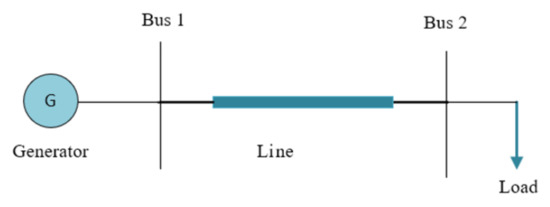
Figure 1.
Test system example.
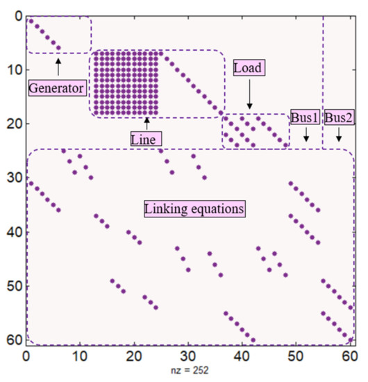
Figure 2.
Matrix structure.
3. Dynamic Parameters Approach
A sparse matrix solver provides efficient numerical solutions to solve linear equations. The KLU solver is suitable for solving unsymmetrical and sparse linear systems [25] and is considered one of the most efficient packages designed for electrical circuits. Roughly speaking, the KLU solver performs two steps in sequence:
- 1.
- Symbolic factorization: performs optimal permutations and pre-ordering to reduce the fill-ins (number of non-zero elements).
- 2.
- Numerical factorization: Computes the factorization sub-matrices L and U.
The change in the Jacobian matrix structure is due to the presence of conditional statements (“if-else”) in the code corresponding to different operating conditions. These conditions are evaluated, and the appropriate constraint equation is executed (see Equation (4)).
The equation can be formulated as one compact mismatch equation.
where:
- fi and λi are the non-linear constraint equation and the dynamic parameter for the ith condition, respectively.
- f0 and λ0 are the linear constraint equation and the dynamic parameter used for the ini-tialization. It is worth noting that the term λ0f0 can be dropped from Equation (5) if the model is linear.
The dynamic parameters approach consists of updating the parameters from iteration to iteration to enforce the appropriate mismatch equation. Specifically, when a new condition is flagged, the parameter associated with the enforced constraint equation is set to one, while the other parameters are all set to zero. This modeling technique prevents a change in the sparsity pattern of the Jacobian matrix since the same mathematical expression holds for all operating conditions.
Equations (4) and (5) are mathematically equivalent but numerically different. The main advantage of formulation (5) resides in its high computational performance since the repetitive symbolic factorizations are systematically avoided.
The dynamic parameters approach has been successfully applied to the power flow problem and will be extended here for contingency analysis. It will be demonstrated in the next section that the use of this modeling technique finds useful applications in network problems involving a change in network topology.
4. Outage Modeling
In this section, the dynamic parameters approach presented in [23] is extended to avoid the symbolic factorizations related to the change in network topology. Herein, the constraint equation enforcing the outage of the equipment () and its associated parameter () are incorporated in the original formulation as follows:
The first term of Equation (6) prevents change in the nonzero pattern of the Jacobian matrix caused by the change in the network topology. To simulate a new contingency scenario, the parameter associated with the localized equipment outage must be set to one. For the base case scenario, the same parameter is set to zero for all elements in the network.
A flowchart depicting the updates in the dynamic parameters in the contingency algorithm is shown in Figure 3.
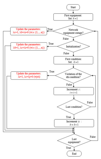
Figure 3.
Updates in the dynamic parameters in the contingency case power flow solution.
From a computational point of view, the constraint equation is considered a judicious choice if the following conditions are fulfilled:
- Condition 1: Ideally, the constraint equation fc should not introduce additional non-zero elements in the Jacobian matrix other than those initially generated from fi.
- Condition 2: A linear constraint equation is preferred, as the Newton–Raphson converges more robustly due to its more linear formulation.
In the following sections, the equations for each model are developed using a compact mismatch equation according to the dynamic parameter approach. For the sake of clarity, the model equations are expressed in complex form, and the partial derivatives are not detailed here, as they can be obtained using the symbolical computation [26].
4.1. Line Outage
The outage of the line is represented by a linear constraint equation forcing the entering currents to zero. For the sake of clarity, the line model of Figure 4 is presented as an example.
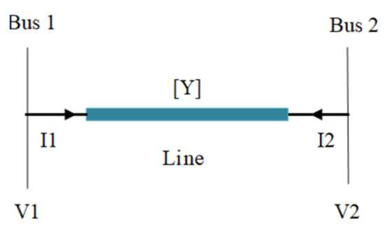
Figure 4.
Line model.
The vector mismatch equation of the line formulated with the dynamic parameters is given by
It should be noted that the linear constraint equation used for the initialization is not required here since the line model is inherently linear.
4.2. Generator Outage
The synchronous generator (SG) is modeled as variable susceptance and conductance ( and ) [23]. The latter two ( and ) are defined in the model as internal state variables which are solved to satisfy the power flow constraints of the machine. This model is numerically more efficient and converges faster than the conventionnel internal voltage behind reactance [27,28].
The SG state variables added to the system’s variables are as follows:
This model introduces eight unknown variables (six for output currents and two for internal variables) required for the solvability of the same number of equations.
For a machine with PV constraint, the mismatch equation written with dynamic parameters is given by
where the active and reactive power is expressed as a function of the state variables
The sign indicates the complex-conjugate operator.
This mismatch equation can capture all possible operating conditions of the machine, including the initialization and equipment outage.
In the initialization stage, the parameter is set to one while all other parameters are set to zero, and the non-linear constraint equations of the generator are reverted to the linearized version. The linear constraint equation is specifically introduced in the mismatch equation to estimate the initial value of the susceptance and conductance. For a machine with PV constraint, and are estimated, assuming a nominal power factor of the machine and the desired active power.
The parameters ,, are dynamically updated during the iterative power flow process to flag all operating conditions of the generator. This allows the machine to switch from PV to PQ when its reactive power limit is violated.
The outage of the generator is represented by an equation forcing the susceptance and conductance to zero. This constraint equation () is linear and does not introduce any additional nonzero elements in the mismatch equation other than those generated from ,,, and . The generator is considered effectively out of service if the parameter is set to one.
Six equations are also introduced from the equation relating the terminal voltages and currents.
where is the Fortescue’s transformation matrix; and are the vector of generator voltages and current in phase domain, respectively.
With the introduction of the dynamic parameters, the constraint Equation (13) becomes
4.3. Transformer Outage
In this section, the transformer outage model is implemented in a three-phase power-flow solution method based on the GFMA formulation. Therein, an ideal transformer connected between nodes and is modeled by describing the voltage and current equations relating the primary and secondary windings. The node is inserted to include the three-phase impedance transformer. This solution is generic and can be used to handle arbitrary transformer connections. The transformer model depicted in Figure 5 is used to derive the constraint equations in the phase domain for an arbitrary three-phase transformer connection.
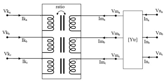
Figure 5.
Three-phase transformer.
The constraint equations for the transformer are given by
where is the three-phase transformer admittance matrix; is the turn ratio of the master transformer; is the dependency that is expressed as a function of turn ratio; and the sign indicates the transpose matrix operator.
The transformer outage is simulated by forcing the output currents at both sides of the transformer to zero. This is achieved by setting the parameter to one.
4.4. Switching Device Outage
For an ideal switch connected between nodes and , the model equation of the switch device depicted in Figure 6 is given by
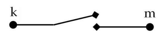
Figure 6.
Switch device.
In this equation, the switch is considered in-service if is set to zero (i.e., closed position). The same equation can be used to simulate the outage of the ideal switch by setting to one (i.e., opened position).
4.5. Load Shedding
An optimal load-shedding scheme is necessary under contingency conditions to prevent cascade outages and complete black-out [29]. The load is formulated using the current-mismatch equations [30,31]. The load mismatch equation is given by
where and are the voltages at nodes and , respectively; is the injected load current; and is the estimated load admittance used for the initialization.
5. General Aspects of the Algorithm
With the introduction of the dynamic parameters in the formulation of mismatch equations, the sparsity pattern of the Jacobian matrix corresponding to the base case scenario becomes identical to that of any contingency case. The unique symbolic factorization retained in all scenarios of contingency analysis corresponds to that performed for the system initialization of the base case scenario.
In the base case scenario, all the network equipment is initially in service. However, any equipment that was initially out of service but expected to be connected as part of remedial action must be included in the base case scenario and modeled as an out-of-service element. From a modeling point of view, adding and removing an element from the system are treated similarly.
Simultaneous outages (N-2) are treated as single outages (N-1). Both can reuse the symbolic factorization of the base case scenario.
The main drawback of the proposed approach is that the nonzero elements and the size of the Jacobian matrix in the contingency cases are slightly overestimated. To illustrate this point, let us consider an outage of a transmission line that is modeled using dynamic parameters. The Jacobian elements are obtained by replacing the dynamic parameter in Equation (7) with one and then deriving the partial derivatives with respect to the state variables. Expressed in real form, the Jacobian elements of the positive sequence model of the line are given by
As can be seen from Equation (18), eight nonzero elements contribute to removing a branch element from the system. These elements will exist only if the symbolic factorization of the base case scenario is reused for the contingency scenario. This is evident from the fact that all elements in the base case are initially considered in service. It is worth noting that the KLU solver does not drop numerically zero entries from its sparse matrix; therefore, all the entries that are present in the data structure of the Jacobian matrix are not dropped, even though they are numerically zero.
The contingency analysis is performed with the algorithm depicted in Figure 7.
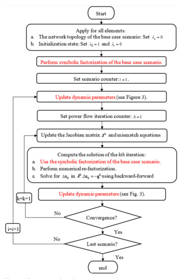
Figure 7.
Contingency algorithm.
6. Validation
The proposed solution has been tested for the IEEE 57-bus and the IEEE 118-bus test systems. These networks are used to evaluate the numerical performance of the proposed solution. The objective is to compare the computational cost of the proposed solution (GFMA) with the contingency analysis method implemented in CYME power engineering software. This conventional method consists of performing extensive simulations and the strict checking of all possible contingencies using a MANA (Modified-augmented-nodal-analysis)-based power flow solution [32,33]. MANA and GFMA are two different formulations, but both are implemented in a-b-c reference frame and solved using the full-Newton algorithm and KLU solver.
Herein, the simulations are performed for the N-1 and N-2 security criteria. The N-1 criterion considers a unique contingency that is cleared by the primary protection, in this case, the faulted element is disconnected from the system without any further impact on the system. However, the N-2 criterion considers that the first outage in the system results in a second component failure. It is worth noting that the N-k security criterion leads to possible contingencies ().
To evaluate the resolution time of the contingency analysis, timers were inserted into the code sections, where the symbolic and numerical factorizations are performed. The normalized CPU time with respect to the proposed solution is presented at the end of this section, and a comparison between the numerical efficiency of these two methods serves as a closing statement.
All algorithms have been programmed and executed using the MATLAB Platform, which runs on a dedicated machine (3.4 GHz i7-2600 CPU with 16 GB of RAM). A tolerance of 0.01% on the voltage mismatch is used as the stopping criterion for each power flow run.
6.1. Case-1: IEEE 57-Bus Test System
The IEEE 57-bus system shown in Figure 8 is used to test the numerical performance of the proposed method and to assess the gain in computation time. The network contains 57 buses, 63 lines, 7 generators, 15 two-winding transformers, and 42 loads. The total number of components that can potentially fail in the system is 85 (). Contingency is carried out using the GFMA formulation proposed in this paper and MANA formulation implemented in CYME software.
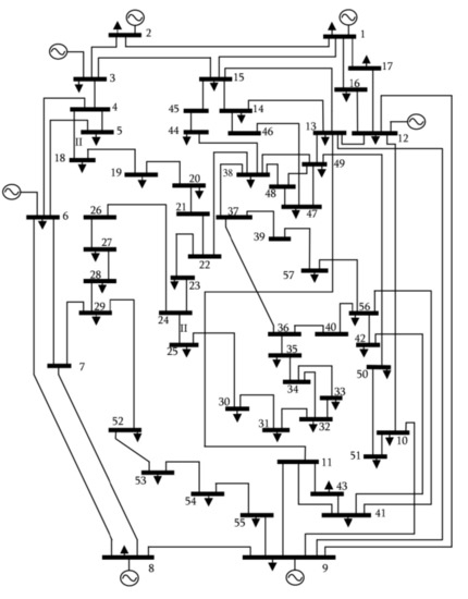
Figure 8.
IEEE 57-bus System.
The strict N-l of the IEEE 57-bus system needs 85 () outage analyses. Table 2 shows that both methods require the same number of numerical factorizations; however, the number of symbolic factorizations required in the MANA is 190, while the proposed solution performs the same calculation with only one symbolic factorization. Moreover, when the nonzero pattern is already known, the depth-first search used in Gilbert/Peierls method can be skipped. This means that numerical factorization becomes computationally less expensive when the sparsity pattern is not changed. Therefore, the cost of the numerical factorization is smaller for GFMA than MANA. In this case, the GFMA is about 2.30 faster than MANA (Table 2).
Table 2.
CPU Timings for the N-1 contingency analysis using MANA and GFMA.
For N-2 contingency analysis, the IEEE 57-bus system needs 3570 scenarios (). As expected, the CPU time is significantly reduced since one symbolic factorization is performed to evaluate this large number of outage scenarios. In this case, the GFMA is about 2.28 faster than MANA (Table 3). Although the performance ratio depends on the system size and the number of controller devices, this case study clearly demonstrates that the time required for the analysis is shortened considerably with the use of the proposed method.
Table 3.
CPU Timings for the N-2 contingency analysis using the MANA and GFMA.
The sparsity pattern of the Jacobian matrix of the base case scenario has a dimension of with 16,242 nonzero elements (see Figure 9). The matrix structure of the base case scenario is identical to any contingency case.
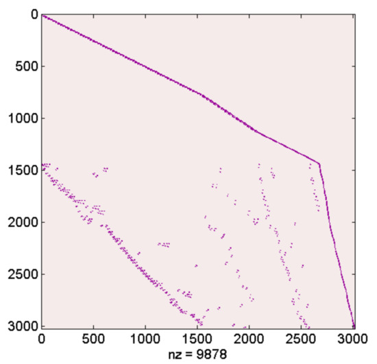
Figure 9.
Sparsity pattern of the Jacobian matrix of the base case scenario (IEEE 57-bus System).
6.2. Case-2: IEEE 108-Bus Test System
This IEEE 108-bus test system was used in various studies for contingency evaluation and voltage security assessment. This system contains 19 generators, 35 synchronous condensers, 177 lines, 9 transformers, and 91 loads (Figure 10). The total number of components is 240 (). The strict N-l and N-2 checking of the IEEE 108-bus system needs 240 and 3570 outage analyses, respectively.
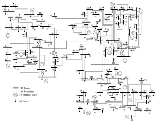
Figure 10.
IEEE 118-bus test system.
The comparative analysis presented in Table 2 and Table 3 leads to the same findings as those observed in the IEEE 54-bus system. Once more, the proposed solution proves to be faster than MANA, with a significant reduction in resolution time.
In addition, the proposed method performs better for larger systems and its efficiency increases as the system increases in size. This can be observed from the results of Table 2 and Table 3, where the detailed CPU time is provided for both networks (IEEE-54 and IEEE-108 systems). This is explained by the fact that the number of symbolic factorizations required to cover all contingencies increases drastically with the size of the network.
7. Conclusions
The proposed modeling technique presented in this paper exploits the flexibility of the GFMA formulation to avoid the repetitive symbolic factorizations required during the iterative power flow process and after the modification of network topology. Herein, the contingency analysis is performed with only one symbolic factorization using a Newton-like method and KLU sparse matrix solver.
The proposed approach is completely generic and can be applied to simulate simultaneous outages of k-branches elements in the network and any remedial actions that consist of putting in service new elements. The proposed solution is generic and can be applied to the strict N-k checking without any known limitation.
The new method has been tested on IEEE 57-bus and IEEE 108-bus test systems, with all the details represented and simulated. The power system security assessment under N-1 and N-2 contingency conditions demonstrates that a significant computational gain has been achieved by applying the concept of dynamic parameters. The results also showed that the method performs better for larger systems and that its efficiency increases as the system increases in size.
Author Contributions
Conceptualization, H.B.; methodology, H.B.; software, H.B.; validation, H.B.; formal analysis, H.B.; investigation, H.B.; resources, H.B.; data curation, H.B.; writing—original draft preparation, H.B.; writing—review and editing, H.B. and A.C.; visualization, H.B.; supervision, A.C. and A.E.O.; project administration, A.C. and A.E.O.; funding acquisition, A.E.O. All authors have read and agreed to the published version of the manuscript.
Funding
Financial support from the University of Quebec at Rimouski under grant AEO-760700.
Data Availability Statement
Not applicable.
Acknowledgments
The financial support from the University of Quebec at Rimouski under grant AEO-760700 is gratefully acknowledged.
Conflicts of Interest
The authors declare no conflict of interest.
References
- Kip, M.; Lei, W.; Prabha, K. Power system security assessment. IEEE Power Energy Mag. 2004, 2, 30–39. [Google Scholar]
- Mohammed, S.; William, T.; Yong, F. Impact of Security on Power Systems Operation. Proc. IEEE 2005, 93, 2013–2025. [Google Scholar]
- Bulat, H.; Franković, D.; Vlahinić, S. Enhanced Contingency Analysis—A Power System Operator Tool. Energies 2021, 14, 923. [Google Scholar] [CrossRef]
- Liana, C.; Xuan, L.; Zuyi, L. Preventive Mitigation Strategy for the Hidden N-k Line Contingencies in Power Systems. IEEE Trans. Reliab. 2018, 67, 1060–1070. [Google Scholar]
- Babalola, A.; Belkacemi, R.; Zarrabian, S. Real-time cascading failures prevention for multiple contingencies in smart grids through a multi-agent system. IEEE Trans. Smart Grid 2018, 9, 373–385. [Google Scholar] [CrossRef]
- Hassan, H.; Mehrdad, T.; Pedram, S. Accurate, simultaneous and Real-Time screening of N-1, N-k, and N-1-1 contingencies. Int. J. Electr. Power Energy Syst. 2022, 136, 107592. [Google Scholar] [CrossRef]
- William, F.T. Compensation Methods for Network Solutions by Optimally Ordered Triangular Factorization. IEEE Trans. Power Appar. Syst. 1972, PAS-91, 123–127. [Google Scholar]
- Ongun, A.; Brian, S.; William, F.T. Sparsity-Oriented Compensation Methods for Modified Network Solutions. IEEE Trans. Power Appar. Syst. 1983, PAS-102, 1050–1060. [Google Scholar]
- Sherman, M.C.; Vladimir, B. Partial Matrix Refactorization. IEEE Trans. Power Syst. 1986, 1, 193–199. [Google Scholar]
- John, K.; Felix, W. Analysis of linearized decoupled power flow approximations for steady-state security assessment. IEEE Trans. Circuits Syst. 1984, 31, 623–636. [Google Scholar]
- Mikolinnas, T.A.; Bruce, W. An Advanced Contingency Selection Algorithm. IEEE Power Eng. Rev. 1981, 2, 25–26. [Google Scholar] [CrossRef]
- Halpin, T.F.; Robert, F.; Fink, R. Analysis of automatic contingency selection algorithms. IEEE Power Eng. Rev. 1984, 5, 29–30. [Google Scholar]
- Elliott, M.C.; Jingjin, W.; Yiting, Z.; Renchang, D.; Guangyi, L. Symbolic Factorization Re-utilization for Contingency Analysis. In Proceedings of the IEEE Power & Energy Society General Meeting (PESGM), Portland, OR, USA, 5–10 August 2018; pp. 1–5. [Google Scholar]
- Pudi, S.; Sanjeeb, M. Power system contingency ranking using Newton Raphson load flow method. In Proceedings of the Annual IEEE India Conference (INDICON), Mumbai, India, 13–15 December 2013; pp. 1–4. [Google Scholar]
- Rocco, C.M.; Ramirez-Marquez, J.E.; Salazar, D.E.; Yajure, C. Assessing the Vulnerability of a Power System Through a Multiple Objective Contingency Screening Approach. IEEE Trans. Reliab. 2011, 60, 394–403. [Google Scholar] [CrossRef]
- Ding, T.; Li, C.; Yan, C.; Li, F.; Bie, Z. Bilevel Optimization Model for Risk Assessment and Contingency Ranking in Transmission System Reliability Evaluation. IEEE Trans. Power Syst. 2017, 32, 3803–3813. [Google Scholar] [CrossRef]
- Street, A.; Oliveira, F.; Arroyo, J.M. Contingency-Constrained Unit Commitment with n–K Security Criterion: A Robust Optimization Approach. IEEE Trans. Power Syst. 2011, 26, 1581–1590. [Google Scholar] [CrossRef]
- Wang, Q.; Watson, J.; Guan, Y. Two-stage robust optimization for N-k contingency-constrained unit commitment. IEEE Trans. Power Syst. 2013, 28, 2366–2375. [Google Scholar] [CrossRef]
- Levitin, G. Optimal Defense Strategy Against Intentional Attacks. IEEE Trans. Reliab. 2007, 56, 148–157. [Google Scholar] [CrossRef]
- Levitin, G.; Hausken, K. Redundancy vs. Protection vs. False Targets for Systems Under Attack. IEEE Trans. Reliab. 2009, 58, 58–68. [Google Scholar] [CrossRef]
- Stott, B. Review of load-flow calculation methods. Proc. IEEE 1974, 62, 916–929. [Google Scholar] [CrossRef]
- Norris, M.P.; Scott, M. Automatic Adjustment of Transformer and Phase-Shifter Taps in the Newton Power Flow. IEEE Trans. Power Appar. Syst. 1971, PAS-90, 103–108. [Google Scholar]
- Hakim, B.; Ahmed, C.; Abderrazak, E. A generic three-phase power flow formulation for flexible modeling and fast solving for large-scale unbalanced networks. Int. J. Electr. Power Energy Syst. 2023, 148. [Google Scholar]
- Wilsun, X.; Hermann, W.D.; José, R.M. Generalized three-phase power flow method for the initialization of EMTP simulations. In Proceedings of the POWERCON ’98. 1998 International Conference on Power System Technology. Proceedings (Cat. No.98EX151), Beijing, China, 18–21 August 1998; Volume 2, pp. 875–879. [Google Scholar]
- Timothy, A.D.; Eknathan, P.N. Algorithm 907: KLU, a direct sparse solver for circuit simulation problems. ACM Trans. Math. Softw. 2010, 37, 3. [Google Scholar]
- Canizares, C.A. Applications of symbolic computation to power system analysis and teaching. In Proceedings of the 2006 PES Power Systems Conference and Exposition, Atlanta, GA, USA, 29 October–1 November 2006; p. 361. [Google Scholar]
- Chen, T.H.; Chen, M.S.; Inoue, T.; Kotas, P.; Chebli, E.A. Three-phase cogenerator and transformer models for distribution system analysis. IEEE Trans. Power Deliv. 1991, 6, 1671–1681. [Google Scholar] [CrossRef]
- Tatianna, B.; Penido, D.R.R.; Araujo, L.R. A new synchronous DG model for unbalanced multiphase power flow studies. IEEE Trans. Power Syst. 2020, 35, 803–813. [Google Scholar]
- Bhuvanagiri, R.; Mohan, K.; Surya, V. Priority Based Optimal Load Shedding in a Power System Network under Contingency Conditions. In Proceedings of the International Conference for Advancement in Technology (ICONAT), Goa, India, 21–22 January 2022; pp. 1–5. [Google Scholar]
- Sereeter, B.; Vuik, K.; Witteveen, C. Newton Power Flow Methods for Unbalanced Three-Phase Distribution Networks. Energies 2017, 10, 1658. [Google Scholar] [CrossRef]
- Garcia, P.; Pereira, J.; Carneiro, S.; Da Costa, V.; Martins, N. Three-phase power flow calculations using the current injection method. IEEE Trans. Power Syst. 2000, 15, 508–514. [Google Scholar] [CrossRef]
- Ilhan, K.; Jean, M.; Ulas, K.; Gurkan, S.; Omar, S. Multiphase Load-Flow Solution for Large-Scale Distribution Systems Using MANA. IEEE Trans. Power Deliv. 2014, 29, 908–915. [Google Scholar]
- Jean, M. Régimes transitoires électromagnétiques: Simulation. In Réseaux Électriques et Applications; TECHNIQUES DE L’INGENIEUR: Saint-Denis, France, 2015. [Google Scholar]
Disclaimer/Publisher’s Note: The statements, opinions and data contained in all publications are solely those of the individual author(s) and contributor(s) and not of MDPI and/or the editor(s). MDPI and/or the editor(s) disclaim responsibility for any injury to people or property resulting from any ideas, methods, instructions or products referred to in the content. |
© 2023 by the authors. Licensee MDPI, Basel, Switzerland. This article is an open access article distributed under the terms and conditions of the Creative Commons Attribution (CC BY) license (https://creativecommons.org/licenses/by/4.0/).