Article

Predicting Biomass Yields of Advanced Switchgrass Cultivars for Bioenergy and Ecosystem Services Using Machine Learning

1
Environmental Science Division, Argonne National Laboratory, 9700 S. Cass Ave., Lemont, IL 60439, USA
2
Department of Crop Science, University of Illinois Urbana-Champaign, 1102 S. Goodwin Ave., Urbana, IL 61801, USA
3
Department of Agronomy, Iowa State University, 1223 Agronomy Hall, Ames, IA 50011, USA
*
Author to whom correspondence should be addressed.
Energies 2023, 16(10), 4168; https://doi.org/10.3390/en16104168
Submission received: 1 April 2023 / Revised: 4 May 2023 / Accepted: 10 May 2023 / Published: 18 May 2023
(This article belongs to the Special Issue Energy – Machine Learning and Artificial Intelligence)

Abstract

:
The production of advanced perennial bioenergy crops within marginal areas of the agricultural landscape is gaining interest due to its potential to sustainably produce feedstocks for biofuels and bioproducts while also improving the sustainability and resilience of commodity crop production. However, predicting the biomass yields of this production system is challenging because marginal areas are often relatively small and spread around agricultural fields and are typically associated with various abiotic conditions that limit crop production. Machine learning (ML) offers a viable solution as a biomass yield prediction tool because it is suited to predicting relationships with complex functional associations. The objectives of this study were to (1) evaluate the accuracy of commonly applied ML algorithms in agricultural applications for predicting the biomass yields of advanced switchgrass cultivars for bioenergy and ecosystem services and (2) determine the most important biomass yield predictors. Datasets on biomass yield, weather, land marginality, soil properties, and agronomic management were generated from three field study sites in two U.S. Midwest states (Illinois and Iowa) over three growing seasons. The ML algorithms evaluated in the study included random forests (RFs), gradient boosting machines (GBMs), artificial neural networks (ANNs), K-neighbors regressor (KNR), AdaBoost regressor (ABR), and partial least squares regression (PLSR). Coefficient of determination (R2) and mean absolute error (MAE) were used to evaluate the predictive accuracy of the tested algorithms. Results showed that the ensemble methods, RF (R2 = 0.86, MAE = 0.62 Mg/ha), GBM (R2 = 0.88, MAE = 0.57 Mg/ha), and GBM (R2 = 0.78, MAE = 0.66 Mg/ha), were the most accurate in predicting biomass yields of the Independence, Liberty, and Shawnee switchgrass cultivars, respectively. This is in agreement with similar studies that apply ML to multi-feature problems where traditional statistical methods are less applicable and datasets used were considered to be relatively small for ANNs. Consistent with previous studies on switchgrass, the most important predictors of biomass yield included average annual temperature, average growing season temperature, sum of the growing season precipitation, field slope, and elevation. This study helps pave the way for applying ML as a management tool for alternative bioenergy landscapes where understanding agronomic and environmental performance of a multifunctional cropping system seasonally and interannually at the sub-field scale is critical.

1. Introduction

Interest in the sustainable co-production of commodity crops and perennial bioenergy crops is increasing due to its promising agricultural and environmental benefits [1]. A major driving factor of this interest is the potential use of marginal lands for perennial bioenergy crop production (areas within agricultural landscapes that have sub-optimal growing conditions for commodity crops and/or high susceptibility to environmental quality degradation [2]). Targeting marginal lands and selecting advanced (high-yielding) perennial bioenergy crop cultivars could aid the production of sustainable biofuels and derivative products (bioplastics, biochemicals, etc.) while enhancing the ecosystem services of the agricultural production systems [2,3,4]. Additionally, this production approach can help address indirect land use change, a major concern for large-scale lignocellulosic biomass production [5,6].
Commodity crops (corn, soybeans, wheat, etc.) grown on marginally productive lands can have negative environmental consequences, such as nutrient leaching and soil erosion [3]. Perennial bioenergy crops systematically located either along the edges of fields or on marginal lands can capture excess nutrients from adjacent commodity crops and minimize impacts on the downstream surface water quality [3,4,7]. Water quality improvements and other environmental benefits resulting from this type of integrated production system can also be monetized and help lower the overall production costs of biofuels and derivative products [8]. The use of high-yielding perennial energy crop cultivars, which are relatively well-suited to marginal conditions, could boost sustainable biomass production with reduced competition with commodity crop production. However, as a new cropping system, it has logistical and technical challenges. For instance, predicting the yields of advanced perennial bioenergy crop cultivars under this proposed production system is a challenge due to the variability in size and distribution of marginal lands within agricultural landscapes [2]. Overcoming barriers to their adoption requires, among others, the development of new management practices and tools for accurate quantification of energy crop productivity and associated economic and environmental benefits [9].
To maximize economic opportunities and achieve the desired environmental benefits, the uncertainty and risks of integrating bioenergy crops into commodity cropping systems must be assessed and mitigated [8,10]. This requires an understanding of the agronomic, economic, and environmental performance of the integrated system across multiple production years and at various production scales (e.g., field, watershed, and regional). This effort also requires accurate computer models that can predict the end-of-the-growing-season biomass yield and extrapolate findings from sparse field studies to targeted production regions with similar growing conditions [10,11,12].
Predictive models can inform techno-economic and life-cycle analyses that are designed to evaluate the economic viability and opportunities and environmental performance of a feedstock supply chain needed for the bioeconomy. Land marginality or landscape position, combined with growing conditions and agronomic practices, affect harvestable yields across crop types [13]. Variability in biomass yield, in addition to biomass quality, are major challenges to feedstock preprocessing and conversion operation efficiencies [14]. Predicting biomass yield for a specific bioenergy crop cultivar as a function of land marginality/landscape position, environmental conditions, and crop management is a complex problem. Creating a process-based model that integrates all of these complex and interdependent biophysical, geochemical, and crop management factors to predict biomass yield across multiple scales (sub-field to field to watershed to regional scale) is challenging, as it requires a large amount of data processing in addition to a mechanistic understanding of sparsely observed ecosystem processes [13,15]. Using statistics-based models may not be an option because, among other factors, the mathematical relationships describing the physiological and biochemical compositional characteristics of newly developed cultivars as a function of land marginality, growing conditions, and crop management are still developing.
Machine learning (ML), the sub-field of computer science concerned with techniques that enable computers to learn domain insights without explicit programming [16], provides a viable alternative to process-based and statistics-based models for generating valuable, timely information needed for techno-economic and life-cycle analyses and other efforts toward realizing a sustainable bioeconomy. ML is well-suited for predicting biomass yield because the prediction of biomass involves relationships between the response and explanatory variables with multiple or complex functional associations (linear, nonlinear, mixed, etc.). While ML has been used for predicting the yields of corn, soybeans, wheat, and other agricultural crops [13,17,18,19,20,21], applying the approach to predicting the biomass yields of advanced perennial bioenergy crops, especially advanced switchgrass cultivars that are grown under agriculturally marginal lands of the U.S. Midwest, has not been widely explored [15].
Wullschleger et al. [22] used the generalized additive model (GAM) [23] to determine the important predictors of bioenergy switchgrass yield. A total of 1190 observations of biomass yield from multiple cultivars across 39 sites in 17 U.S. states were generated through a survey of 18 publications. They found climate, agronomic practices (e.g., N fertilization rates), and ecotype (lowland vs. upland) to be the important predictors of switchgrass biomass yield. Tulbure et al. [24] utilized the same data sources as [22] and further assessed the important drivers of the variability in bioenergy switchgrass yield. Their spatio-temporal analysis results showed that climate variability is the primary predictor of yield variability. A more recent study [25] was conducted using 900 biomass yield observations compiled from 41 field trials in the U.S. to assess variability in the yields of four switchgrass cultivars in the context of location of origin, adaptation to local growing conditions, and future climate scenarios. Using a random forest model, Zhang et al. [25] found that climate and management variables are the more important predictors of yield compared with soil parameters. However, these studies were using only predecessor cultivars intended for large-scale monocultural production instead of utilizing advanced switchgrass cultivars targeting marginal agricultural production areas. More importantly, no single cultivar was grown across the multiple field trial locations during the same cropping year where the yield data were generated. Additionally, these studies focused only on one ML algorithm instead of evaluating multiple ML algorithms that have been widely used for agricultural applications.
Future perennial bioenergy cropping systems are likely to be dominated by advanced cultivars due to their relatively higher biomass yield compared with their predecessors. Development of a data-driven tool with predictive capabilities of the biomass yield of advanced switchgrass cultivars for bioenergy, given such factors as land marginality, crop growing conditions, and crop management practices, is needed to help overcome logistical and technical barriers to adoption. An accurate modeling tool will increase our capabilities in mitigating risks and uncertainty assessment in (1) identifying localities or regions where marginal lands are suited for specific bioenergy crop species or cultivars that could produce biofuels of the desired range of qualities economically and (2) locating and designing the preprocessing and conversion systems. This predictive tool will also enable us to gain an improved understanding of performance over gradients of geographic range and soil conditions, which can enable research prioritization and facilitate adoption by stakeholders. The objectives of this study were to (1) compare ML algorithms and identify the top performers in predicting the biomass yields of advanced cultivars at the end-of-the-growing-season harvest and (2) identify the most important predictors or explanatory variables of advanced switchgrass cultivar biomass yields grown in marginal croplands.

2. Materials and Methods

2.1. ML Modeling Workflow

The ML modeling approach in this study comprised two main phases, namely learning and prediction (Figure 1). The learning phase included the identification of the relevant data and their sources (Step 1), data fusion (Step 2), and algorithm training and testing (within Step 3, model exploration/learning). Testing used the most accurate algorithm and its associated optimized parameters from the learning phase to predict biomass yield in the prediction phase. Detailed data descriptions and their respective sources (Step 1) can be found in Section 2.3. Data were preprocessed and evaluated for quality (Step 2). Preprocessed data were then used to generate gridded (10 m raster) datasets. Shapefiles for each plot (Figure 2) were used to determine zonal statistics. Variables were summarized and used to evaluate each algorithm (Section 2.4).
Python 3.9 [26] was used to employ computational science software, including pandas [27], NumPy [28], and scikit-learn [29].

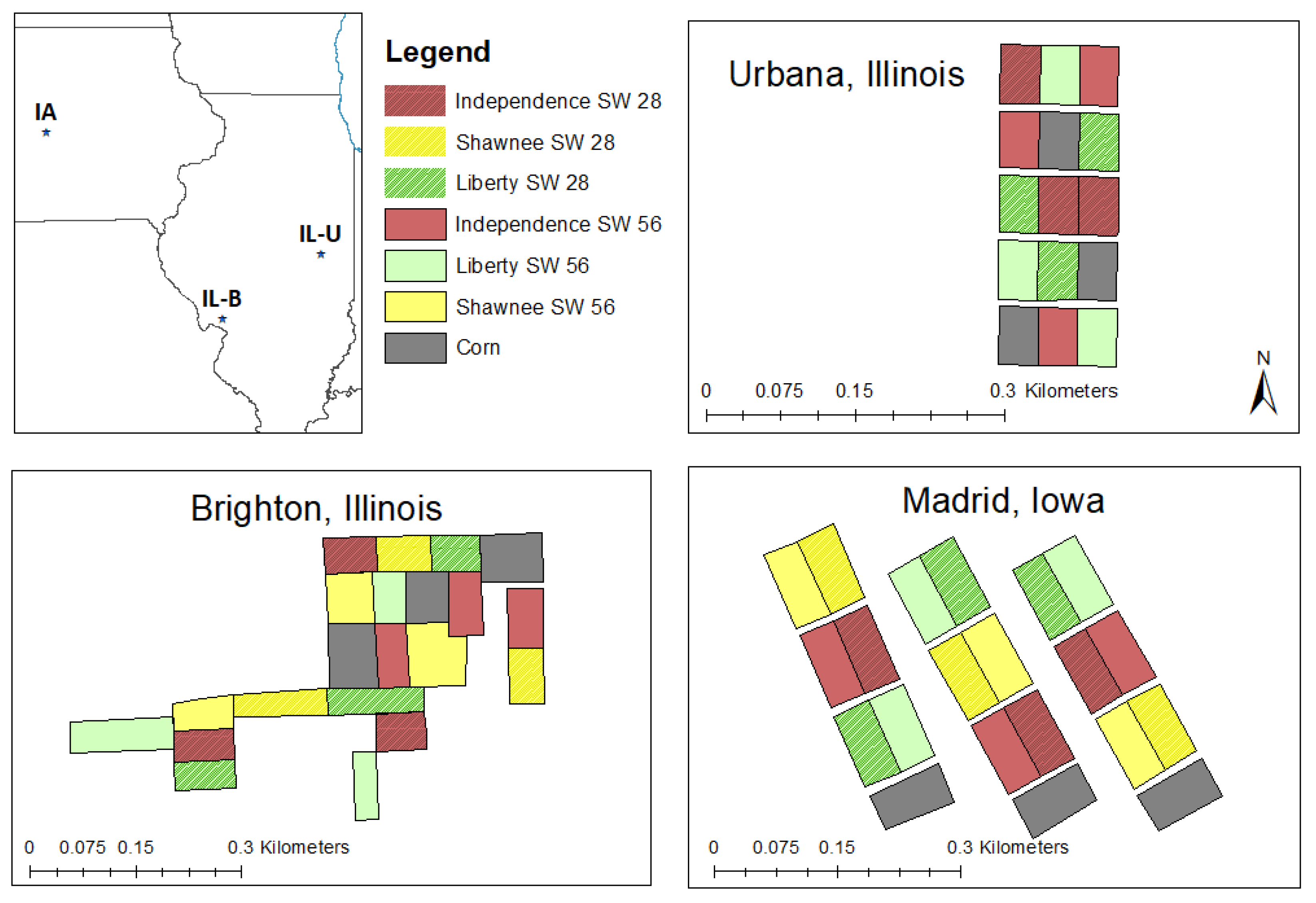
2.2. Description of Field Study Sites and Experimental Setup

Large-scale field trials evaluating the biomass production of high-yielding, warm-season perennial bioenergy grasses were conducted across several U.S. Midwest states, as described in Hamada et al. [30]. For this analysis, we focused on three of the field sites (Brighton, Illinois; Urbana, Illinois; and Madrid, Iowa) due to similarities in the switchgrass cultivars evaluated (Figure 2). Two advanced, high-yielding cultivars, Independence and Liberty, were included along with a predecessor variety called Shawnee (Table 1). Field sites were on marginal lands not suitable for row crop production due to their historically low yields of crops, including corn, soybeans, or wheat, in their region [30]. The experimental designs for each field site are shown in Figure 2, including nitrogen (N) application rates, which began to be applied starting in the second production year. In Iowa and Brighton, Illinois, switchgrass plots were established in the spring of 2019, whereas the Urbana, Illinois, site was established in the following spring of 2020. Additional descriptions of these sites can be found in Hamada et al. [30].

2.3. Data and Sources

The data used in this study included climatic factors, land marginality classification, soil properties, topographic characteristics, crop management, and crop attributes, which were generated from each of the three study sites described in Section 2.2. Some of the data were measured at the study sites (manually and through dedicated monitoring systems); others were derived from online databases (e.g., U.S. Soil Survey Geographic Database (SSURGO) of the U.S. Department of Agriculture—Natural Resources Conservation Service (USDA-NRCS), Global Historical Climatology Network of the National Oceanic and Atmospheric Administration (NOAA), and National Elevation Dataset of the U.S. Geological Survey); and the remainder were generated using remote sensing. Details of all the tested model variables, including their descriptions, types, and units, are presented in Appendix A (Table A1).

2.3.1. Climatic Factors

The choice of climatic factors used in this study was based on the findings of Tulbure et al. [24], who conducted a modeling study on the genetic and climatic controls of lowland and upland switchgrass ecotypes. They found that total precipitation for April–May and June–September and the average temperature of the growing season are the most critical factors for predicting yields of lowland and upland switchgrass cultivars. In this study, we added the annual average temperature to represent the combined effect of the differences in winter, spring, and summer temperatures [31].
Climatic data were generated from field-installed weather stations (two at each study site—one in a switchgrass plot and another in a corn plot), from nearby Mesonet, and from the NOAA’s Global Historical Climatology Network stations (Table A2). Point-observed values from these stations, along with their respective coordinates and elevation values, were used to generate gridded datasets of total precipitation for April–May, total precipitation for June–September, average temperature of the growing season, and annual average temperature using the inverse distance weighting (IDW) method [32]. IDW is one of the most widely used deterministic spatial methods for spatial interpolation of precipitation data [33] The IDW method was performed using ArcGIS Desktop 10.4.1 (ESRI, Redlands, CA, USA).

2.3.2. Land Marginality

Land marginality classification in this study was based on metrics proposed by Ssegane and Negri [2]. In this context, the marginality of an area within the field is identified on the basis of commodity crop yield and environmental quality indicators. Land marginality factors included in this study were the national commodity crop productivity index, soil drainage class, ponding frequency, and flooding frequency. An area is considered marginal if it has an inherently low to very low crop productivity index, is frequently ponded and flooded, and is poorly to very poorly drained.
Feature layers for each of the marginality factors were generated using the USDA-NRCS’s Soil Data Viewer, which integrates the soil shapefiles and their corresponding tabular data. Binary raster layers were then generated from these feature layers using the ArcGIS Desktop for each land marginality factor, where marginal and nonmarginal pixels were assigned values of 1 and 0, respectively.

2.3.3. Soil Properties

Soil properties used in this study were generated from the SSURGO database. The soil depth of interest was the top 30 cm of the soil horizon, where most of the switchgrass root biomass resides [34,35] and soil macro and microorganisms are most active [36]. Soil properties used as explanatory variables included bulk density, soil organic matter content, soil texture (percentages of sand, silt, and clay), available soil water capacity, cation exchange capacity, and soil pH. Soil properties—particularly soil organic matter content—explained approximately 30% of the yield variability of corn from multiple fields in central Illinois and eastern Indiana in the United States [37]. Jiang and Thelen [38] found very fine sand content, clay content, and pH as important soil properties in explaining corn yield variability in the corn fields under corn–soybean rotation in Michigan (USA). Tulbure et al. [24], who studied environmental and genetic controls of switchgrass yields across 15 states in the U.S., found soil texture to be an important explanatory variable, particularly sand and clay content.

2.3.4. Topography

Elevation, slope, and curvature were the three topographic characteristics considered to be important predictors of crop yield. Approximately 20% of variability in the corn yields from multiple fields in central Illinois and eastern Indiana in the United States was explained by the combined effect of topographic characteristics, with elevation being the most influential [37]. Slope and elevation were also found to be important factors for explaining corn yield variability in the fields of Michigan [38]. A 10 m digital elevation model (DEM) from the USDA-NRCS Geospatial Data Gateway [39] was used in this study. Both slope and curvature were generated from the DEM layer using ArcGIS Desktop 10.4.1.

2.3.5. Crop Management and Biomass Yield

The crop management practice that was included as an explanatory variable is the nitrogen (N) fertilization rate, which is an important predictor of switchgrass yield [26]. In this study, switchgrass was fertilized with N at 28 and 56 kg N/ha (Figure 2). Other important crop management practices can be found in Hamada et al. [30].
Total plot biomass was mechanically harvested (mower and baler, forage chopper, or combine) after a killing frost (November–December) at the end of each growing season. For the Iowa and Brighton, Illinois, sites, the first full-plot harvest occurred in 2020 due to low yields at the end of the establishment year (2019) and to preserve stand health. The successful establishment of switchgrass at the Urbana, Illinois, site allowed for smaller-scale harvest during the establishment year (2020). Harvest data for all three sites were also available for 2021 and 2022. Total plot biomass was weighed, and the subsamples were collected for moisture content to report yield on a dry-matter basis.
Plot-level biomass yield was downscaled to a 10 × 10 m resolution using Sentinel-2 satellite imagery. On cloud-free days, 30 different vegetation indices were calculated for each field site, and correlations were calculated between the average plot index values on each imagery date and harvested dry biomass yield. Linear models were developed for each field site using the highest correlated vegetation index on a single image date. A more detailed description can be found in Hamada et al. [30]. The green normalized difference vegetation index (GNDVI [40,41]) consistently showed higher correlation with plot biomass yield for all three growing seasons (2020–2022) at the Iowa and Urbana, Illinois, sites and was used to generate the dry biomass yield prediction equations for each growing season (Table 2). In Brighton, Illinois, GNDVI was used in 2020; however, in 2021 and 2022, respectively, the green atmospherically resistant index (GARI [42]) and atmospherically resistant vegetation index (ARVI [43]) had higher correlations and were used to generate the yield prediction equations. Gridded 10 m resolution maps were generated in ArcMap (Desktop version 10.7) using the prediction equations.

2.4. ML Algorithms

Several algorithms were evaluated in this study, including ensemble methods (RFs and GMBs), ANNs, and traditional methods, such as the ordinary least and partial least squares regressions.

2.4.1. Random Forests

RF is an ensemble ML method that uses a preset number of randomly generated decision trees. The consensus (i.e., average) of all decision trees is used for inference. Random forest regressors were trained on each cultivar dataset independently using the scikit-learn package [29].

2.4.2. Gradient Boosting Machines

GBMs are another ensemble ML method that use a series of dependent decision trees. Each stage F i + 1 x learns a decision tree estimator h x to predict the residual of the previous stage on the prediction task, such that F i + 1 x = F i x + h x .

2.4.3. Artificial Neural Networks

ANNs are a diverse set of ML algorithms that are trained using back propagation. The ANN employed here is known as multilayer perceptron (MLP) [44]. The MLP organizes nodes of nonlinear activation functions and linear units into layers. Each node can be represented by f x = σ w x + b , where σ is a nonlinear activation function, x   is an input matrix, and w   and b are trainable parameters. The number of hidden layers and other parameters (e.g., training epochs, learning rate, and momentum) was determined through experimentation.

2.4.4. AdaBoost Regression

Adaptive Boosting (AdaBoost) regression generates a “strong” regression model by combining an ensemble of weak regression models. In this work, regression was performed using a decision tree, but other regressors can be used. Initially, a base model was fit to the training data, and then the training predictions were evaluated. Then, another base model was taught with more weight on the samples that the initial model predicted with larger error. This process was repeated until a preset number of base models were trained. Each base model was considered a weak predictor. The final model was a weighted ensemble of all of the base models, with weights determined by prediction performance on the training data. AdaBoost is given by b x = a i b i x , where b x is the strong regression model and a i   is the weight assigned to the i -th base model, b i x . This study uses the AdaBoost regression from scikit-learn [29].

2.4.5. K-Nearest Neighbors Regression

K-nearest neighbors is a common nonparametric algorithm for classification and regression that infers labels associated with a query location by calculating the nearest K data points. Regression with K-nearest neighbors (KNRs) can be performed by weighting the nearby points uniformly or by distance (as in inverse distance weighting). The KNR implemented in scikit-learn was used here (Pedregosa et al., 2011 [29]).

2.4.6. Partial Least Squares Regression

Partial least squares regression (PLSR) is a widely used statistical method for modeling complex data sets with high dimensionality and collinearity. The objective of the PLSR is to predict a response matrix (y) from a predictor matrix (x) by reprojecting both matrices onto a new dimensional space and performing least squares regression between the latent representations of the matrices. Reprojection is prone to adopt the condition(s) that maximize covariance between the latent predictor and response variables.

2.5. Machine Learning Model Performance Assessment

Model Training and Testing

The total number of data points or samples for training and testing ML algorithms by cultivar are shown in Table 3. For each cultivar, collinear variable pairs (i.e., two variables with Pearson coefficients > 0.95) were eliminated. Then, two separate training datasets were developed: (1) a dataset (referred to as the full feature dataset), which includes all features (aside from those consolidated as collinear variables) and (2) a dataset (referred to as the feature-engineered dataset), which contained only features selected in a dimensionality reduction using a random forest regressor. A feature-engineered dataset was generated to examine whether reducing the dimensionality of the training data could improve the regressor performance on the validation dataset. Feature selection was performed using the random forest regressor in scikit-learn [15]. For each cultivar, feature importance was ranked, and only the most relevant predictors whose cumulative importance was equal to 0.99 were retained in the dataset.
K-fold cross-validation (CV) was employed to curb model overfit. CV assesses a model by its average performance across k validation sets [45,46]. To develop the CV, the dataset is divided into k subdivisions (i.e., k-folds, where k is the fold number). Each model is trained k times, with each iteration alternating which fold is withheld from the training sample and used as validation. In this study, a 5-fold CV was performed.
Hyperparameter tuning was performed with a surrogate Bayesian optimization method using the DeepHyper framework [47]. In addition to its ability to tune hyperparameters within a preset range, the DeepHyper framework can also evaluate contingent parameters. This highly configurable search space enables a technique known as automated machine learning (autoML). AutoML allows for the evaluation of a diverse set of machine learning models with limited manual tuning. This technique was used for the ensemble optimization problem, where the algorithm employed (RF, GBM, ABR, or KNR) was included as a hyperparameter in the search space. For deep learning, the MLP was optimized. All parameters, their contingencies, and ranges can be found in Appendix A (Table A3 and Table A4). Models were evaluated by the coefficient of determination (R2) and mean absolute error (MAE).

3. Results and Discussion

This study evaluated the performance of linear and nonlinear ML algorithms with the aim of discovering the features that are most important in predicting the biomass yields of advanced switchgrass cultivars grown in marginal croplands for bioenergy and ecosystem services. Data collected from multiple sources and over three years were used to train and validate the model ML methods. Both full and engineered features were used in training models using the ordinary least regression (OLS) and the five algorithms (ABR, GBM, KNR, ANN, and RF) described in Section 2. A model using the PLSR algorithm was trained using full features only. Benchmark results for the best model of each algorithm examined are shown in Table 4. Results of the training phase are not shown.
Overall, feature engineering had little effect on the biomass yield prediction performance. In a comparison across methods using the engineered dataset, nonlinear ML approaches, in general, consistently outperformed OLS (a linear method) across the three cultivars. This is likely because OLS is a basic linear regression method and is not capable of accurately describing the underlying relationship between the response and predictor variables of high-dimensional data. While the two linear methods (OLS and PLS, both having R2 = 0.57) outperformed KNR (R2 = 0.45) and ABR (R2 = 0.55) in predicting the Shawnee biomass yield, the rest of the nonlinear ML approaches (ANN, RF, and GBM) still showed better performance with R2 ≥ 0.68. These results demonstrated, and are in agreement with findings of past studies, that nonlinear ML methods are better suited for describing complex functional relationships (e.g., linear, nonlinear) between response and explanatory variables [48,49].
Among the nonlinear ML algorithms, RF and GBM consistently showed the best predictive power on the validation datasets, producing MAE < 0.7 Mg/ha, while the rest had ≥0.83 Mg/ha across the three cultivars. Using a full feature dataset, RF achieved R2 values of 0.86, 0.88, and 0.76 for predicting the yields of Independence, Liberty, and Shawnee, respectively. Similarly, R2 values for GBM were 0.85, 0.88, and 0.78 for predicting the yields of the Independence, Liberty, and Shawnee cultivars, respectively. The size of the dataset could explain why ensemble methods, such as RF and GBM, outperformed ANN. The 2104 data points for Independence (Table 1), the highest number of data points among the three cultivars, is still considered relatively small for training deep learning methods such as ANN. For relatively large datasets, deep learning methods often outperform traditional ML methods [50,51]. Additionally, the use of base learners to form a stronger model is a strength of the ensemble methods, such as RF and GBM, because it helps in variance reduction [52]. This consideration likely explains why RF and GBM outperformed the rest of the algorithms. However, it is unclear why ADB did not perform as well as RF and GBM, because ADB also uses multiple base learners to formulate a stronger model for final prediction.
Scatter plots of the best performing model for Independence, Liberty, and Shawnee are shown in Figure 3a, Figure 3b, and Figure 3c, respectively. Model performance metrics are also included as subsets. RF and GBM, as ensemble regressors, have natural methods for estimating feature importance. Thus, feature importance rankings were investigated and are also shown in Figure 3 as subsets. Across each cultivar, precipitation and temperature consistently ranked as the most important features. Slope and elevation also played a key role. N fertilization rate was within the top 10 important features but was consistently ranked below climate and topographic variables.
Annual average temperature featuring as one of the top predictors is not surprising because it considers the differences in winter temperatures and between spring and summer temperatures [31], which could influence, among others, the timing of base temperature occurrence, an important factor for perennial grass emergence [53]. The role of the average growing season temperature in switchgrass biomass yields is self-explanatory, and its functional relationship is known [54]. Lee and Boe [55] found that the switchgrass yield can be explained by its linear relationship with April-to-May precipitation based on a 4-year study in South Dakota. Reynolds et al. [56] found a reduction in switchgrass yield in a two-harvest system with low August–September precipitation, which is highly correlated with June-September precipitation [24].
In a relatively flat landscape, such as the experimental sites used in this study, microtopography can influence variation in soil water conditions. Low-lying areas tend to experience ponding, where switchgrass may experience soil water stress if the ponding conditions persist. Even in an artificially drained system where ponding is transient, a lowland switchgrass cultivar’s (Alamo) yield was negatively impacted, given that the relatively short-lived ponding could still suppress the leaf-level gas exchange rates [57].
The N fertilization rate is an important explanatory variable for predicting yield [22]. In this study, it was still within the list of the top 10 predictors of switchgrass yield but consistently ranked below climatic and topographic variables. This finding may be attributed to the annual variability in climatic conditions during the three growing seasons on which this study is based, and with the confounding effect of microtopography, it could have outweighed the effect of N fertilization, although using a regime of only two fertilization rates could also be a factor. Soil properties were also consistently outranked by climatic and topographic variables even though they are important predictors of switchgrass yield, particularly soil texture, as it can influence rooting depth and nutrient availability [22]. Further, soil texture influences soil water-holding capacity, which can impact seedling survival rate and yield [55]. While this result can be primarily attributed to the low resolution of soil datasets generated from the SSURGO database, it is something that can be addressed in the future as technologies mature for high-resolution soil mapping as an alternative to traditional soil surveys.

4. Summary and Conclusions

The interest in an integrated bioenergy landscape is growing, and since this innovative biomass production approach has the potential to provide economic and ecosystem services, it can benefit agriculture stakeholders. This study, in spite of using data from only three growing seasons for the three evaluated cultivars, helps lay the foundation for how to implement a data-driven modeling framework for alternative bioenergy landscapes, where understanding agronomic and environmental performance of a multifunctional cropping system seasonally and interannually at the sub-field scale is critical. The study identified multiple relevant data sources, and it described and demonstrated processes on how to fuse them together into a structure that could be fed seamlessly as an input into an ML model. As a result, it also determined the most important predictors of the advanced bioenergy switchgrass cultivar yield under the proposed production system, while evaluating a wide range of algorithms, including traditional statistical, ensemble, and deep learning methods, over the course of the research effort.
The results indicated that nonlinear ML methods are more suitable than traditional linear models for predicting biomass yield under an alternative bioenergy landscape. While ANNs have the potential to outperform ensemble methods, such as RF and GBM, the results presented here confirm the data science community’s consensus that large datasets are a prerequisite for ANNs. In general, we show that shallow learning provides a viable solution for biomass production prediction where training is limited to only three years’ worth of data. Additionally, ensemble shallow learning regressors provide convenient methods for calculating feature importance and uncertainty and may provide more actionable predictions about yield than ANN, which often has limited interpretability. The next step for this work could provide opportunities to investigate methods that could stabilize the ANN algorithm. One way to achieve this is to train an ANN model utilizing pooled cultivar data (i.e., all cultivars are joined into one dataset, and an additional training feature labels the origin of each datapoint) or transfer learning (where a complete dataset of all cultivars constitutes a “base” model from which each cultivar-specific model can learn). Given enough data, the approach in this study can be applied to any perennial bioenergy crop cultivar. It can also be expanded to work on a diverse set of prediction domains (i.e., target suitable production lands and optimize yield outside of our study areas). A modeling tool with such capabilities can be used to make biomass yield projections on the basis of the location and size of production areas, choice of perennial bioenergy crop cultivars, agronomic practices, etc.

Author Contributions

Conceptualization, J.F.C.; methodology, J.F.C., J.F., Y.H., C.R.Z., D.L. and E.A.H.; data curation, J.F.C., C.R.Z., Y.H., N.L.N. and N.N.B.; investigation, J.F. and J.F.C.; software, J.F., J.F.C. and D.J.L.; validation, J.F. and J.F.C.; visualization, J.F.; writing—original draft, J.F.C., C.R.Z., J.F. and D.J.L.; writing—review and editing, Y.H., N.L.N., D.L., N.N.B., E.A.H., J.J.Q. and C.N.; supervision, J.F.C. and J.J.Q.; funding acquisition, D.L. and C.N. All authors have read and agreed to the published version of the manuscript.

Funding

This research was funded by the U.S. Department of Energy, Energy Efficiency and Renewable Energy, Bioenergy Technologies Office, grant number DE-EE0008521. This manuscript was created by UChicago Argonne, LLC, Operator of Argonne National Laboratory (“Argonne”). Argonne, a U.S. Department of Energy (DOE) Office of Science laboratory, is operated under Contract No. DE-AC02-06CH11357. The U.S. Government retains for itself, and others acting on its behalf, a paid-up nonexclusive, irrevocable worldwide license in said article to reproduce, prepare derivative works, distribute copies to the public, and perform publicly and display publicly, by or on behalf of the Government.

Data Availability Statement

The data presented in this study are available on request from the corresponding author.

Acknowledgments

The authors would like to thank Cheng-hsien, Gaven Behnke, and Daniel Wasonga at the University of Illinois at Urbana–Champaign; Andy VanLoocke and Jacob Studt at Iowa State University; Virginia Jin, Rob Mitchell, Steve Masterson, and David Walla at the USDA-ARS; and Arvid Boe and Al Heuer at South Dakota State University, along with all of the other students and staff members from all partner organizations who assisted in data collection, site management, and coordination. The authors also gratefully acknowledge the computing resources provided on Swing, a high-performance computing cluster operated by the Laboratory Computing Resource Center at Argonne National Laboratory.

Conflicts of Interest

The authors declare no conflict of interest.

Appendix A

Table A1. Model variables and their descriptions and units.
VariableDescriptionValue TypeUnits
cltvrSwitchgrass cultivarText
indpIndependence cultivarText
libertLiberty cultivarText
shawShawnee cultivarText
nccp_idxNational Commodity Crop IndexBinary/Integer
pnd_freqPonding frequencyBinary/Integer
fld_freqFlooding frequencyBinary/Integer
sol_drainSoil drainage classBinary/Integer
bulk_dSoil bulk densityFloatg cm−3
avwater_capSoil-available water capacityFloatProportion of soil-available water
cationex_capSoil cation exchange capacityFloatmeq 100 g−1
sand_prcntPercentage of sandFloat%
silt_prcntPercentage of siltFloat%
clay_prcntPercentage of clayFloat%
som_prcntPercentage of soil organic matterFloat%
pHSoil pHFloat
elevSoil surface elevation Floatm
SlopeSoil surface slopeFloat%
crvtureSoil surface curvatureFloat10−2 m
pcpAM_sumTotal precipitation from April to MayFloatmm
pcpJS_sumTotal precipitation from June to SeptemberFloatmm
tmpGS_avgGrowing season temperature averageFloat°C
tmpYR_avgAnnual temperature averageFloat°C
n_rateNitrogen fertilization rateFloatkg/N ha
yldBiomass yield (dry)FloatMg/ha
Table A2. Weather stations used in generating climatic explanatory variables by study site. ATMOS 41 stations (Meter Group, Pullman, Washington, DC, USA) were installed at the field study site, one in a switchgrass plot and another in a corn plot, except for the Urbana, Illinois, study site. The closest Mesonet (MESONET) stations were also included. Stations without ATMOS or MESONET in their names are those from the nearby Global Historical Climatology Network maintained by the National Oceanic and Atmospheric Administration.
Study SiteStation NameLatitudeLongitudeElevation (m)
Brighton, Illinois Switchgrass Atmos Station 39.056060−90.18573191.00
Alton Melvin Price Lock and Dam, IL, USA38.867020−90.14890123.40
Jerseyville 2 SW, IL, USA 39.102460−90.34320192.00
Medora 1 S, IL, USA39.156160−90.13920185.00
St. Charles Co. Airport, MO, USA38.930430−90.43900131.80
Urbana, Illinois Champaign MESONET Station 1 40.084000−88.24040219.63
Champaign 3 S, IL, USA40.084080−88.24040220.10
Champaign 9 SW, IL, USA 40.052800−88.37290−213.40
Champaign Urbana Willard Airport, IL, USA 40.032400−88.27550226.50
Ogden, IL, USA40.110100−87.95670205.70
Madrid, Iowa Corn Atmos Station 41.929088−93.760687317.98
Switchgrass Atmos Station 41.931356−93.762419318.38
AEEI4 (MESONET Station) 242.106710−93.584820301.99
Boone MESONET Station 42.020940−93.774300335.00
Ames 5 SE, IA, USA41.951900−93.565500265.20
Ames 8 WSW, IA, USA42.020800−93.774100335.00
Ames Municipal Airport, IA, USA41.990450−93.618500281.50
Boone, IA, USA42.041670−93.890900315.50
Des Moines 17E, IA, USA41.556200−93.285500280.70
Des Moines International Airport, IA, USA41.533950−93.653100286.30
Des Moines WSFO Johnston, IA, USA41.736600−93.723600292.30
Eldora, IA, USA42.365200−93.097100327.10
Guthrie Center, IA, USA41.668600−94.497200324.60
Marshalltown Municipal Airport, IA, USA42.110610−92.916400259.30
Marshalltown, IA, USA42.064700−92.924400265.20
Newton, IA, USA41.711600−93.029700292.60
1 [58] 2 [59].
Table A3. Search space for Bayesian optimization of shallow learners.
HyperparameterTypeRangeCondition (OR)
RegressorCategoricalLinear, KNR 1, RF, GDM, ADRNone
Maximum depthInteger, log scale[2, 100]
  • Regressor = RF
  • Regressor = GBM
Number of estimatorsInteger, log scale[10, 10,000]
  • Regressor = RF
  • Regressor = GBM
  • Regressor = ADR
Number of neighborsInteger[1, 100]
  • Regressor = KNR
1 ADR—AdaBoost regressor, GBM—gradient boosting machines, KNR—K-neighbors regressor, RF—random forest.
Table A4. Search space for Bayesian optimization of artificial neural network.
HyperparameterTypeRange
ActivationCategoricalELU 1, GELU, RELU, SELU, TANH, hard sigmoid, sigmoid, linear, soft plus, soft sign, swish
Batch sizeInteger[32, 256]
DropoutFloat[0, 0.6]
Learning rateFloat[0.001, 0.1]
Number of layersInteger[2, 10]
Units per layerInteger[8, 128]
1 ELU—exponential linear unit, GELU—Gaussian error linear unit, RELU—rectified linear unit, SELU—scaled exponential linear unit, TANH—hyperbolic tangent function.

References

  1. Englund, O.; Dimitriou, I.; Dale, V.H.; Kline, K.L.; Mola-Yudego, B.; Murphy, F.; English, B.; McGrath, J.; Busch, G.; Negri, M.C.; et al. Multifunctional perennial production systems for bioenergy: Performance and progress. Wiley Interdiscip. Rev. Energy Environ. 2020, 9, e375. [Google Scholar] [CrossRef]
  2. Ssegane, H.; Negri, M.C. An integrated landscape designed for commodity and bioenergy crops for a tile-drained agricultural watershed. J. Environ. Qual. 2016, 45, 1588–1596. [Google Scholar] [CrossRef]
  3. Cacho, J.F.; Negri, M.C.; Zumpf, C.R.; Campbell, P. Introducing perennial biomass crops into agricultural landscapes to address water quality challenges and provide other environmental services. Wiley Interdiscip. Rev. Energy Environ. 2018, 7, e275. [Google Scholar] [CrossRef]
  4. Ssegane, H.; Negri, M.C.; Quinn, J.; Urgun-Demirtas, M. Multifunctional landscapes: Site characterization and field-scale design to incorporate biomass production into an agricultural system. Biomass Bioenergy 2015, 80, 179–190. [Google Scholar] [CrossRef]
  5. Daioglou, V.; Woltjer, G.; Strengers, B.; Elbersen, B.; Barberena Ibañez, G.; Sánchez Gonzalez, D.; Gil Barno, J.; van Vuuren, D.P. Progress and barriers in understanding and preventing indirect land-use change. Biofuels Bioprod. Biorefin. 2020, 14, 924–934. [Google Scholar] [CrossRef]
  6. Dahmen, N.; Lewandowski, I.; Zibek, S.; Weidtmann, A. Integrated lignocellulosic value chains in a growing bioeconomy: Status quo and perspectives. GCB Bioenergy 2019, 11, 107–117. [Google Scholar] [CrossRef]
  7. Zumpf, C.; Ssegane, H.; Negri, M.C.; Campbell, P.; Cacho, J. Yield and water quality impacts of field-scale integration of willow into a continuous corn rotation system. J. Environ. Qual. 2018, 46, 811–818. [Google Scholar] [CrossRef]
  8. Ferrarini, A.; Serra, P.; Almagro, M.; Trevisan, M.; Amaducci, S. Multiple ecosystem services provision and biomass logistics management in bioenergy buffers: A state-of-the-art review. Renew. Sustain. Energy Rev. 2017, 73, 277–290. [Google Scholar] [CrossRef]
  9. Stoof, C.R.; Richards, B.K.; Woodbury, P.B.; Fabio, E.S.; Brumbach, A.R.; Cherney, J.; Das, S.; Geohring, L.; Hansen, J.; Hornesky, J.; et al. Untapped potential: Opportunities and challenges for sustainable bioenergy production from marginal lands in the Northeast USA. BioEnergy Res. 2015, 8, 482–501. [Google Scholar] [CrossRef]
  10. Robertson, G.P.; Hamilton, S.K.; Barham, B.L.; Dale, B.E.; Izaurralde, R.C.; Jackson, R.D.; Landis, D.A.; Swinton, S.M.; Thelen, K.D.; Tiedje, J.M. Cellulosic biofuel contributions to a sustainable energy future: Choices and outcomes. Science 2017, 356, eaal2324. [Google Scholar] [CrossRef]
  11. Daly, C.; Halbleib, M.D.; Hannaway, D.B.; Eaton, L.M. Environmental limitation mapping of potential biomass resources across the conterminous United S tates. GCB Bioenergy 2018, 10, 717–734. [Google Scholar] [CrossRef]
  12. Haberzettl, J.; Hilgert, P.; von Cossel, M. A critical review on lignocellulosic biomass yield modeling and the bioenergy potential from marginal land. Agronomy 2021, 11, 2397. [Google Scholar] [CrossRef]
  13. Bali, N.; Singla, A. Emerging trends in machine learning to predict crop yield and study its influential factors: A survey. Arch. Comput. Methods Eng. 2022, 29, 95–112. [Google Scholar] [CrossRef]
  14. Mitchell, R.B.; Schmer, M.R.; Anderson, W.F.; Jin, V.; Balkcom, K.S.; Kiniry, J.; Coffin, A.; White, P. Dedicated energy crops and crop residues for bioenergy feedstocks in the central and eastern USA. Bioenergy Res. 2016, 9, 384–398. [Google Scholar] [CrossRef]
  15. Huntington, T.; Cui, X.; Mishra, U.; Scown, C.D. Machine learning to predict biomass sorghum yields under future climate scenarios. Biofuel Bioprod. Biorefin. 2020, 14, 566–577. [Google Scholar] [CrossRef]
  16. Samuel, A.L. Some studies in machine learning using the game of checkers. II-Recent progress. IBM J. Res. Dev. 1967, 11, 601–617. [Google Scholar] [CrossRef]
  17. Kaul, M.; Hill, R.L.; Walthall, C. Artificial neural networks for corn and soybean yield prediction. Agric. Syst. 2005, 85, 1–18. [Google Scholar] [CrossRef]
  18. Pantazi, X.E.; Moshou, D.; Alexandridis, T.; Whetton, R.L.; Mouazen, A.M. Wheat yield prediction using machine learning and advanced sensing techniques. Comput. Electron. Agric. 2016, 121, 57–65. [Google Scholar] [CrossRef]
  19. Gonzalez-Sanchez, A.; Frausto-Solis, J.; Ojeda-Bustamante, W. Predictive ability of machine learning methods for massive crop yield prediction. Span. J. Agric. Res. 2014, 12, 313–328. [Google Scholar] [CrossRef]
  20. Van Klompenburg, T.; Kassahun, A.; Catal, C. Crop yield prediction using machine learning: A systematic literature review. Comput. Electron. Agric. 2020, 177, 105709. [Google Scholar] [CrossRef]
  21. Yang, P.; Zhao, Q.; Cai, X. Machine learning based estimation of land productivity in the contiguous US using biophysical predictors. Environ. Res. Lett. 2020, 15, 074013. [Google Scholar] [CrossRef]
  22. Wullschleger, S.D.; Davis, E.B.; Borsuk, M.E.; Gunderson, C.A.; Lynd, L.R. Biomass production in switchgrass across the United States: Database description and determinants of yield. J. Agron. 2010, 102, 1158–1168. [Google Scholar] [CrossRef]
  23. Hastie, T.; Tibshirani, R. Generalized Additive Models; Chapman and Hall: London, UK, 1990. [Google Scholar]
  24. Tulbure, M.G.; Wimberly, M.C.; Boe, A.; Owens, V.N. Climatic and genetic controls of yields of switchgrass, a model bioenergy species. Agric. Ecosyst. Environ. 2012, 146, 121–129. [Google Scholar] [CrossRef]
  25. Zhang, L.; Juenger, T.E.; Lowry, D.B.; Behrman, K.D. Climatic impact, future biomass production, and local adaptation of four switchgrass cultivars. GCB Bioenergy 2019, 11, 956–970. [Google Scholar] [CrossRef]
  26. Van Rossum, G.; Drake, F.L., Jr. The Python Language Reference; Python Software Foundation: Wilmington, DE, USA, 2014. [Google Scholar]
  27. McKinney, W. Data structures for statistical computing in python. In Proceedings of the 9th Python in Science Conference, Austin, TX, USA, 28 June–3 July 2010; Volume 445, pp. 51–56. [Google Scholar]
  28. Harris, C.R.; Millman, K.J.; van der Walt, S.J.; Gommers, R.; Virtanen, P.; Cournapeau, D.; Wieser, E.; Taylor, J.; Berg, S.; Smith, N.J.; et al. Array programming with NumPy. Nature 2020, 585, 357–362. [Google Scholar] [CrossRef] [PubMed]
  29. Pedregosa, F.; Varoquaux, G.; Gramfort, A.; Michel, V.; Thirion, B.; Grisel, O.; Blondel, M.; Prettenhofer, P.; Weiss, R.; Dubourg, V.; et al. Scikit-learn: Machine learning in Python. J. Mach. Learn. Res. 2011, 12, 2825–2830. [Google Scholar]
  30. Hamada, Y.; Zumpf, C.R.; Cacho, J.F.; Lee, D.; Lin, C.H.; Boe, A.; Heaton, E.; Mitchell, R.; Negri, M.C. Remote sensing-based estimation of advanced perennial grass biomass yields for bioenergy. Land 2021, 10, 1221. [Google Scholar] [CrossRef]
  31. Gunderson, C.A.; Davis, E.B.; Jager, H.I.; West, T.O.; Perlack, R.D.; Brandt, C.C.; Wullschleger, S.; Baskaran, L.; Wilkerson, E.; Downing, M. Exploring Potential U.S. Switchgrass Production for Lignocellulosic Ethanol; ORNL/TM-2007/183; Oak Ridge National Laboratory: Oak Ridge, TN, USA, 2008. [Google Scholar]
  32. Shepard, D. A two-dimensional interpolation function for irregularly-spaced data. In Proceedings of the 1968 23rd ACM National Conference, New York, NY, USA, 27–29 August 1968; pp. 517–524. [Google Scholar]
  33. Ly, S.; Charles, C.; Degré, A. Different methods for spatial interpolation of rainfall data for operational hydrology and hydrological modeling at watershed scale. A review. Biotechnol. Agron. Soc. Environ. 2013, 17, 392–406. [Google Scholar]
  34. Schmer, M.R.; Vogel, K.P.; Mitchell, R.B.; Perrin, R.K. Net energy of cellulosic ethanol from switchgrass. Proc. Natl. Acad. Sci. USA 2008, 105, 464–469. [Google Scholar] [CrossRef] [PubMed]
  35. Sanderson, M.A.; Adler, P.R.; Boateng, A.A.; Casler, M.D.; Sarath, G. Switchgrass as a biofuels feedstock in the USA. Can. J. Plant Sci. 2006, 86, 1315–1325. [Google Scholar] [CrossRef]
  36. Waldrop, M.P.; Zak, D.R.; Sinsabaugh, R.L.; Gallo, M.; Lauber, C. Nitrogen deposition modifies soil carbon storage through changes in microbial enzymatic activity. Ecol. Appl. 2004, 14, 1172–1177. [Google Scholar] [CrossRef]
  37. Kravchenko, A.N.; Bullock, D.G. Correlation of corn and soybean grain yield with topography and soil properties. J. Agron. 2000, 92, 75–83. [Google Scholar] [CrossRef]
  38. Jiang, P.; Thelen, K.D. Effect of soil and topographic properties on crop yield in a North-Central corn–soybean cropping system. J. Agron. 2004, 96, 252–258. [Google Scholar] [CrossRef]
  39. (Dataset) USDA, Natural Resources Conservation Service (NRCS); USDA, Farm Service Agency (FSA); USDA, Rural Development. 2016; Geospatial Data Gateway. USDA-NRCS. Available online: https://datagateway.nrcs.usda.gov/ (accessed on 15 December 2020).
  40. Gitelson, A.; Merzlyak, M.N. Spectral reflectance changes associated with autumn senescence of Aesculus hippocastanum L. and Acer platanoides L. leaves: Spectral features and relation to chlorophyll estimation. J. Plant Physiol. 1994, 143, 286–292. [Google Scholar] [CrossRef]
  41. Gitelson, A.A.; Merzlyak, M.N. Remote sensing of chlorophyll concentration in higher plant leaves. Adv. Space Res. 1998, 22, 689–692. [Google Scholar] [CrossRef]
  42. Gitelson, A.A.; Kaufman, Y.J.; Merzlyak, M.N. Use of a green channel in remote sensing of global vegetation from EOS-MODIS. Remote Sens. Environ. 1996, 58, 289–298. [Google Scholar] [CrossRef]
  43. Kaufman, Y.J.; Tanre, D. Atmospherically resistant vegetation index (ARVI) for EOS-MODIS. IEEE Trans. Geosci. Remote Sens. 1992, 30, 261–270. [Google Scholar] [CrossRef]
  44. Rumelhart, D.E.; Hinton, G.E.; Williams, R.J. Learning Internal Representations by Error Propagation (No. ICS-8506); California University of San Diego, La Jolla Institute for Cognitive Science: San Diego, CA, USA, 1985. [Google Scholar]
  45. Efron, B. How biased is the apparent error rate of a prediction rule? J. Am. Stat. Assoc. 1986, 81, 461–470. [Google Scholar] [CrossRef]
  46. Efron, B.; Gong, G. A leisurely look at the bootstrap, the jackknife, and cross-validation. Am. Stat. 1983, 37, 36–48. [Google Scholar]
  47. Balaprakash, P.; Salim, M.; Uram, T.D.; Vishwanath, V.; Wild, S.M. DeepHyper: Asynchronous hyperparameter search for deep neural networks. In Proceedings of the 2018 IEEE 25th International Conference on High Performance Computing (HiPC), Bengaluru, India, 17–20 December 2018; pp. 42–51. [Google Scholar]
  48. Feng, L.; Li, Y.; Wang, Y.; Du, Q. Estimating hourly and continuous ground-level PM2. 5 concentrations using an ensemble learning algorithm: The ST-stacking model. Atmos. Environ. 2020, 223, 117242. [Google Scholar] [CrossRef]
  49. Chlingaryan, A.; Sukkarieh, S.; Whelan, B. Machine learning approaches for crop yield prediction and nitrogen status estimation in precision agriculture: A review. Comput. Electron. Agric. 2018, 151, 61–69. [Google Scholar] [CrossRef]
  50. Zhang, Z.; Jin, Y.; Chen, B.; Brown, P. California almond yield prediction at the orchard level with a machine learning approach. Front. Plant Sci. 2018, 10, 809. [Google Scholar] [CrossRef] [PubMed]
  51. Kang, H.W.; Kang, H.B. Prediction of crime occurrence from multi-modal data using deep learning. PLoS ONE 2017, 12, e0176244. [Google Scholar] [CrossRef] [PubMed]
  52. Borchani, H.; Varando, G.; Bielza, C.; Larranaga, P. A survey on multi-output regression. Wiley Interdiscip. Rev. Data Min. Knowl. Discov. 2015, 5, 216–233. [Google Scholar] [CrossRef]
  53. Moot, D.J.; Scott, W.R.; Roy, A.M.; Nicholls, A.C. Base temperature and thermal time requirements for germination and emergence of temperate pasture species. N. Z. J. Agric. Res. 2000, 43, 15–25. [Google Scholar] [CrossRef]
  54. Parrish, D.J.; Fike, J.H. The biology and agronomy of switchgrass for biofuels. BPTS 2005, 24, 423–459. [Google Scholar] [CrossRef]
  55. Lee, D.K.; Boe, A. Biomass production of switchgrass in central South Dakota. Crop Sci. 2005, 45, 2583–2590. [Google Scholar] [CrossRef]
  56. Reynolds, J.H.; Walker, C.L.; Kirchner, M.J. Nitrogen removal in switchgrass biomass under two harvest systems. Biomass Bioenergy 2000, 19, 281–286. [Google Scholar] [CrossRef]
  57. Tian, S.; Fischer, M.; Chescheir, G.M.; Youssef, M.A.; Cacho, J.F.; King, J.S. Microtopography-induced transient waterlogging affects switchgrass (Alamo) growth in the lower coastal plain of North Carolina, USA. GCB Bioenergy 2018, 10, 577–591. [Google Scholar] [CrossRef]
  58. Water and Atmospheric Resources Monitoring Program: Illinois Climate Network; Illinois State Water Survey: Champaign, IL, USA, 2022. [CrossRef]
  59. Iowa Environmental Mesonet: Iowa State University. Available online: https://mesonet.agron.iastate.edu/agclimate/hist/daily.php (accessed on 15 January 2023).
Figure 1. Schematic of the machine learning model development process.
Energies 16 04168 g001
Figure 2. Experimental study sites, including design, switchgrass (SW) cultivars, and nitrogen (N) fertilizer management (28 or 56 kg N/ha).
Energies 16 04168 g002
Figure 3. Prediction results for the best-performing machine learning model of each cultivar. RF model results are shown for Independence (a), while GBM results are shown for Liberty (b) and Shawnee (c). The upper-left inset shows model performance metrics. The lower-right inset shows the top six features ranked by relative feature importance.
Energies 16 04168 g003
Table 1. Field site characteristics and management details.
Madrid, IowaBrighton, IllinoisUrbana, Illinois
Field Location41°55′52.17″ N,
93°45′49.28″ W
39°3′23.23″ N,
90°11′7.62″ W
40°4′7.68″ N,
88°11′26.78″ W
Field Size (Plot Size)8.5 ha (0.4 ha)8.5 ha (0.4 ha)6.1 ha (0.2 ha)
Cropping HistoryCorn/Soybean RotationCorn/Soybean RotationPerennial Grass Plots/Soybean/Corn
Switchgrass Cultivars
  • Liberty
  • Independence
  • Shawnee
  • Liberty
  • Independence
  • Shawnee
  • Liberty
  • Independence
Planting Date13 June 201928 May 201930 May 2020–1 June 2020
Harvest Dates
(2020–2022)
20 November 2020
8 November 2021
2 December 2022
9 December 2020
17 November 2021
17 November 2022
7 December 2020
2 December 2021
14 November 2022
Table 2. Summary of biomass yield prediction variables used to generate the 10 m gridded yield maps.
FieldYearSentinel-2 Imagery DateHarvest DateIndex Used
Iowa202025 June 202020 November 2020GNDVI *
20215 July 20218 November 2021GNDVI
20224 August 20222 December 2022GNDVI
Illinois–Brighton202017 June 20209 December 2020GNDVI
202126 August 202117 November 2021GARI ꭞ
202215 October 202217 November 2022ARVI ᶲ
Illinois–Urbana20207 October 20207 December 2020GNDVI
20214 July 20212 December 2021GNDVI
202229 June 202214 November 2022GNDVI
* GNDVI—Green normalized difference index: (NIR − Green)/(NIR + Green). ꭞ GARI—Green atmospherically resistant index: (NIR − (Green − 1.7 * (Blue − Red)))/((NIR + (Green − 1.7 * (Blue − Red))). ᶲ ARVI—Atmospherically resistant vegetation index: (NIR − (Red − Blue))/(NIR + (Red − Blue)).
Table 3. Training and testing datasets by cultivar.
CultivarTotal Number of Samples
Independence2104
Liberty2037
Shawnee1705
Table 4. Mean absolute error (MAE) and coefficient of determination (R2) for the five evaluated algorithms by cultivar during the validation phase. Performance metrics were calculated by taking the average prediction scores across five validation datasets. The best performance metric is bolded in each cultivar and feature dataset.
Performance
FeaturesEngineeredFull
AlgorithmABRGBMKNRANNOLSRFABRGBMKNRANNOLSRFPLS
CultivarMetric
IndependenceMAE1.190.661.30.841.430.631.150.661.170.831.210.621.21
R20.620.850.540.760.430.850.640.850.610.770.570.860.57
LibertyMAE1.140.591.650.841.970.581.060.571.380.761.480.571.48
R20.680.880.470.80.280.880.720.880.580.830.520.880.52
ShawneeMAE1.110.71.40.911.550.71.060.661.240.830.980.670.98
R20.530.750.360.620.230.740.550.780.450.680.570.760.57
Disclaimer/Publisher’s Note: The statements, opinions and data contained in all publications are solely those of the individual author(s) and contributor(s) and not of MDPI and/or the editor(s). MDPI and/or the editor(s) disclaim responsibility for any injury to people or property resulting from any ideas, methods, instructions or products referred to in the content.

