Machine Learning Algorithms for Identifying Dependencies in OT Protocols

Abstract

This study illustrates the utility and effectiveness of machine learning algorithms in identifying dependencies in data transmitted in industrial networks. The analysis was performed for two different algorithms. The study was carried out for the XGBoost (Extreme Gradient Boosting) algorithm based on a set of decision tree model classifiers, and the second algorithm tested was the EBM (Explainable Boosting Machines), which belongs to the class of Generalized Additive Models (GAM). Tests were conducted for several test scenarios. Simulated data from static equations were used, as were data from a simulator described by dynamic differential equations, and the final one used data from an actual physical laboratory bench connected via Modbus TCP/IP. Experimental results of both techniques are presented, thus demonstrating the effectiveness of the algorithms. The results show the strength of the algorithms studied, especially against static data. For dynamic data, the results are worse, but still at a level that allows using the researched methods to identify dependencies. The algorithms presented in this paper were used as a passive protection layer of a commercial IDS (Intrusion Detection System).

1. Introduction

Industry 4.0 [1,2,3], combined with IoT [4,5], is a strongly developed concept for the digitization of businesses. Real-time data analysis from devices and sensors provides critical information to operate and grow a business. This approach increases operability—the digital enterprise is more agile for holistic, informed decision-making. For the digital enterprise, data are gathered from systems and machines intelligently, and thus, they more effectively guide the organization’s operations.

However, this approach requires the greater integration of devices in the network, and as a result, devices become more easily accessible, and every device is a potential access point to the system. This fact poses a significant challenge to cyber security. Systems that manage critical technological infrastructure, such as electricity transmission networks, gas pipelines, water pipelines, petrochemicals, or the energy sector, require special attention [6].

Such infrastructure is managed through DCS/SCADA systems operating in OT industrial networks. Communication in industrial networks differs from communication in IT networks [7,8]—the industrial data from the installation usually form physical relationships. Deep monitoring of the data transmitted in the protocols allows the relationships to be recognized and continuously monitored. Disruptions in the relationships may indicate a flaw in the installation or an attempted cyberattack on protocol data or devices. Detection at this level is already delayed, but it is the last moment for reaction. Detecting inaccuracies at this stage may indicate that previous attack prevention mechanisms, implemented in accordance with the kill chain concept, have failed; therefore, any perceived aberrations may be a signal for a closer analysis of system logs, as well as traffic-related metrics.

The key (and most challenging) issue concerns the development of a mechanism for finding dependencies in the data transmitted in OT protocols. This task is much more complex than the classical model identification task, wherein the input and output signals are specified, and the physics of the process is often known, thus allowing the structure of the identification model to be well chosen. This information is unknown, and the algorithm must discover the relationship itself. This is the focus of this article.

The consequences of cyberattacks most often manifest in the leakage of confidential data, which is very important in IT systems and is not as much of a problem in the case of OT networks. Unfortunately, the activities of cybercriminals go much further [9]. A lack of adequate security in OT networks can lead to the modification of data, seizure of devices, and disabling of security features, which can ultimately lead to disaster, including losing human life [10]. Over the past few years, there has been a clear upward trend in the number of serious cyberattacks, which is an essential motivator for the authors of this paper and their desire to develop security mechanisms applied at all levels of communication. Section 2 presents exciting proposals for detecting threats, particularly highlighting the use of machine learning algorithms in intrusion detection and localization mechanisms.

Section 3 presents a test environment consisting of static and dynamic data simulators and a physical laboratory bench test. Section 4 discusses the knowledge discovery models used. The EBM [11] and XGBoost [12] algorithms were used. The data used, and the obtained results, are presented in Section 5 and Section 6, respectively. Section 7 summarizes the work, and provides indicators for further developments.

2. Related Work

Cyberattacks on critical infrastructure and OT networks have significantly increased over the past few years, resulting in considerable financial and reputational harm. The level of sophistication indicates that elite expert teams are responsible for the attacks. The variety of technologies employed reveals the high level of expertise of the multidisciplinary teams preparing the attacks. Among the techniques used are sophisticated solutions, as well as those that are relatively simple. The simple ones include the DoS attack at the Davis–Besse nuclear power plant (2003) [13]. Using an employee account, the attacker bypassed the firewall and installed software on the servers [13]. The introduced virus generated network traffic that limited access to some system functions. Another, more complex, approach was described by Neubert et al. [14]. The attack method was based on a hidden channel. A PLC (Programmable Logic Controller) and HMI (Human–Machine Interface) were used to establish steganographic communication. The attack aimed to take control of devices on the network. Most attacks, however, have been carried out using a multi-stage structure; the more serious incidents are presented below:

-

Stuxnet (2010): an attack on Iranian nuclear facilities. This attack was highly sophisticated. The attack exploited four zero-day vulnerabilities and targeted specific PLCs manufactured by Siemens. The attack aimed to damage uranium enrichment lines [15,16]. The attack was a multi-stage attack. In the final stage, the attackers took control of the centrifuges and modified the values of the control signals, ultimately damaging the equipment.

-

Attack on a German steel plant (2014): the attack was based on spearfishing. They used the plant’s email to gain access to the network. Once inside, they made several system changes, including critical changes to security systems [17]. The attack resulted in an uncontrolled furnace shutdown, causing significant financial losses.

-

Cyber-attack on the power grid in Ukraine (2015): the attack aimed to deprive the population of their access to energy [18]. As a result of the attack, more than 200,000 people could not use electricity for several hours. The attack was a two-stage attack. During the first step, computers were infected via a malicious attachment in the mail. During the second step, once the resources were accessed, the contents of the hard drives were destroyed using KillDisk software.

In [9], the authors note that the protection of industrial devices is inherent in the technological development and use of IoT; it is essential to identify the principal vulnerabilities and associated risks and threats in order to propose the most appropriate countermeasures. In this context, the study includes a description of attacks on IIoT systems and a thorough analysis of the solutions to these attacks proposed in the recent literature.

In response to many diverse attacks, several preventive methods have been developed to increase the number of robust and reliable security mechanisms for SCADA systems. Many researchers have focused on approaches that detect intrusions into SCADA systems. Various methods and algorithms are used; the most interesting ones are presented below.

Yang et al. [19] presented a history of research on intrusion detection techniques and outlined two basic detection approaches: signature detection and anomaly detection. The method uses an auto-associative nuclear regression (AAKR) model combined with a statistical likelihood ratio test (SPRT) and it was applied to a simulated SCADA system. The results show that these methods can be generally used to detect a variety of common attacks. Tsang and Kwong [20] presented a biologically inspired heuristic algorithm. The algorithm is very interesting as it is dedicated to large distributed systems. The algorithm uses an unsupervised anomaly learning model based on an ant cluster. In the paper, the authors show a high anomaly detection rate. Gao et al. [21] have developed the following: command injection, data injection, and denial of service attacks that exploit the lack of authentication in many popular communication protocols. They then used neural networks to monitor the control system’s behavior continuously. The network’s task was to detect artifacts that were characteristic of attack features. An attractive rule-based solution was used by Digital Bond [22]. Rules were defined for the Modbus/TCP protocol. They divided the problem into three groups: (a) unauthorized use of the protocol, (b) protocol errors, and (c) scanning. A total of 14 rules were implemented in Snort. An exciting combination of the Markov process and Time Division Multiple Access (TDMA) protocol was presented by Javadpour et al. [23].

Methods based on time and frequency analysis can be found in the literature. These methods are based on the assumption of the cyclicity of bottom exchange in OT networks—such an approach was used by Naess et al. [24]. Another approach was used by Cheunga et al. [25,26]. Their method was based on statistical methods, the parameters of which describe the movement between devices. Based on the correct network traffic, patterns were built. The network traffic observed during regular operation was subjected to comparative analysis. As a result of combining several algorithms and Snort rules [27], an efficient detection tool was created. They focused their research on detecting intrusions into the Modbus/TCP protocol. Another heavily explored approach uses ML techniques to detect malicious network traffic. Conceptually, the task of an ML-based IDS is to find patterns of network traffic attributes and to detect anomalies in the traffic [28]. The use of machine learning techniques, combined with the recommendation of Neubert et al. [14] to use different countermeasures for each phase of an attack, inspired this paper.

3. Test Environment

Testing was carried out using data simulators, thus allowing static and dynamic data to be used. The simulators allowed the characteristics of the modelling algorithms to be explored. The experience gained from working with the simulator data allowed the problems encountered during the laboratory bench test to be solved effectively.

The research was carried out using data simulators, thus allowing static and dynamic data to be acquired. The simulators allowed testing the properties of modeling algorithms. The experience gained from working with data from the simulators made it possible to successfully solve problems encountered during laboratory bench tests. Deliberately, the study began with the most simple data that do not depend on time and previous values, namely static data. In addition, these data are not angry. These are ideal working conditions for algorithms that are unrealistic in real life. However, the study of such sets allowed us to create a baseline for further testing. The next step was to use dynamic data acquired from the simulator. The dimensionality of the task increased, and a temporal relationship was introduced. In addition, noise immunity tests were conducted during testing. The collected experience was used to test data collected from the facility, wherein the number of variables was even higher, and the data was naturally noisy.

3.1. Static Data Simulator

A set of scripts prepared in the Octave-7.3.0 computing package was used as the data simulator. Equations were implemented to generate static, linear, and non-linear data in SISO (Single Input, Single Output) and MIMO (Multiple Inputs, Multiple Outputs) structures, with one input and two inputs. The experiment aimed to test the knowledge discovery models under different conditions. The form of the equations, together with the waveforms, are presented in the following sections.

3.2. Dynamic Data Simulator

A set of scripts prepared in the Octave computing package was used as the data simulator. Equations generating static, linear, and non-linear data with one output and two inputs were implemented. The experiment aimed to test the knowledge discovery models under different conditions. The equations’ forms and runs are presented in the following sections.

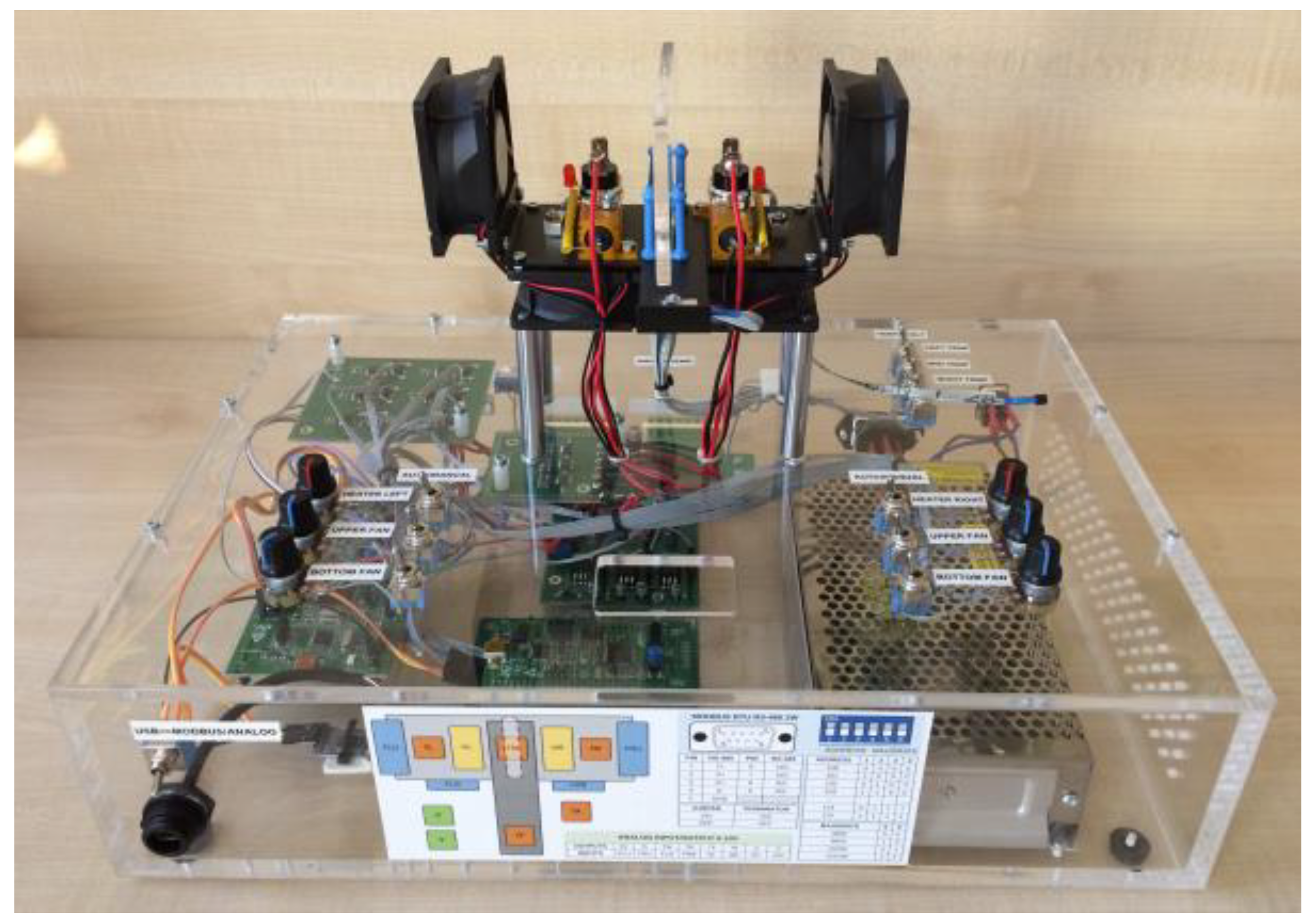
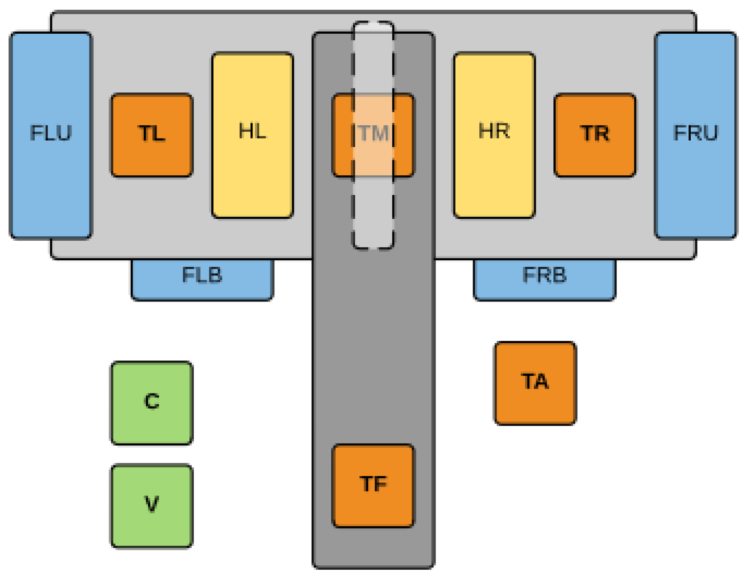
3.3. Laboratory Thermal Stand

The stand is designed as a small process simulator, where the user influences the temperature distribution in the facility through controllable fans and heaters. The bench can be controlled manually or via an automation system using the Modbus communication protocol. A picture of the laboratory thermal stand is presented in Figure 1.

It is an object with six inputs (MV—manipulated variables):

• FLU, FLB, FRU, FRB fans, values from 0 (0% power) to 1000 (100% power),
• HL, HR heaters, values from 0 (0% power) to 1000 (100% power).

There are also seven outputs (PV—process variables):

• TL, TM, TR, TF bench temperature, values from −55.0 °C to +125.0 °C,
• TA ambient temperature, values from −55.0 °C to +125.0 °C,
• C current measurement,
• V voltage measurement.

A PWM (Pulse-Width Modulation) signal controls the actuators. The temperature sensors communicate internally using the OneWire bus, whereas the current and voltage measurements are realized using dedicated electronics. All input and output signals are available via the Modbus protocol. This kind of communication was used during this research project. The schema of the object is presented in Figure 2.

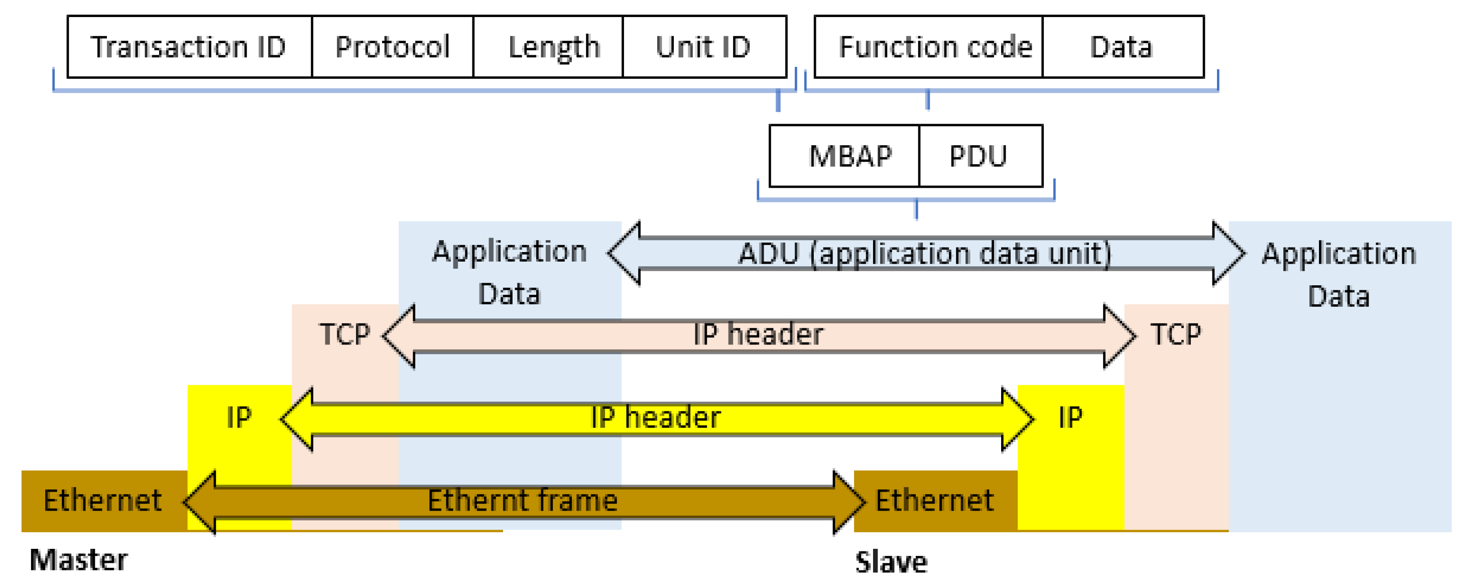
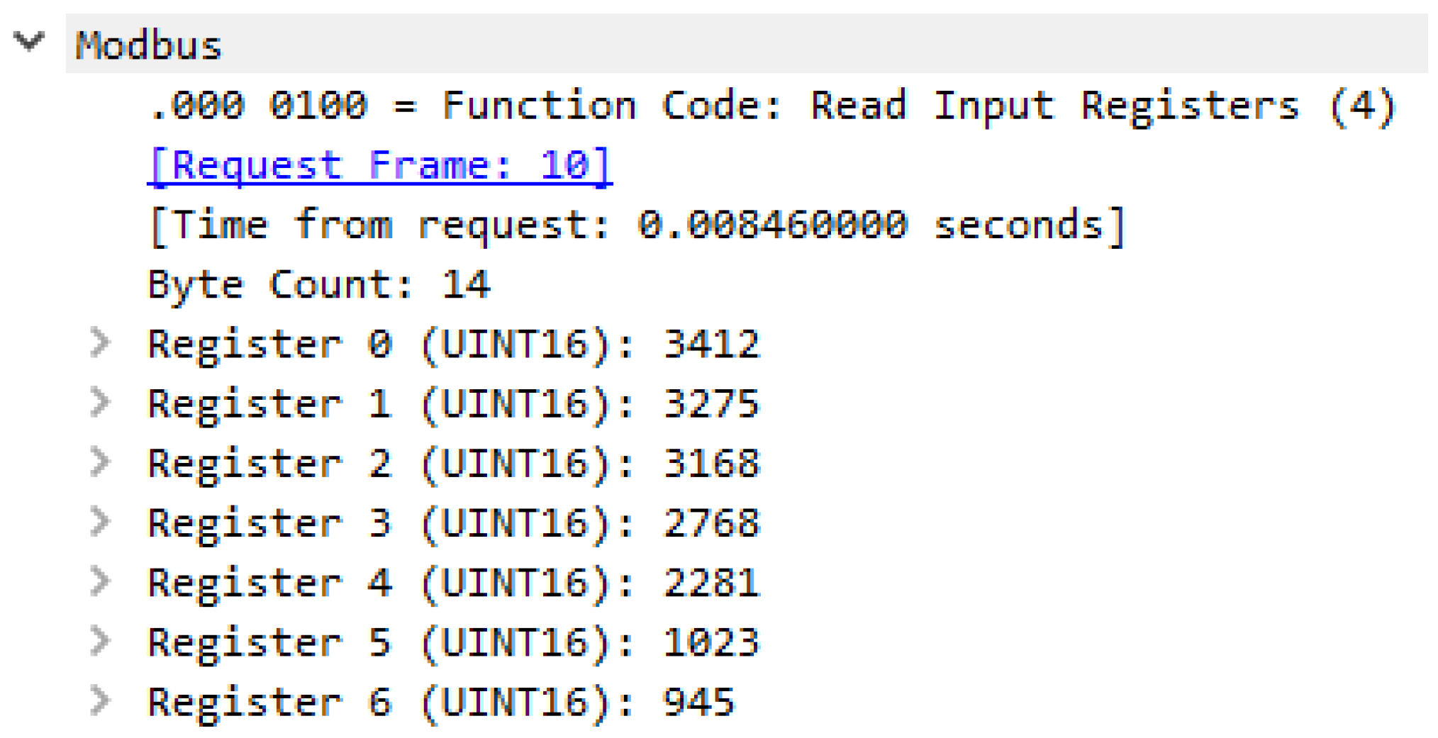
3.4. Modbus Protocol Modbus TCP/IP Data Frame

Figure 3 [29] shows the Modbus TCP/IP communication scheme. This protocol is based on the ETHERNET TCP/IP communication standard. It is equivalent to the Modbus RTU, but it uses the TCP protocol for communication on port 502. It does not have a checksum calculation because the higher TCP layer already implements this.

Modbus TCP/IP is structurally a Modbus RTU protocol with a TCP interface that allows communication over Ethernet. The structure of the Modbus frames determines how data frames are assembled and how they are interpreted, regardless of the medium in which they are transmitted. The Transmission Control Protocol and Internet Protocol (TCP/IP) provide the communication medium for Modbus TCP/IP messages.

Modbus communication begins with a client (master) requesting data from a server (slave). A frame is associated with each message; the meaning of the bits in the frame is explained below [27].

In this paper, we focused on the process data in the frame. A communication example for one channel is presented in Figure 4 and Figure 5.

The MBAP (Modbus Application Protocol Header) contains four fields that define communication rules:

• 2-bytes Transaction Identifier—used by the client to properly pair received responses with requests. This is necessary when multiple messages are sent simultaneously over a TCP link. This value is determined and placed in the request frame by the master, and then it is copied and placed in the response frame.
• 2-bytes Protocol ID—this is always set to 0, and it corresponds with the Modbus protocol designation.
• 2-bytes Message Size—the number of remaining message bytes, which consists of the device ID (Unit ID), function code, and the number of data fields. This field was introduced due to the possibility of splitting a single message into separate TCP/IP packets.
• 1-byte Unit ID—can be relevant, for example, when communicating with Modbus devices equipped with serial interface via gateways (Modbus Data Gateway). In a typical Modbus TCP server application, this field is set to 0 or FF and it is ignored by the server. The server, in its response, duplicates the value received by the client.

Protocol Data Unit (PDU) defines the function code and data/parameters. The function field informs the slave device of the action it is to perform; the data describe the function’s parameters. In response, the function code is duplicated (if the command was executed correctly by the server), and the data contain the required information. In the case of an error, the server can reply with a function code indicating a problem with the execution of the request. It is worth noting that all the data are sent as integer values, which must be considered during prediction and interpretation.

4. Models of Knowledge Discovery

The data transmitted in the communication protocols of the OT networks (e.g., Modbus, Profinet) originate from a physical object and are, therefore, mainly in relationships with each other. The transmitted control values affect the object’s state and the process variables’ values. Consequently, it seems reasonable to assume that building models describing these relationships is possible. As the connections and their nature (static/dynamic relationships) are unknown, models are used during the knowledge discovery process to describe them.

Industrial processes are characterized by working in design areas that are optimized for efficiency. Changes to the operating point, the so-called transient operating state, are carried out infrequently. Therefore, when analyzing process data dependencies and studying static dependencies, full dynamic models can be used.

From the point of view of the future application of the methods in question, the computational complexity is significant. Algorithms placed in the probe must be executed in real-time. Moreover, stability is also important, which will allow selection error levels to eliminate false positive indications.

Many articles discuss the quality and efficiency of machine learning techniques such as the SVM (Support Vector Machine) [30,31,32], RF (Random Forest) [33,34], ELM (Extreme Learning Machine) [35], LSTM (Long Short-Term Memory [36], XGBoost (eXtreme Gradient Boosting) [37,38], CNN (Convolutional Neural Network) [39], and EBM (Explainable Boosting Machine [9]. These algorithms have applications in various domains [11,40,41,42,43]. The general conclusions indicate the superiority of modern methods, such as XGBoost or EBM, over other techniques. In addition, these algorithms have been widely documented and used in cases. XGBoost is particularly noteworthy, which is additionally characterized by the high robustness and stability of the forecast quality—this is very important when using this algorithm in the IDS probe. Therefore, when examining the first approach, XGBoost and EBM were chosen for testing their suitability for possible further implementation in the IDS probe. In the following stages of the research, the authors confronted modern techniques with older approaches and newer, less popular ones (such as LGBM).

4.1. EBM—Explainable Boosting Machines

EBM belongs to the modern group of models that allow very high accuracy while maintaining an understanding of the model structure, which is one of the main problems of neural networks as they do not allow an interpretation of the model parameters. On the other hand, simple regression models are easily interpretable, but are usually low quality. EBM builds upon, or augments, generalized additive models (GAMs) (Equation (1)) [9].

$$g\left(E\left(Y\right)\right)={\beta }_0+f_1\left(x_1\right)+f_2\left(x_2\right)+\cdots +f_n\left(x_n\right)$$

(1)

GAMs are more accurate than simple linear models, and since they do not contain interactions between features, users can also easily interpret them. The EBM has several significant advantages over the generalized additive model (GAM). These advantages pertain to the method of learning as well as the form of the model, which can consider interactions between components (Equation (2)).

$$g\left(E\left[y\right]\right)={\beta }_0+\sum f_i\left(x_i\right)+\sum f_{i,j}\left(x_i{,x}_j\right)$$

(2)

The use of this technique seems promising regarding the task of detecting (describing) dependencies in the process data, about which, nothing is known.

4.2. XGBoost—Extreme Gradient Boosting

Extreme Gradient Boosting (XGBoost) is a method for the implementation of gradient boosting machines, and it is known as one of the best-performing algorithms for supervised learning. It is a decision tree-based machine learning algorithm for classification and regression problems. The Gradient Boosting algorithm builds decision trees sequentially (instead of in parallel and independently, such as Random Forest) so that each successive tree aims to reduce the errors of the previous tree [12].

5. Data

Tests were conducted for the static and dynamic data generated by the simulator and data collected from the real traffic. This approach made it possible to study the properties of the algorithms under different conditions. Simulated data are fully deterministic and uniformly cover the domain. Data from the real object are naturally perturbed and limited to the working areas. Data trends for each case are presented in the following subsections—modeling results and conclusions, in Section 6 and Section 7.

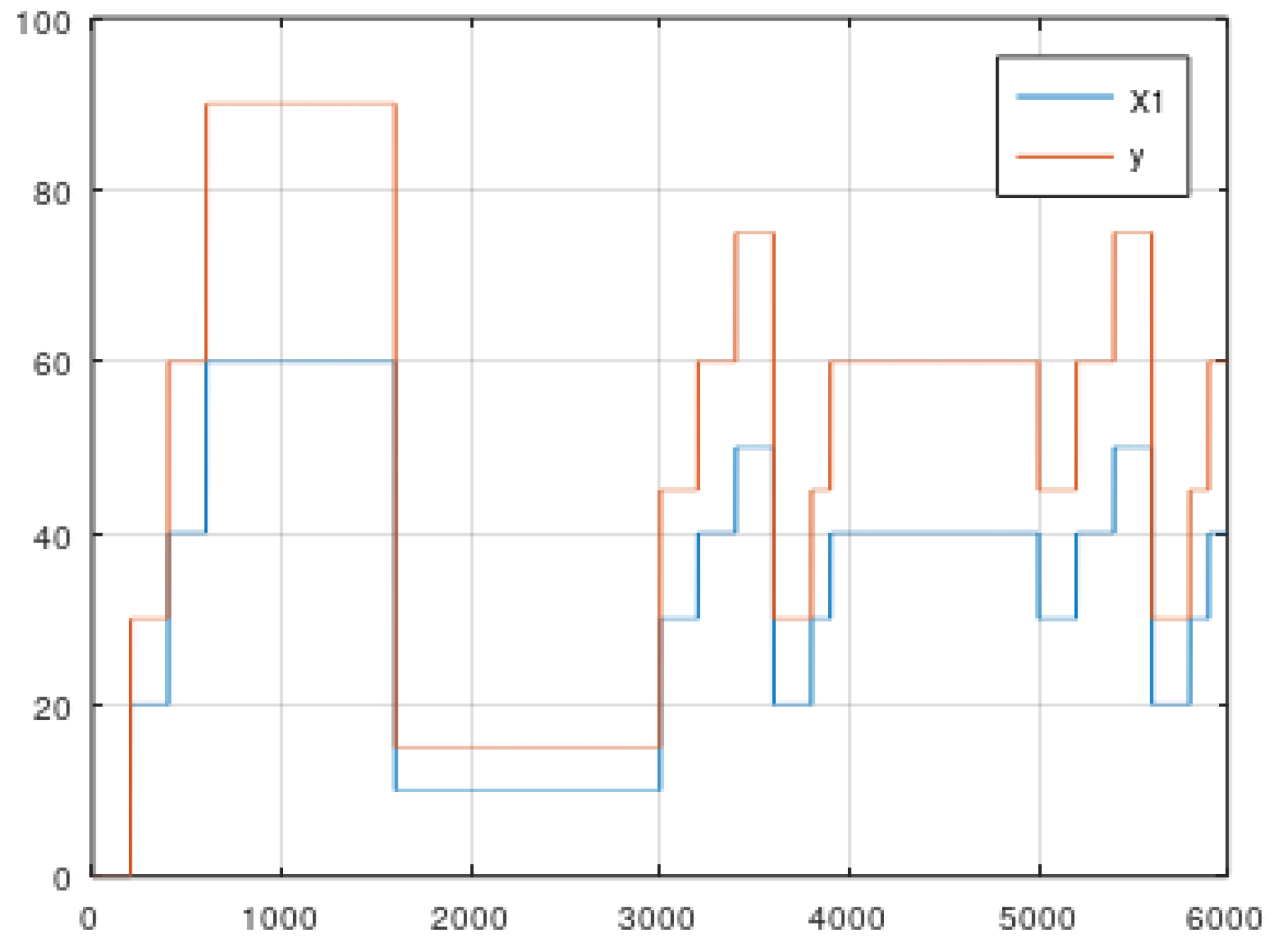
5.1. Static Data from Simulator

Data were collected for several equations. The argument x was a vector of an integer between 1 and 6000. Static data were prepared to test the properties of the learning algorithms in a fully controlled environment.

(a)

Simple linear function (Equations (3) and (4)).

$$X_1=x$$

(3)

$$y=1.5·X_1$$

(4)

Data = [X₁ y] are presented in Figure 6.

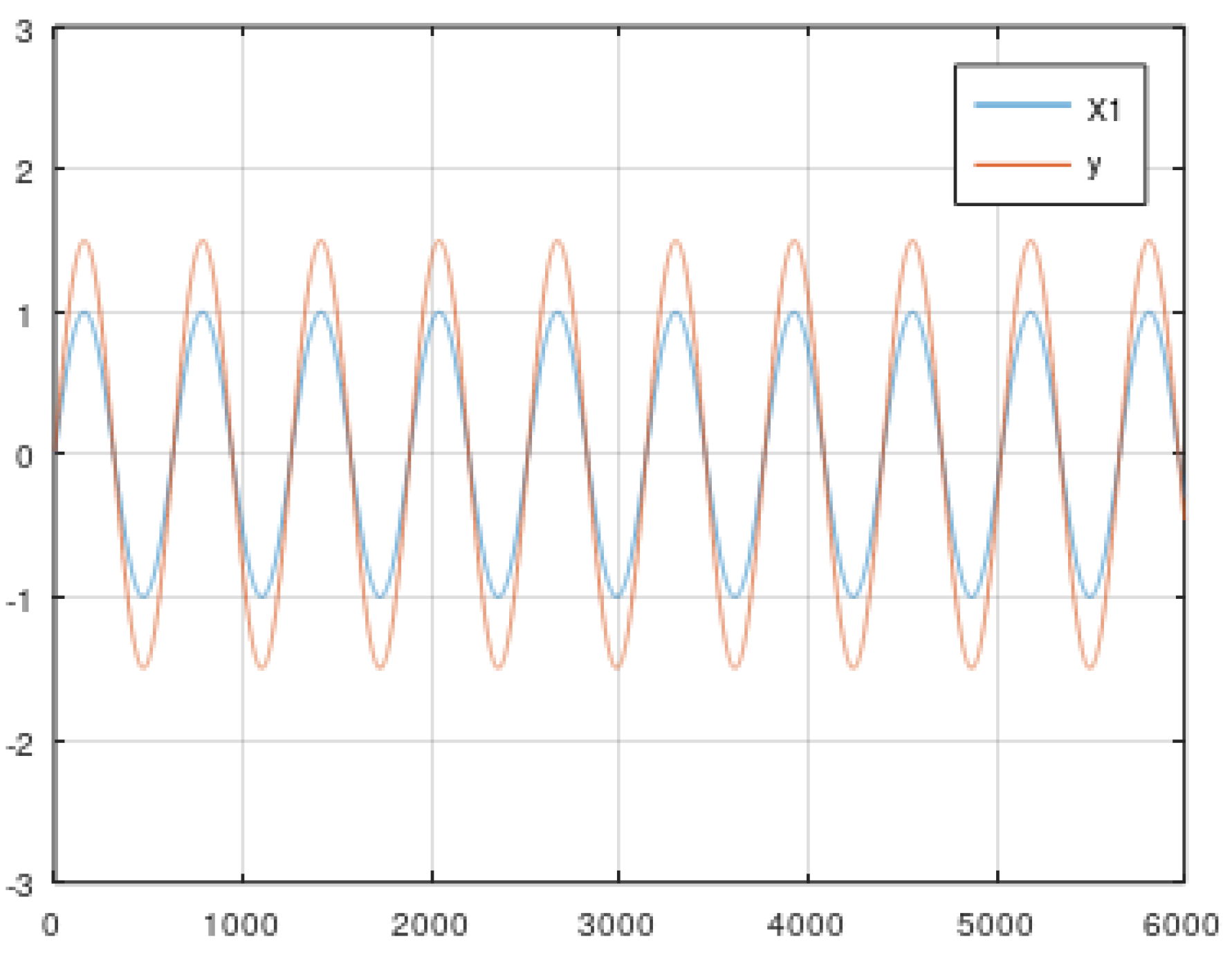
• (b) Rescaled periodic function (Equations (5) and (6)).

$$X_1=\sin (0.01·x)$$

(5)

$$y=1.5·X_1$$

(6)

Data = [X₁ y] are presented in Figure 7.

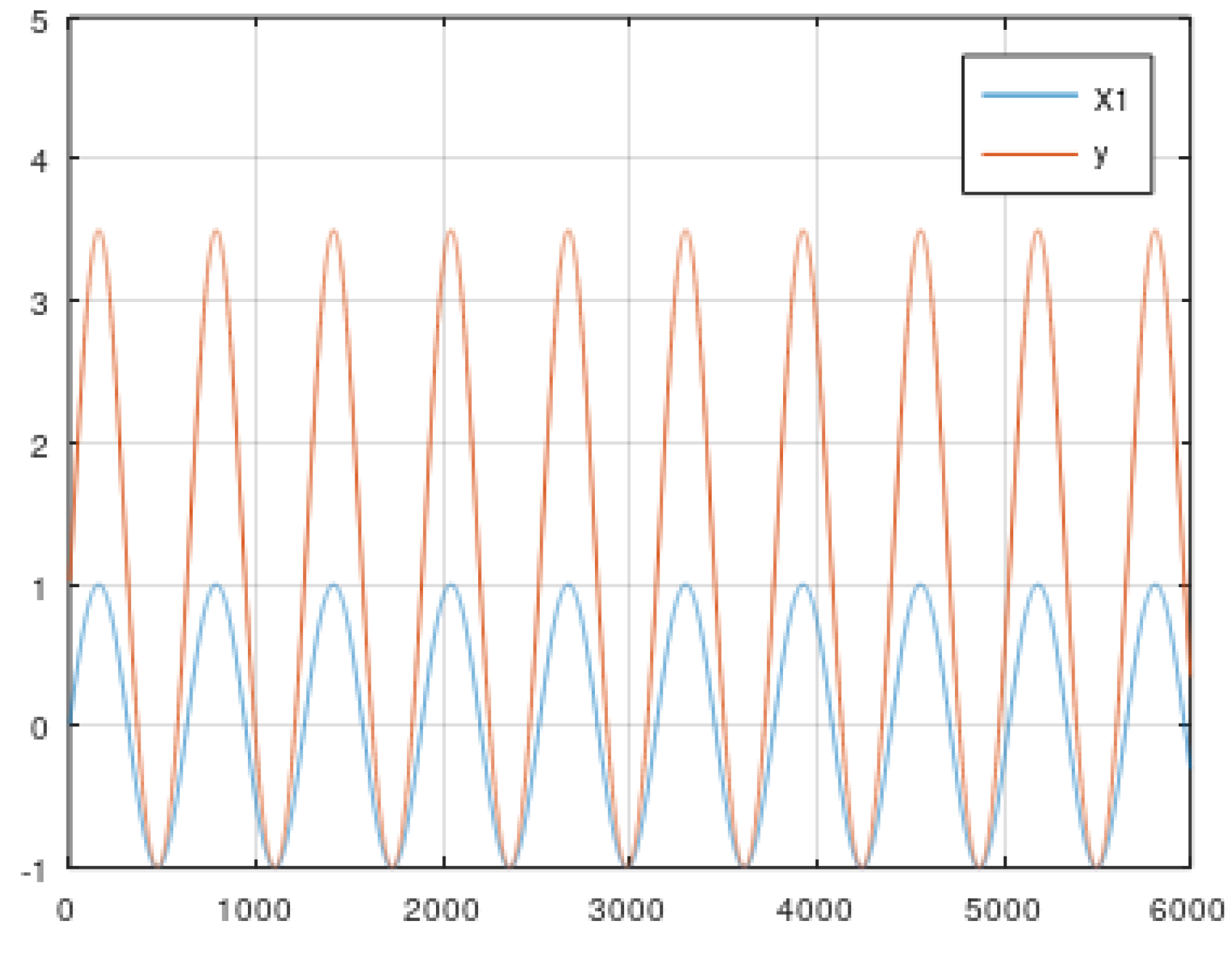
• (c) Composition of a rescaled periodic and power function (Equations (7) and (8)).

$$X_1=\sin (0.01·x)$$

(7)

$$y=1.5·X_1+{X_1}^2$$

(8)

Data = [X₁ y] are presented in Figure 8.

• (d) Composition of a rescaled periodic and modulo function (Equations (9)–(11)).

$$X_1=\mathrm{s}\mathrm{i}\mathrm{n}(0.01·x)$$

(9)

$$X_2=0.01·\mathrm{m}\mathrm{o}\mathrm{d}(x,500)$$

(10)

$$y=1.5·X_1+0.5·X_2$$

(11)

Data = [X₁ X₂ y] are presented in Figure 9.

• (e) Composition of a rescaled periodic, exponential, and modulo function (Equations (12)–(14)).

$$X_1=\mathrm{s}\mathrm{i}\mathrm{n}(0.01·x)$$

(12)

$$X_2=0.01·\mathrm{m}\mathrm{o}\mathrm{d}(x,500)$$

(13)

$$y=1.5·X_1+{X_1}^2-X_2$$

(14)

Data = [X₁ X₂ y] are presented in Figure 10.

• (f) Composition of a rescaled periodic, exponential, modulo, and square root function (Equations (15)–(17)).

$$X_1=\mathrm{s}\mathrm{i}\mathrm{n}(0.01·x)$$

(15)

$$X_2=0.01·\mathrm{m}\mathrm{o}\mathrm{d}(x,500)$$

(16)

$$y=1.5·X_1+{X_1}^2-X_2-\sqrt{X_2}$$

(17)

Data = [X₁ X₂ y] are presented in Figure 11.

5.2. Dynamic Data from the Simulator

Dynamic data were generated using a dynamic model of the heating and cooling laboratory stand. The model was developed using fuzzy set theory to correctly represent the non-linearities in the process. The simulator was limited to four input and two output signals to check the models’ properties under simplified conditions.

The built simulator calculates the left and right temperatures (TL and TR). The signal of the fans, which changes the dynamics and amplifies the effect of the heaters, was used as a fuzzy signal. HL (Heater Left) and HR (Heater Right) and the upper left and right fans FLU (Fan Left Upper) and FRU (Fun Right Upper) were used as modeling signals. Trends of six signals Data = [HL HR FLU FRU TL TR] are presented in Figure 12.

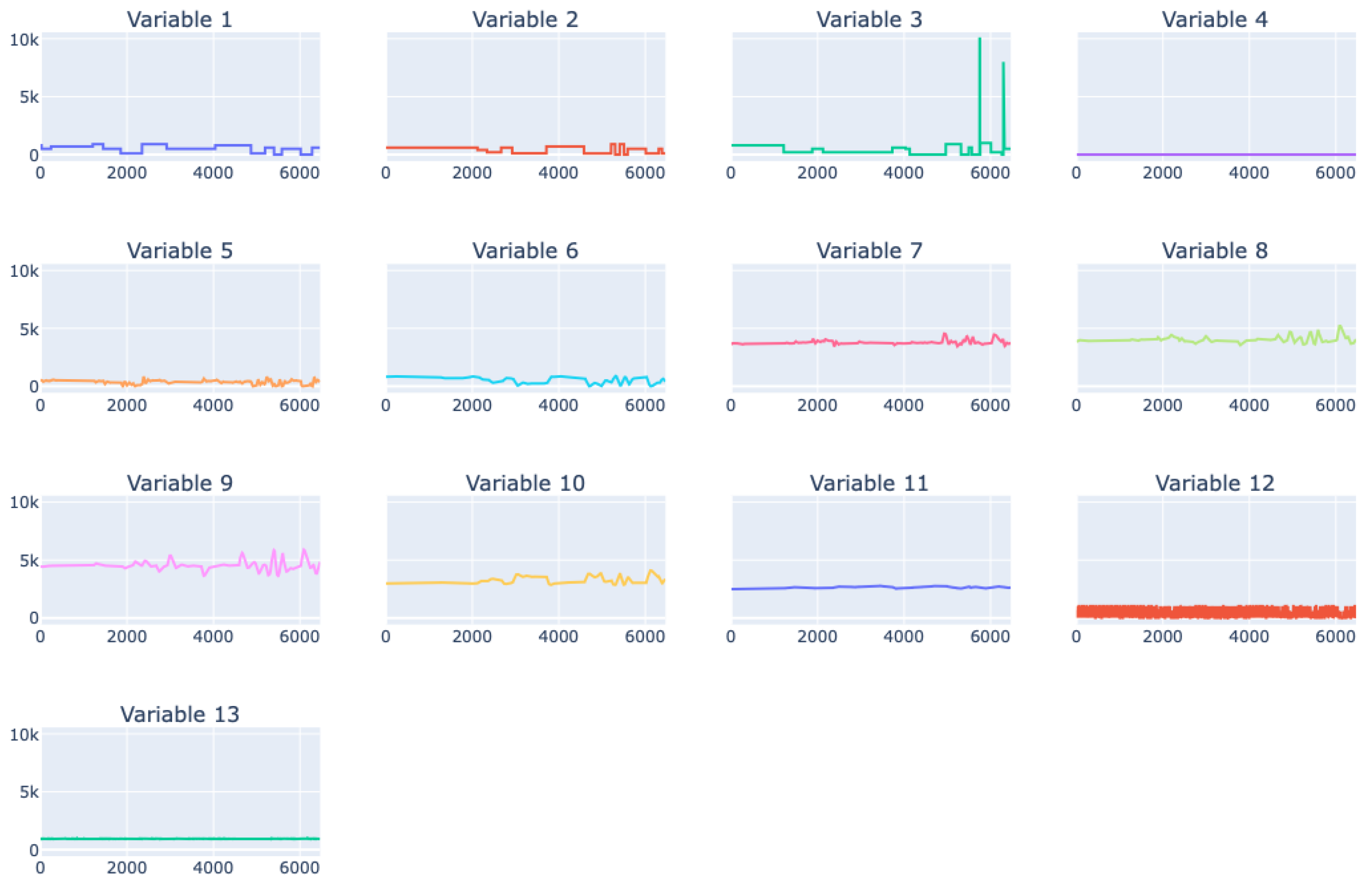
5.3. Real Data from Physical Bench Working in Network

Data were collected from the operation of the stand. Six variables were sent to the bench: control of the left and right heaters, control of the left bottom and upper, and right bottom and upper fans. Seven process variables were read: five temperatures, current, and power.

During the tests, the values of all thirteen variables were read directly from the communication protocol. The trends are shown in Figure 13.

6. Modeling Results

The sets of data described in Section 5 were used for testing XGBoost and EBM algorithms. The trend in blue labeled ‘ground truth’ represents the actual value, and the trend in red represents the prediction. The data was split into training data (the first 90%) and verification data (the last 10%). The learning was performed on a training set using cross-validation. We used Time Series cross-validation, a variation of the classical k-fold cross-validation. Tuning parameters were optimized on the grid. For the XGBoost algorithm we used:

• min child weight: 1, 5, 10,
• gamma: 0.5, 1, 1.5, 2, 5,
• subsample: 0.6, 0.8, 1.0,
• max depth: 3, 4, 5.

For EBM algorithm we used the following parameters:

• learning rate: 0.001, 0.005, 0.01, 0.03,
• interactions: 5, 10, 15,
• max interaction bins: 10, 15, 20,
• min samples leaf: 2, 3, 5,
• max leaves: 3, 5, 10.

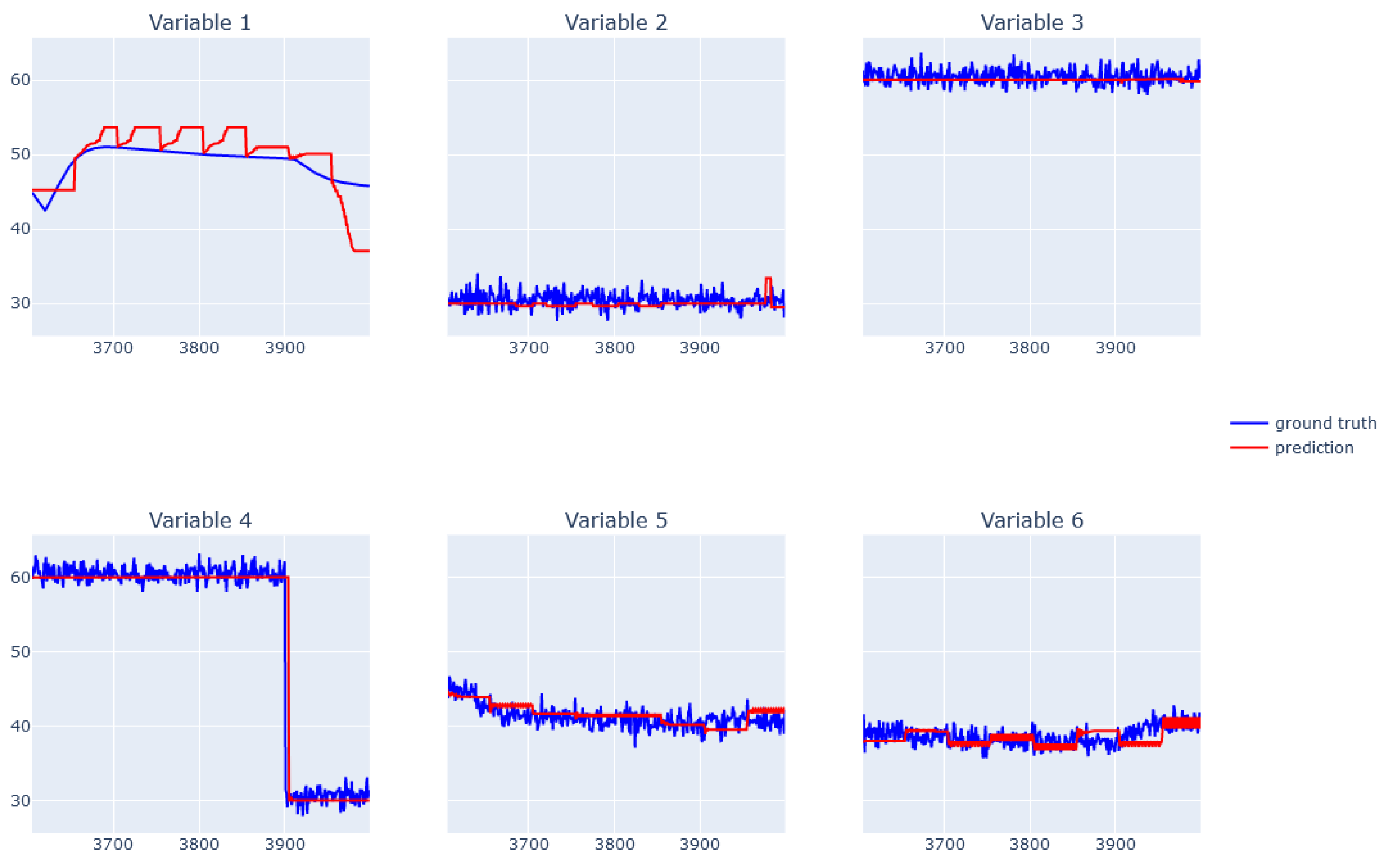
6.1. XGBoost for Static Data from Simulator

The actual (blue line “ground truth”) and predicted (red line) trends for simple linear functions are illustrated in Figure 14. The algorithm was run with the following tuning parameters: gamma = 0.5, max depth = 3, min child weight = 1, and subsample = 1.0. The mean square error was 0.000027.

The actual and predicted trends for the rescaled periodic functions are illustrated in Figure 15. The algorithm was run with the following tuning parameters: gamma = 0.5, max depth = 3, min child weight = 1, and subsample = 1.0. The mean square error was 0.000253.

The actual and predicted trends for the composition of a rescaled periodic and power function are illustrated in Figure 16. The algorithm was run with the following tuning parameters: gamma = 0.5, max depth = 4, min child weight = 1, and subsample = 1.0. The mean square error was 0.000249.

The actual and predicted trends for the composition of a rescaled periodic and modulo function are illustrated in Figure 17. The algorithm was run with the following tuning parameters: gamma = 0.5, max depth = 5, min child weight = 10, and subsample = 1.0. The mean square error was 0.001332.

The actual and predicted trends for the composition of a rescaled periodic, exponential, and modulo function are illustrated in Figure 18. The algorithm was run with the following tuning parameters: gamma = 0.5, max depth = 4, min child weight = 10, and subsample = 1.0. The mean square error was 0.002053.

The actual and predicted trends for the composition of a rescaled periodic, exponential, modulo, and square root function are illustrated in Figure 19. The algorithm was run with the following tuning parameters: gamma = 0.5, max depth = 4, min child weight = 5, and subsample = 1.0. The mean square error was 0.004897.

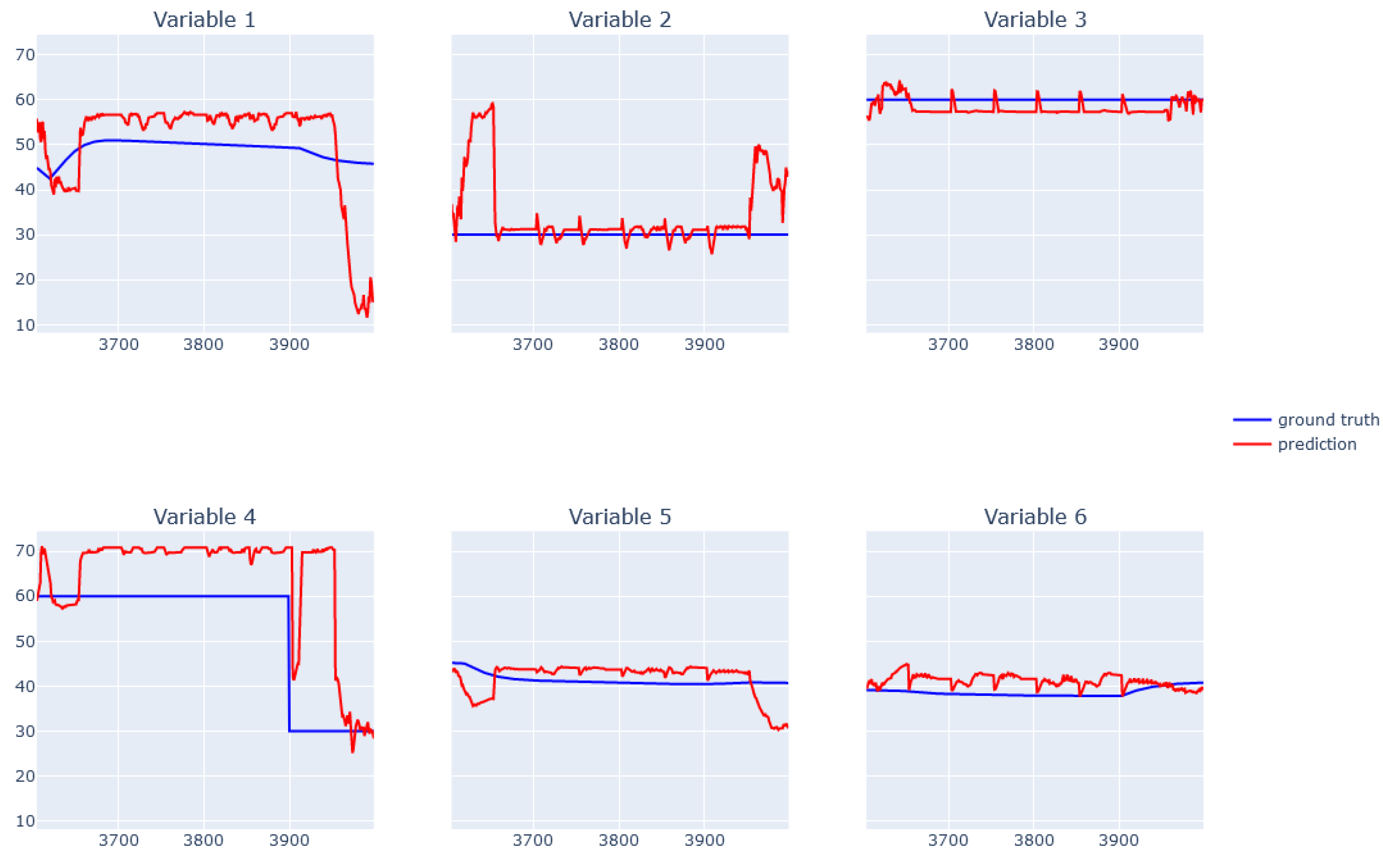
6.2. EBM for Static Data from Simulator

The actual and predicted trends for simple linear functions are illustrated in Figure 20. The algorithm was run with the following tuning parameters: interactions = 5, learning rate = 0.03, max interactions bins = 10, max leaves = 3, min samples leaf = 2. The mean square error was 8.349222 × 10⁻⁷.

The actual and predicted trends for rescaled periodic functions are illustrated in Figure 21. The algorithm was run with the following tuning parameters: interactions = 5, learning rate = 0.03, max interactions bins = 10, max leaves = 10, min samples leaf = 2. The mean square error was 1.754245 × 10⁻⁵.

The actual and predicted trends for the composition of a rescaled periodic and power function are illustrated in Figure 22. The algorithm was run with the following tuning parameters: interactions = 5, learning rate = 0.03, max interactions bins = 10, max leaves = 10, min samples leaf = 3. The mean square error was 3.186037 × 10⁻⁵.

The actual and predicted trends for the composition of a rescaled periodic and modulo function are illustrated in Figure 23. The algorithm was run with the following tuning parameters: interactions = 5, learning rate = 0.03, max interactions bins = 20, max leaves = 3, min samples leaf = 3. The mean square error was 2.998733 × 10⁻⁴.

The actual and predicted trends for the composition of a rescaled periodic, exponential, and modulo function are illustrated in Figure 24. The algorithm was run with the following tuning parameters: interactions = 5, learning rate = 0.03, max interactions bins = 15, max leaves = 3, min samples leaf = 2. The mean square error was 7.806904 × 10⁻⁴.

The actual and predicted trends for the composition of a rescaled periodic, exponential, modulo, and square root function are illustrated in Figure 25. The algorithm was run with the following tuning parameters: interactions = 5, learning rate = 0.03, max interactions bins = 10, max leaves = 5, min samples leaf = 2. The mean square error was 9.588033 × 10⁻⁴.

The prediction results obtained for both algorithms were excellent. Naturally, the quality of the prediction deteriorated as the function’s complexity increases. In the case of the XGBoost algorithm, the mean square error of the first function was 0.000027, and for the last, most complex function, it was 0.004897 (i.e., a value that was almost 200 times worse). For the EBM algorithm, the mean square error of the first function was 8.349222 × 10⁻⁷, and for the last function, it was 9.588033 × 10⁻⁴, which was a value that was more than 1000 times worse. The prediction error obtained for the EBM algorithm was about 100 times lower than for the XGBoost algorithm.

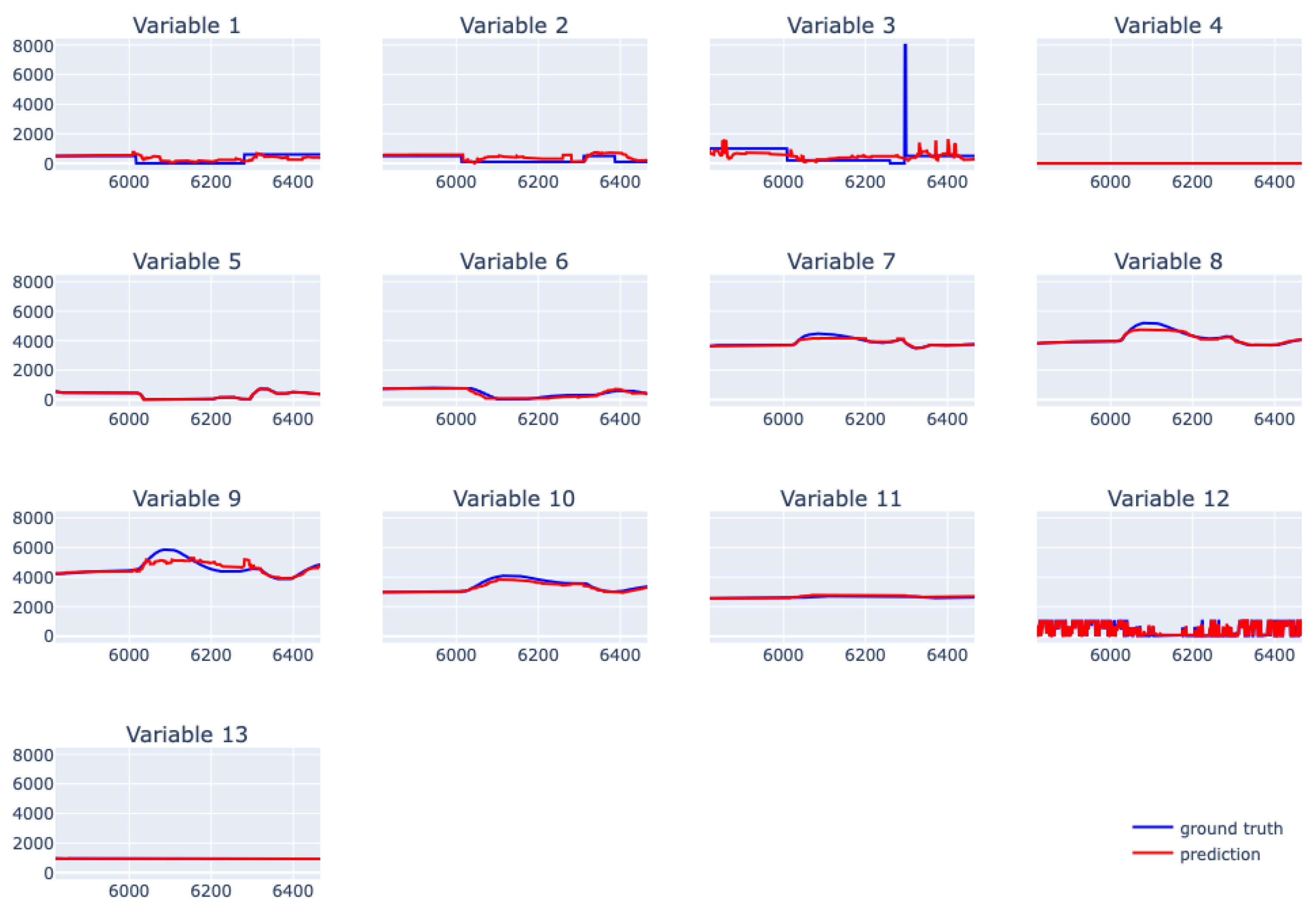
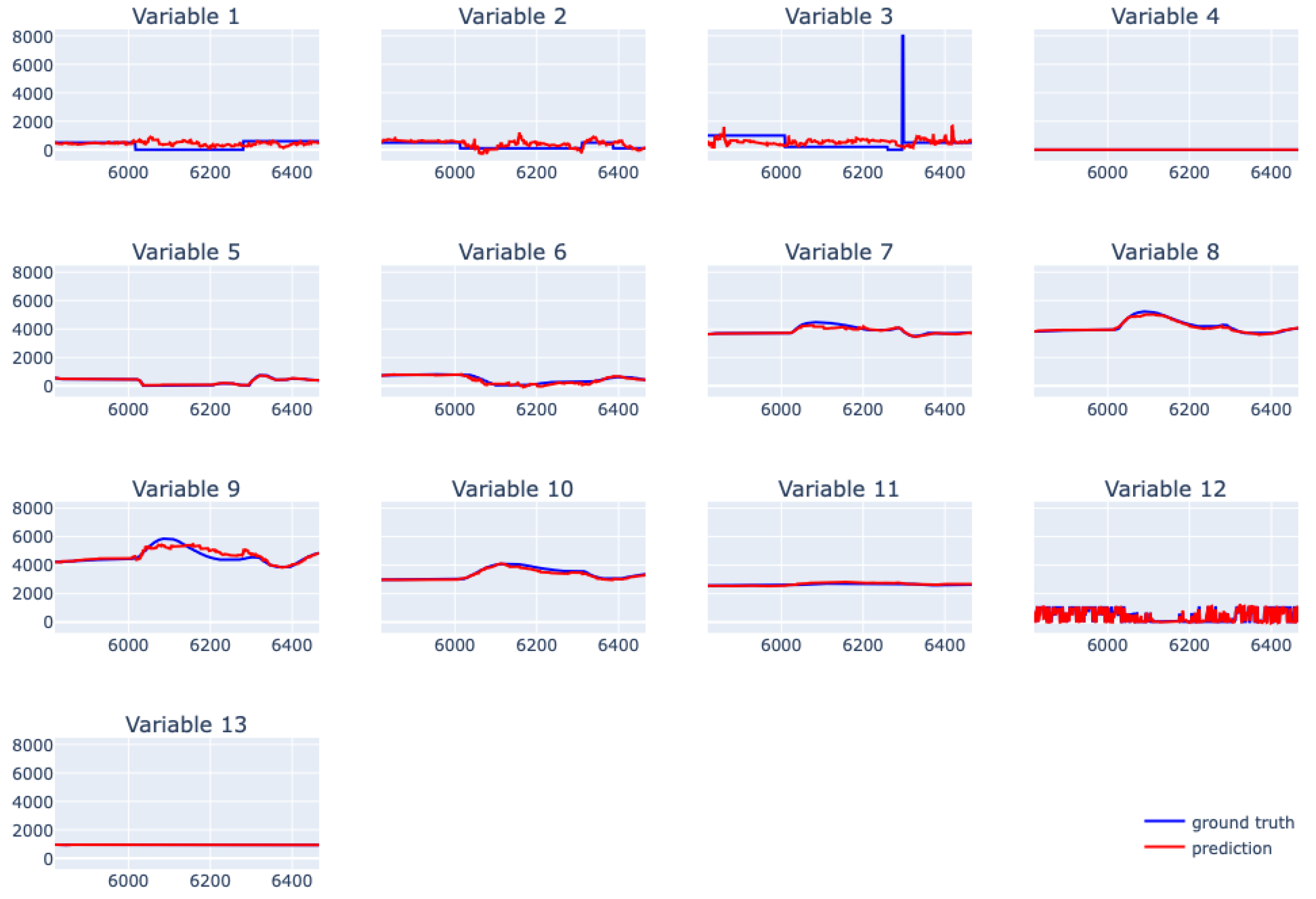
6.3. XGBoost for Dynamic Data from Simulator

During the study, it was assumed that the relationship between the signals was unknown, particularly those related to the inputs and outputs. Therefore, it was assumed that all signals were modeled independently. Figure 26 shows the modeling results, with the last 10% of the samples from all data used as the verification set. The values of the used tuning parameters are presented in

Table 1. XGBoost algorithm parameters for the dynamic data from the simulator.

Variable	Gamma	Max Depth	Min Child Weight	Subsample
1	0.5	3	10	0.6
2	2	5	1	0.6
3	5	5	5	0.6
4	0.5	3	5	0.6
5	0.5	3	1	1.0
6	0.5	4	1	1.0

.

The worst results were obtained for variable 1; this is the correct result as this variable is the input variable (i.e., the explanatory variable). The output variables (i.e., the explanatory variables) are variables 5 and 6, for which the predicted values reflect the actual values with reasonably high accuracy.

To test the algorithm’s robustness, an attempt was made to introduce an additive disturbance to the output variables, and the noisy waveforms are shown in Figure 27.

The introduction of noise did not affect the behavior of the forecasting algorithm. The resultant forecasts are still high, as shown in Figure 28.

Introducing additional noise on variables 2, 3, and 4 also did not affect the behavior of the prediction algorithm, as shown in Figure 29.

6.4. EBM for Dynamic Data from Simulator

An analogous study for the simulator data was carried out using the EBM model. In this case, the results (Figure 30) were significantly worse. The values of the used tuning parameters are presented in

Table 2. EBM algorithm parameters for the dynamic data from the simulator.

Variable	Interactions	Learning Rate	Max Interactions Bins	Max Leaves	Min Samples Leaf
1	5	0.03	10	3	2
2	5	0.03	20	3	2
3	5	0.03	20	3	2
4	5	0.03	10	5	2
5	5	0.03	15	3	2
6	5	0.03	10	3	2

.

6.5. XGBoost for Real Data from Physical Bench Working in Network

The data collected from the physical site were split into training and verification data (10% of the set) and they were analyzed in the same way as the data described in the previous subsections. The tests were carried out on the dataset described in Section 5.3. The values of the used tuning parameters are presented in

Table 3. XGBoost algorithm parameters for the real data from the physical bench.

Variable	Gamma	Max Depth	Min Child Weight	Subsample
1	0.5	3	10	1
2	0.5	5	1	0.6
3	2	4	10	0.6
4	0.5	3	1	0.8
5	5	3	1	0.6
6	1	3	10	0.6
7	0.5	4	10	0.8
8	5	4	5	0.6
9	2	5	10	0.6
10	5	4	10	0.6
11	1.5	3	5	0.6
12	0.5	3	10	0.6
13	1.5	3	10	0.8

. The trends are shown in Figure 31, and the RMSE results are shown in

Table 4. RMSE factor for the results from the XGBoost algorithm.

Variable	RMSE
1	230.400962
2	349.570717
3	604.089026
4	0.000013
5	28.216980
6	92.831780
7	105.422982
8	152.271105
9	300.535097
10	147.651014
11	40.982248
12	107.979691
13	4.392808

.

The data collected from the actual movement is characterized by higher variability, which is reflected by the incorrectly modeled inputs in the process (especially variables: 0, 1, and 2). As with the simulator, the process outputs (variables 7 through 13) provided much better predictions than the process inputs.

6.6. EBM for Real Data from Physical Bench Working in Network

Identical tests were carried out for the EBM algorithm. The values of the used tuning parameters are presented in

Table 5. EBM algorithm parameters for the real data from the physical bench.

Variable	Interactions	Learning Rate	Max Interactions Bins	Max Leaves	Min Samples Leaf
1	10	0.01	20	3	2
2	10	0.01	20	3	2
3	10	0.01	10	3	2
4	10	0.01	20	3	2
5	10	0.01	10	3	2
6	10	0.01	15	3	2
7	10	0.01	20	3	2
8	10	0.01	20	3	2
9	10	0.01	20	3	2
10	5	0.01	20	3	2
11	10	0.01	15	3	2
12	10	0.01	20	3	2
13	10	0.01	20	3	2

. The results are shown in Figure 32 and

Table 6. RMSE factor for results from XGBoost algorithm.

Variable	RMSE
1	323.577118
2	237.924763
3	675.113722
4	0.000000
5	38.752803
6	96.573082
7	128.493062
8	83.705900
9	277.835994
10	119.786830
11	57.369146
12	121.508004
13	4.637388

.

Very similar results were obtained for the EBM algorithm. Some variables were modeled better, and others worse; no consistent relationship was found. As with XGBoost, the input data from set three were predicted to be worse than the output data. Similar to XGBoost, the EBM model correctly predicted the steady-state data.

7. Conclusions

The mechanisms used in this paper for detecting dependencies in data work well for linear and non-linear data. The developed examples have shown the usefulness of the methods for both one-dimensional and multidimensional data. Better results were obtained with data from static relationships. In the case of dynamic data, the algorithms used to model transient states could be better; for steady states, the accuracy is high.

Improving the quality of dynamic models could be achieved by using model outputs that are measured a few moments earlier as input. As a result, the model would take the form of an autoregressive model. However, this approach has several drawbacks, the primary drawback being the selection of the lag value and the number of previous measurements. In addition, after poisoning the attacked value, after a few steps, such a model may count the forecast using the poisoned value—especially when the attacked value changes slowly.

Examining the communication stream as communication packets, with regard to the level of data transmitted, does not allow for an a priori determination of cause-and-effect relationships between signals, which should be understood as process values. It is impossible to indicate which variables are explanatory and which are response variables. Writing or reading functions that are recognizable at the protocol level do not determine the role of a variable in the process. The algorithms used do not distinguish between the input and output signals. The model assumes that each signal is predicted using all others, thus causing some signals to be significantly less well modeled. This is natural, as reverse causality translates into prediction quality. Therefore, to increase the algorithm’s robustness against false positives, algorithms should be used that eliminate the analysis signals that are physical input variables (i.e., explanatory variables) in the process, as these predictions have low accuracy.

The deep monitoring of the data transmitted in the protocols allows relationships to be recognized and continuously monitored. This mechanism can be used in diagnostic systems to protect against cyberattacks. Detecting relationship changes can indicate a flaw in the installation or an attempted cyberattack on the protocol or device data. The passage of an intruder to the control systems level indicates poor facility protection. Detection of an attack at the data level is a late action; it is the last moment where it is possible to react. Detection of inaccuracies at this stage may indicate that previous attack prevention mechanisms, implemented in accordance with the kill chain concept, have failed. Therefore, any perceived anomalies should be a signal to conduct a security systems audit, a thorough analysis of system logs, and of metrics related to network traffic.

References

1. Wang, D. Building value in a world of technological change: Data analytics and Industry 4.0. IEEE Eng. Manag. Rev. 2018, 46, 32–33. [Google Scholar] [CrossRef]
2. Ancarani, A.; Di Mauro, C. Reshoring and Industry 4.0: How often do they go together? IEEE Eng. Manag. Rev. 2018, 46, 87–96. [Google Scholar] [CrossRef]
3. Sony, M.; Naik, S.S. Ten lessons for managers while implementing Industry 4.0. IEEE Eng. Manag. Rev. 2019, 47, 45–52. [Google Scholar] [CrossRef]
4. Malik, A.K.; Emmanuel, N.; Zafar, S.; Khattak, H.A.; Raza, B.; Khan, S.; Al-Bayatti, A.H.; Alassafi, M.O.; Alfakeeh, A.S.; Alqarni, M.A. From Conventional to State-of-the-Art IoT Access Control Models. Electronics 2020, 9, 1693. [Google Scholar] [CrossRef]
5. Zafar, F.; Khan, A.; Anjum, A.; Maple, C.; Shah, M.A. Location Proof Systems for Smart Internet of Things: Requirements, Taxonomy, and Comparative Analysis. Electronics 2020, 9, 1776. [Google Scholar] [CrossRef]
6. Knapp, E.D.; Langill, J.T. Industrial Network Security Securing Critical Infrastructure Networks for Smart Grid, SCADA, and Other Industrial Control Systems; Elsevier: Amsterdam, The Netherlands, 2015. [Google Scholar]
7. SP 800-82 Rev. 2; Guide to Industrial Control Systems (ICS) Security. National Institute of Standards and Technology: Gaithersburg, MD, USA, 2015.
8. ISA-99.00.01; Security for Industrial Automation and Control Systems—Part 1: Terminology, Concepts and Models. American National Standard: Washington, DC, USA, 2007.
9. Tsiknas, K.; Taketzis, D.; Demertzis, K.; Skianis, C. Cyber Threats to Industrial IoT: A Survey on Attacks and Countermeasures. IoT 2021, 2, 163–186. [Google Scholar] [CrossRef]
10. Inayat, U.; Zia, M.F.; Mahmood, S.; Khalid, H.M.; Benbouzid, M. Learning-Based Methods for Cyber Attacks Detection in IoT Systems: A Survey on Methods, Analysis, and Future Prospects. Electronics 2022, 11, 1502. [Google Scholar] [CrossRef]
11. Maxwell, A.E.; Sharma, M.; Donaldson, K.A. Explainable Boosting Machines for Slope Failure Spatial Predictive Modeling. Remote Sens. 2021, 13, 4991. [Google Scholar] [CrossRef]
12. Chen, T.; Guestrin, C. XGBoost: A Scalable Tree Boosting System. In Proceedings of the 22nd ACM SIGKDD International Conference on Knowledge Discovery and Data Mining, San Francisco, CA, USA, 13–17 August 2016; pp. 785–794. [Google Scholar]
13. Slammer Worm and David-Besse Nuclear Plant. 2015. Available online: http://large.stanford.edu/courses/2015/ph241/holloway2/ (accessed on 20 October 2021).
14. Neubert, T.; Claus Vielhauer, C. Kill Chain Attack Modelling for Hidden Channel Attack Scenarios in Industrial Control Systems. IFAC-PapersOnLine 2020, 53, 11074–11080. [Google Scholar] [CrossRef]
15. Nourian, A.; Madnick, S. A systems theoretic approach to the security threats in cyber physical systems applied to stuxnet. IEEE Trans. Dependable Secur. Comput. 2015, 15, 2–13. [Google Scholar] [CrossRef]
16. Chen, T. Stuxnet, the real start of cyber warfare? IEEE Netw. 2010, 24, 2–3. [Google Scholar]
17. Lee, R.M.; Assante, M.J.; Conway, T. German steel mill cyberattack. Ind. Control Syst. 2014, 30, 62. [Google Scholar]
18. Xiang, Y.; Wang, L.; Liu, N. Coordinated attacks on electric power systems in a cyber-physical environment. Electr. Power Syst. Res. 2017, 149, 156–168. [Google Scholar] [CrossRef]
19. Yang, D.; Usynin, A.; Hines, J. Anomaly-based intrusion detection for SCADA systems. In Proceedings of the Fifth International Topical Meeting on Nuclear Plant Instrumentation, Control and Human–Machine Interface Technologies, Albuquerque, NM, USA, 12–16 November 2006; pp. 12–16. Available online: https://citeseerx.ist.psu.edu/document?repid=rep1&type=pdf&doi=1af84c9c62fb85590c41b7cfc9357919747842b2 (accessed on 10 February 2023).
20. Tsang, C.; Kwong, S. Multi-agent intrusion detection system for an industrial network using ant colony clustering approach and unsupervised feature extraction. In Proceedings of the IEEE International Conference on Industrial Technology, Hong Kong, China, 14–17 December 2005; pp. 51–56. [Google Scholar]
21. Gao, W.; Morris, T.; Reaves, B.; Richey, D. On SCADA control system command and response injection and intrusion detection. In Proceedings of the eCrime Researchers Summit, Dallas, TX, USA, 18–20 October 2010; pp. 1–9. [Google Scholar]
22. Digital Bond, Modbus TCP Rules, Sunrise, Florida. Available online: www.digitalbond.com/tools/quickdraw/modbus-tcp-rules (accessed on 10 February 2023).
23. Javadpour, A.; Wang, G. cTMvSDN: Improving resource management using combination of Markov-process and TDMA in software-defined networking. J. Supercomput. 2021, 78, 3477–3499. [Google Scholar] [CrossRef]
24. Naess, E.; Frincke, D.; McKinnon, A.; Bakken, D. Configurable middleware-level intrusion detection for embedded systems. In Proceedings of the Twenty-Fifth IEEE International Conference on Distributed Computing Systems, Columbus, OH, USA, 6–10 June 2005; pp. 144–151. [Google Scholar]
25. Valdes, A.; Cheung, S. Communication pattern anomaly detection in process control systems. In Proceedings of the IEEE Conference on Technologies for Homeland Security, Waltham, MA, USA, 11–12 May 2009; pp. 22–29. [Google Scholar]
26. Valdes, A.; Cheung, S. Intrusion monitoring in process control systems. In Proceedings of the Forty-Second Hawaii International Conference on System Sciences, Waikoloa, HI, USA, 5–8 January 2009. [Google Scholar]
27. Roesch, M. Snort—Lightweight intrusion detection for networks. In Proceedings of the Thirteenth USENIX Conference on System Administration, Seattle, WA, USA, 7–12 December 1999; pp. 226–238. [Google Scholar]
28. Alshammari, A.; Aldribi, A. Apply machine learning techniques to detect malicious network traffic in cloud computing. J. Big Data 2021, 8, 90. [Google Scholar] [CrossRef]
29. Smolarczyk, M.; Plamowski, S.; Pawluk, J.; Szczypiorski, K. Anomaly Detection in Cyclic Communication in OT Protocols. Energies 2022, 15, 1517. [Google Scholar] [CrossRef]
30. Jędrzejczyk, A.; Firek, K.; Rusek, J. Convolutional Neural Network and Support Vector Machine for Prediction of Damage Intensity to Multi-Storey Prefabricated RC Buildings. Energies 2022, 15, 4736. [Google Scholar] [CrossRef]
31. Najwa Mohd Rizal, N.; Hayder, G.; Mnzool, M.; Elnaim, B.M.E.; Mohammed, A.O.Y.; Khayyat, M.M. Comparison between Regression Models, Support Vector Machine (SVM), and Artificial Neural Network (ANN) in River Water Quality Prediction. Processes 2022, 10, 1652. [Google Scholar] [CrossRef]
32. Adugna, T.; Xu, W.; Fan, J. Comparison of Random Forest and Support Vector Machine Classifiers for Regional Land Cover Mapping Using Coarse Resolution FY-3C Images. Remote Sens. 2022, 14, 574. [Google Scholar] [CrossRef]
33. Nhu, V.-H.; Zandi, D.; Shahabi, H.; Chapi, K.; Shirzadi, A.; Al-Ansari, N.; Singh, S.K.; Dou, J.; Nguyen, H. Comparison of Support Vector Machine, Bayesian Logistic Regression, and Alternating Decision Tree Algorithms for Shallow Landslide Susceptibility Mapping along a Mountainous Road in the West of Iran. Appl. Sci. 2020, 10, 5047. [Google Scholar] [CrossRef]
34. Dabija, A.; Kluczek, M.; Zagajewski, B.; Raczko, E.; Kycko, M.; Al-Sulttani, A.H.; Tardà, A.; Pineda, L.; Corbera, J. Comparison of Support Vector Machines and Random Forests for Corine Land Cover Mapping. Remote Sens. 2021, 13, 777. [Google Scholar] [CrossRef]
35. Rath, S.K.; Sahu, M.; Das, S.P.; Bisoy, S.K.; Sain, M. A Comparative Analysis of SVM and ELM Classification on Software Reliability Prediction Model. Electronics 2022, 11, 2707. [Google Scholar] [CrossRef]
36. Shin, S.-Y.; Woo, H.-G. Energy Consumption Forecasting in Korea Using Machine Learning Algorithms. Energies 2022, 15, 4880. [Google Scholar] [CrossRef]
37. Jafari, S.; Shahbazi, Z.; Byun, Y.-C. Lithium-Ion Battery Health Prediction on Hybrid Vehicles Using Machine Learning Approach. Energies 2022, 15, 4753. [Google Scholar] [CrossRef]
38. Yang, S.; Wu, J.; Du, Y.; He, Y.; Chen, X. Ensemble learning for short-term traffic prediction based on gradient boosting machine. J. Sens. 2017, 2017, 7074143. [Google Scholar] [CrossRef]
39. Shahbazi, Z.; Byun, Y.C. Computing focus time of paragraph using deep learning. In Proceedings of the 2019 IEEE Transportation Electrification Conference and Expo, Asia-Pacific (ITEC Asia-Pacific), Seogwipo, Republic of Korea, 8–10 May 2019; pp. 1–4. [Google Scholar]
40. Shahbazi, Z.; Byun, Y.C. LDA Topic Generalization on Museum Collections. In Smart Technologies in Data Science and Communication; Springer: Singapore, 2020; pp. 91–98. [Google Scholar]
41. Shahbazi, Z.; Byun, Y.C.; Lee, D.C. Toward representing automatic knowledge discovery from social media contents based on document classification. Int. J. Adv. Sci. Technol. 2020, 29, 14089–14096. [Google Scholar]
42. Shahbazi, Z.; Byun, Y.C. Topic prediction and knowledge discovery based on integrated topic modeling and deep neural networks approaches. J. Intell. Fuzzy Syst. 2021, 41, 2441–2457. [Google Scholar] [CrossRef]
43. Walters, B.; Ortega-Martorell, S.; Olier, I.; Lisboa, P.J.G. How to Open a Black Box Classifier for Tabular Data. Algorithms 2023, 16, 181. [Google Scholar] [CrossRef]
Figure 1. Laboratory thermal stand.
Energies 16 04056 g001
Figure 2. Laboratory thermal stand schema.
Energies 16 04056 g002
Figure 3. Modbus TCP/IP ADU (Application Data Unit).
Energies 16 04056 g003
Figure 4. Example of writing six values.
Energies 16 04056 g004
Figure 5. Example of reading seven values.
Energies 16 04056 g005
Figure 6. Simple linear function data.
Energies 16 04056 g006
Figure 7. Rescaled periodic function data.
Energies 16 04056 g007
Figure 8. Composition of rescaled periodic and power function data.
Energies 16 04056 g008
Figure 9. Composition of rescaled periodic and modulo function data.
Energies 16 04056 g009
Figure 10. Composition of rescaled periodic, exponential, and modulo function data.
Energies 16 04056 g010
Figure 11. Composition of rescaled periodic, exponential, modulo, and square root function data.
Energies 16 04056 g011
Figure 12. Data from the dynamic simulator.
Energies 16 04056 g012
Figure 13. Data from laboratory bench.
Energies 16 04056 g013
Figure 14. Actual and XGBoost predicted trends for simple linear function.
Energies 16 04056 g014
Figure 15. Actual and XGBoost predicted trends for rescaled periodic function.
Energies 16 04056 g015
Figure 16. Actual and XGBoost predicted trends for rescaled periodic and power function composition.
Energies 16 04056 g016
Figure 17. Actual and XGBoost predicted trends for rescaled periodic and modulo function composition.
Energies 16 04056 g017
Figure 18. Actual and XGBoost predicted trends for rescaled periodic, exponential, and modulo function composition.
Energies 16 04056 g018
Figure 19. Actual and XGBoost predicted trends for rescaled periodic, exponential, modulo, and square root function composition.
Energies 16 04056 g019
Figure 20. Actual and EBM predicted trends for simple linear function.
Energies 16 04056 g020
Figure 21. Actual and EBM predicted trends for rescaled periodic function.
Energies 16 04056 g021
Figure 22. Actual and EBM predicted trends for rescaled periodic and power function composition.
Energies 16 04056 g022
Figure 23. Actual and EBM predicted trends for rescaled periodic and modulo function composition.
Energies 16 04056 g023
Figure 24. Actual and EBM predicted trends for rescaled periodic, exponential, and modulo function composition.
Energies 16 04056 g024
Figure 25. Actual and EBM predicted trends for rescaled periodic, exponential, modulo, and square root function composition.
Energies 16 04056 g025
Figure 26. Modeling results from the XGBoost algorithm for the dynamic data from the simulator.
Energies 16 04056 g026
Figure 27. Dynamic data from the simulator—noise added to variables five and six.
Energies 16 04056 g027
Figure 28. Modeling results from the XGBoost algorithm for dynamic data from simulator—noise added to variables 5 and 6.
Energies 16 04056 g028
Figure 29. Modeling results from the XGBoost algorithm for the dynamic data from the simulator—noise added to variables: 2, 3, and 4.
Energies 16 04056 g029
Figure 30. Modeling results from the EBM algorithm for the dynamic data from the simulator.
Energies 16 04056 g030
Figure 31. Modeling results from the XGBoost algorithm for the dynamic data from the laboratory stage.
Energies 16 04056 g031
Figure 32. Modeling results from the EBM algorithm for the dynamic data from the laboratory stage.
Energies 16 04056 g032