Abstract
This paper presents an estimation of the parameters for a Double Layer Super Capacitor (DLC) that is modelled with a two-branch circuit. The estimation is achieved using a constrained minimization technique, which is developed off-line and uses a single constraint to write the matrix equation. The model is algebraically manipulated to obtain a matrix equation, and a signal processing system is developed to prepare the signals for the identification algorithms. The proposed method builds on the results obtained using an unconstrained ordinary least-squares (OLS) technique. The method is tested both in simulation and experimentally, using a specially-designed experimental rig. A current ramp input is used to generate the corresponding output voltage and its derivatives. The results obtained from the constrained off-line minimization algorithm are compared with those obtained using a traditional off-line estimation method. The discussion of the results shows that the proposed method outperforms the traditional estimation technique. In summary, this paper contributes to the field of DLC parameter estimation by introducing a new off-line constrained minimization technique. The results obtained from the simulations and experimental rig demonstrate the effectiveness of the proposed method with two of three parameters showing relative errors less than 5%.
1. Introduction
As the world becomes more conscious about issues of climate change and greenhouse gas emissions, there is a strong move towards vehicles with electric propulsion systems. These Electric Vehicles (EV) have the advantage of no gas emissions as compared to the traditional vehicles with internal combustion engines (ICE).
In addition to the EV, the Hybrid Electric Vehicle (HEV) is also becoming popular due to its capability to travel a further range of distance. A HEV combines a conventional ICE system with an electric propulsion system. Some of the other supporting mechanisms in a HEV consist of a rechargeable Battery, a regenerative braking system, a Supercapacitor (SC) [1]. These sub-systems also exist in an EV but with the absence of the ICE. Out of the sub-systems mentioned above, in particular, SCs play an important role in EVs and HEVs [1].
SCs have high power densities and long cycle lives [2] and can assist the HEV’s batteries in peak power requests over a short duration as in: (1) Cold cranking of the ICE in a HEV, (2) frequent start and stop ability of the HEV, and (3) HEV charge sustaining operation. Other major uses of SCs are in the storage of energy coming from the regenerative braking system or in the reduction in battery current variations during the discharge phase [3].
SCs have a number of advantages in comparison to batteries, such as high power density in the range of 5–15 kW·kg−1 [4], or the ability to cycle power by charging and discharging energy at a more rapid rate than batteries. With reference to EVs and HEVs, they contribute significantly by providing short/rapid discharges during starting and acceleration periods. In general, SCs are deployed as a rapid-response buffer between the electric drive system and the primary storage device to improve the performance of the system in terms of cost, system life, and overall efficiency [5,6]. This capability gives SCs a major lead for their application in EVs and HEVs, where they are required to be continually charged/discharged without loss in performance—something which is difficult with batteries (PB, N-Cd, niMH and Li-ion) for their longer time constant [7].
To control and manage a system where SC and batteries are present, proper modelling and characterization of the different components are key issues to improve the performance of EVs, and this involves also the diagnosis of the State of Health (SOH) of the systems by using parameter estimation, voltage/current observation, proper sensor choices, and, as far as SCs are concerned, computation of the State of Charge (SOC). The majority of SCs are the Double Layer Capacitors (DLC), which utilize porous carbon electrodes. The typical voltage of a single DLC cell is about 2.7 V with capacitances as high as 1500 F [8].
Over the years, a number of methods have been developed and applied to the area of estimating parameters of a DLC, in particular trying to deal with their inherent nonlinearity that makes their external behavior differ from the one of common electrolytic capacitors. The first group of methods is based on electrochemical laws and describes the internal phenomena accurately; however, they are relatively intensive and not ideal for practical applications in power electronics and real-time control [9,10,11]. The second group of methods’ parameter identification is based on Electrochemical Impedance Spectroscopy (EIS) which focuses on studying the frequency response of SCs to determine their characteristics; however, it comes with pricy hardware and post-processing routines [12,13,14].
The third group of methods is based on the circuit model of the DLC. The most prominent is the Zubieta Method [8] where the charge and discharge of a SC is analyzed at prescribed points of the experiment and results in a three-branch model of the DLC; however, this method can be only applied off-line and requires a long time in order that its assumptions are met during the parameter estimation procedure; nevertheless, this method appears to be the most popular for its reliability in results. Faranda [15] proposes a simpler two-branch model as well as an experimental method to determine the parameters of a two-branch model. In addition to these methods, the Standard by IEC (International Electro-technical Commission) 62576 [16,17] defines the calculation methods of the equivalent series resistance (ESR) and the capacitance of DLC. However, this standard is restricted by finding only the values of two circuit elements of its model.
Recently, Logerais et al. [18] worked on the modelling of the SC with an electrical circuit composed of multiple resistors and variable voltage capacitors. The experimental characterization is detailed for the transmission line and for the complementary branches which reproduce redistribution and leakage currents. Drummond et al. [19] studied the parameters of a SC model by analyzing the model in terms of Partial Differential Equations, which describe the electrochemical physical phenomena of the SC. The model parameters were identified from time domain charge/discharge data and also frequency domain data in the form of electrical impedance spectroscopy at different open cell voltages.
Towards the purpose of trying to estimate the DLC parameters on-line, methods based on Least Square (LS) techniques, Kalman Filter and Observers being applied to the model of a DLC have become increasingly popular. A method which applies Recursive Least Squares (RLS) for on-line characterization of a SC has been presented in [20], but only the equivalent series resistance and the equivalent capacitance of a simple linear impedance have been retrieved. Another approach to the online SC parameter detections via RLS, is undertaken in [21], where however the model which is used is just a simple RLC circuit in series. In this approach, RLS is applied with a forgetting factor alongside a dynamic adaptive model which helps to develop a SOH indicator based primarily on identifying the internal resistance. A Least Square method has been used in [22] to estimate the parameters for a fractional order model of a SC from a voltage excited step response. Another similar approach has been used in [9] to compute only some parameters of the two-branch model. Oukaour et al. [23] also uses a Least Square Algorithm to find the parameters of a SC for detecting the SCs aging, but his model consists of a simple RC series circuit. In [24] the SC is modeled using the Lagrange’s Equations and its approach is different from the other models as none have used Lagrange in this manner. The generalized charge co-ordinates in the Lagrange plane are derived for Faranda’s two-branch model. These are then simulated in a MATLAB®-Simulink® environment. Results show agreement between a real SC and the simulated Lagrange model.
One way of retrieving the parameters of the SC and its SOC relies on the Kalman Filter (KF). For example, Ref. [25] tunes the Extended Kalman Filter (EKF) so that the estimated outputs can reproduce the voltages at the equivalent capacitance terminals. Similar work has also been carried out in [26] where the KF is used to track the unobservable internal states of the three-branch DLC model. Yet Ref. [27] used the EKF to estimate the parameters of the SC online by using the linear impedance model in the frequency domain with 2 RC circuits in parallel and neglecting nonlinearities. The EKF is also used in combination the Jacobian Matrix of the model by [28] to estimate the SOC of a battery. Two researchers from different groups utilize an Unsented KF as a means to characterize the SC and its SOC [29,30]. Recent work in [31] proposes a sliding mode observer to on-line estimate the SCs aging indicators. Unlike several online estimators, the SC parameters are considered as a nonlinear random distribution with external noises and yields accurate estimation. However, the SC model used for the parameter identification consists of only two elements: a resistor in series with a variable capacitor. Paper [32] also regards the online age monitoring of SCs, and two types of real-time observers, the Extended Kalman Observer (EKO) and the Interconnected Observers, are designed and compared. The parameters of the SC are found with an accelerated aging process experimentally forced onto the SC by placing it inside an oven. Chaoui et al. [33] developed an online parameter estimation method for lifetime diagnostic of supercapacitors by using an on-line Lyapunov-based adaptation law to estimate the SC parameters. In this method, only voltage and current measurements are required to undertake the computation.
The fourth group of methods Is based on the application of system identification concepts and in particular of soft-computing techniques such as artificial neural networks (ANN) to model the nonlinear behavior of the DLC. In [34], a feed-forward artificial neural network structure with two hidden layers and with back-propagation training was applied to develop a dynamical model of the SC. However, this does not retrieve the parameters but rather predicts the behavior based on datasheet information. Work has also been carried out in developing a modelling tool for evaluation of the thermal and electrical behavior of SCs by using an ANN [35]. The principle is based on the black-box multiple-input single-output model. The system inputs were temperature, current, capacitance, and voltage rating, and the output was the supercapacitor voltage. Eddahech et al. [36] also applied ANNs in that form of a one-layer feed-forward ANN, trained using the back-propagation algorithm, to model the behavior of SC used in automotive applications. On the basis of their model, a neural controller is developed in order to control the supercapacitor voltage. Farsi and Gobal [37] used an ANN to calculate the performance of a model SC as signified by the power density, energy density, and utilization to the intrinsic, synthetic, and operating characteristics. The input parameters were crystal size, surface lattice length, and exchange current density of the capacitor active material whilst the cell current employed during utilization, energy, and power densities were the outputs. Related to use of ANNs is the use of optimization algorithms to identify the SC parameters as demonstrated in papers [38,39,40,41]. However, these methods are all off-line and consume time to compute the parameters.
The main contribution of this paper is the introduction of a novel constrained least squares (LS) method for identifying the parameters of the Double Layer Super Capacitor (DLC). Other methods as discussed in the literature are much slower and require more data for computation whereas the proposed novel parameter estimation method is carried out using only the charging phase of the voltage and current data from a single DLC cell or bank, similar to [9]. This makes the novel method faster. This study builds upon a previous work presented in [42], which focused on the Recursive Least Squares method, and adds the constrained minimization technique. Unlike other parameter identification works, this paper specifically aims to retrieve the values of the elements corresponding to the two-branch model proposed by Faranda [15], where one capacitance is dependent on the variations of the output voltage. However, in contrast to [9], this paper computes the constant time of the second branch and uses an inequality constraint, which is derived from manipulating the equations of the DLC model. Overall, this paper provides a valuable contribution to the field of DLC parameter identification by introducing a novel constrained LS method and extending the two-branch model proposed by Faranda.
The paper is organized as follows. Section 2 describes the two-branch model, Section 3 presents the proposed methodology and describes the constrained minimization, Section 4 presents the simulation results and compares it with the unconstrained LS method, and Section 5 the experimental results obtained on a suitably test-bench and compared to those obtained with the Faranda method.
2. Description and Analysis of the SC Model
2.1. The 2-Branch SC Model
A DLC can be described by suitable circuits modelling its terminal behavior [8,25] and numerous models are discussed in the literature. Among these are the Classical Model, Non-Linear Capacitance Model, three-branch model, four-branch model, ladder model, and transmission line model [4,8,9,15]. This paper, like [9,25], focusses on the two-branch model illustrated in Figure 1 for its simplicity and ease of analysis.
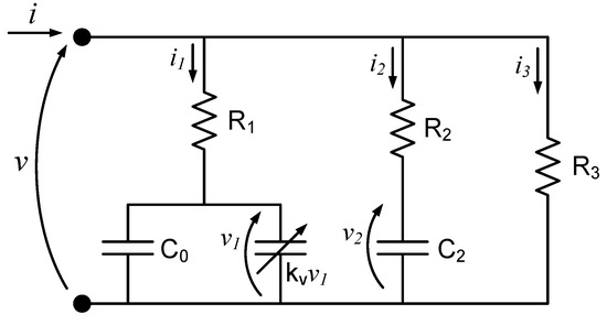
Figure 1.
Two-branch model of DLC.
The two-branch model is well known since it can accurately characterize the DLS behavior during frequent charging-discharging cycles, which is best suited for EV applications where this behavior is exhibited [20].
The first branch consists of three components and models the voltage dependency of the capacitance. This branch gives the DLC a time constant in the order of seconds. The second branch of the equivalent circuit consists of a resistance in series with a capacitance and models the charge redistribution with a time constant of minutes. The third branch consists of one resistor and models the time varying self-discharge, which is modeled as a function of the SC terminal voltage.
The state equations of this circuit are:
where: (n = 0, 2, 3), and (see [9] for the justification of this formula).
2.2. Analysis of the 2-Branch Model
From Figure 1, the two-branch model is analyzed using conventional circuit analysis techniques. By following [9], the assumption R1 = 0 is made, which is reasonable for a DLC [9,15]. Moreover, R3 is assumed known, since this parameter, which is the leakage resistance, is not difficult to find experimentally by using a discharge test without any external load [9]. Moreover, the attempt to retrieve it by using this approach, although theoretically possible, gives rise to an ill-conditioned problem.
Thus, the input current and the voltage output relationships, considering , can be written as:
This equation gives rise to a linear matrix equation, in the same fashion as in [9], as follows:
where is the unknown column vector whose values are:
These parameters present the following nonlinear constraint:
The matrix has the following columns:
and:
The length m of each column corresponds to the number of data points. From Equations (4a)–(4e), the physical parameters can be estimated by using the following formulas, considering that is assumed known:
Noting that and have the same order of magnitude of and that is far smaller than , it follows that cannot be accurately estimated because of the numerical cancellation problem, which implies here a loss of one or two significant digits. This is also valid for . As a consequence, only their product can be correctly estimated. Indeed, this is equal to . For this reason, only , , and will be estimated.
It must be remarked that in order to retrieve all of the parameters, the matrix A must be full-rank and the persistent excitation theorem must be satisfied. Indeed, if a constant current were given, then the matrix becomes rank-deficient in steady-state, and the information on parameter is lost. Furthermore, under these conditions, the constraint vanishes. In a similar way, any experiment corresponding to a ramp output voltage without transient would result in the second derivative of the voltage being always null and the A matrix would be also rank-deficient and consequently could not be estimated. The general idea is to give enough information in the input signals, so that the A matrix is never rank-deficient. In this paper, unlike [13], the input current will be a ramp, so as to retrieve also .
3. Methodology
3.1. Algorithms Adopted
The parameters have been computed by following the three following steps:
- By using the Ordinary Least Squares (OLS) regression off-line to solve Equation (3), but without using the constraint as expressed in Equations (4a)–(4e). This has been performed in simulation and experimentally and has been used as starting point for the subsequent minimization,
- By considering the following minimization problem:which has been solved by using the interior point method. This has been performed in simulation as well as experimentally. The initial values of this constrained minimization (CMM) routine are set by the results of OLS.
- By using the Faranda method which is conducted off-line and specific to two-branch models of SC on experimental data for comparison [15].
The algorithms adopted in 1 and 2 above, are linked and represented in Figure 2.
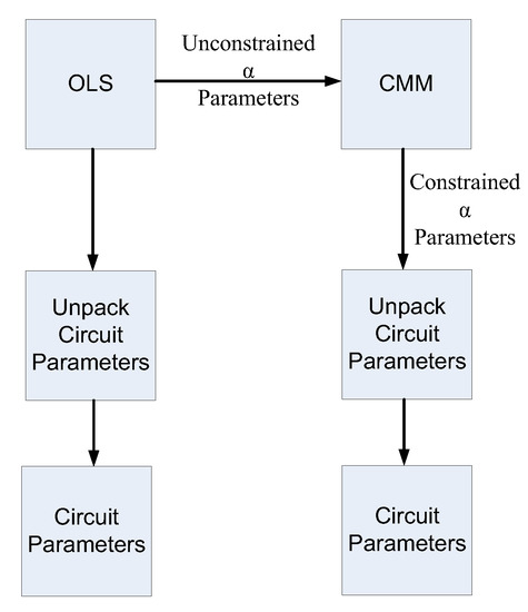
Figure 2.
Algorithms adopted for the purpose of this research work.
3.2. Signal Processing System
In order to process on-line the voltage and currents a suitable signal processing system must be devised as explained in [13]. The scheme in Figure 3 shows the flow of the data and its interconnection with the parameter estimation algorithm.
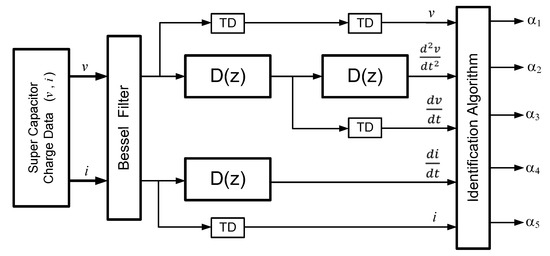
Figure 3.
Block diagram of the signal processing system.
The SC Charging Current and Voltage data is first processed with an anti-aliasing Bessel filter, chosen for its linear phase, and then taken through two identical FIR Derivative Filters, , to compute the first derivative of the current and voltage required by the columns of the matrix A (Figure 3). Whilst the main purpose of the filter is to take the derivative of the data; it is important to point out that is in itself a low-pass filter which helps to remove any high frequency noise that can affect the subsequent stages in the scheme. Another filter is also added to compute the second derivative of the voltage. Since all the filters are FIR ones with linear phase, it is easy to compute the time delays TD by which the signals should be shifted in time so that all columns of A are synchronized.
MATLAB® has been used to design a 50th order FIR tuned to have a passband frequency of 100 Hz and stop band frequency at 180 Hz. The magnitude frequency response and the phase response of the filter is shown in Figure 4. The group delay of the Digital Derivative Filter is determined to be 25 samples from the Group Delay plot as shown in Figure 5. The sampling frequency adopted is fs = 1 kHz.
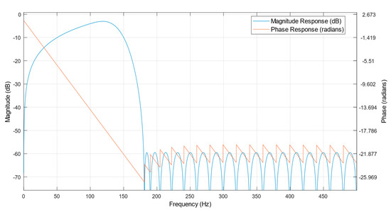
Figure 4.
The magnitude and phase frequency response of the Digital Derivative Filter .
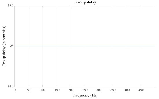
Figure 5.
The Group Delay of the Digital Derivative Filter .
4. Simulation
Simulation Results with a Ramp Input Current
The Faranda method [15] was applied to the experimental charge and self-discharge curves in order to estimate the parameters for the two-branch model. The simulations have been made by using the following set of parameters which have been identified as stated earlier for the circuit of Figure 1 and assuming known and equal to 50 kΩ. The parameters used for the simulation as derived by using the Faranda method are given in Table 1. In this research, all processing, simulation data as well as experimental data were performed in the MATLAB®-Simulink® environment running on a PC with an Intel i5 processor.

Table 1.
Parameters of the DLC.
As explained earlier, a constant current test would not be advisable because of the presence of the column in the A matrix, which would make the matrix rank-deficient. For this reason, a ramp input has been applied. Figure 6 depicts the input current, while Figure 7 depicts the corresponding voltage output.
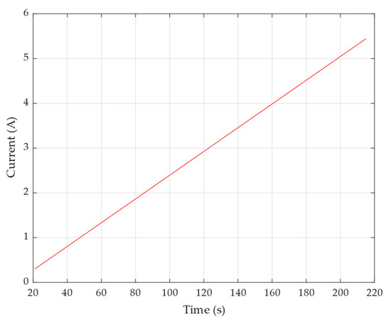
Figure 6.
Input ramp current.
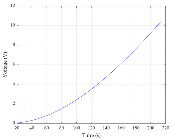
Figure 7.
Output voltage.
For the retrieval of the parameters two methods have been applied, as explained in Section 3.1: (1) the OLS method, which gives an unconstrained solution, and then (2) a constrained minimization algorithm (interior point method) as shown in Figure 2. through to have been generated using the family of equations listed in Equations (4a)–(4e), and for the purpose of software validation discussed in this section, these values are considered as “true” and listed in Table 2.
Table 2.
Alpha Parameters Estimation Results by OLS with an Input Ramp Current (Simulation).
Table 2 indicates that the results obtained using the OLS method for the alpha parameters are unsatisfactory, with errors ranging from approximately 2% to as much as 44%. Only can be estimated with a reasonable degree of accuracy.
By using Equations (8a)–(8c), the physical parameters, as summarized in Table 3, only two parameters have been retrieved acceptably.
Table 3.
DLC Parameter Estimation Results by OLS with a Ramp Current as Input (Simulation).
The above results show the need to use the constraint Equation (5). The results obtained after applying an input ramp current to Constrained Minimization Method (CMM) appear very good, as shown in Table 4 for the alpha parameters: errors remain generally below 11%. The OLS estimator did not perform to a desired standard due to the fact that OLS method is simplistic and was blind to the non-linear constraint in Equation (5). This resulted in the circuit parameters being unpacked from the unconstrained parameters resulting in undesirable errors. However, CMM has a much better result as it respects the non-linear constraint mentioned above. The constraint has the effect that if it is respected, the search space for the CMM is greatly reduced, allowing for faster convergence. It was also noted that when the constraint is respected, parameter estimation is much more accurate.
Table 4.
Alpha Parameter Estimation Results by CMM with an Input Ramp Current (Simulation).
The physical parameters, obtained with the alpha parameters by using Equations (8a)–(8c), have percentage errors lower than 9%. The results are summarized in Table 5.
Table 5.
DLC Parameter Estimation Results by CMM with a Ramp Current as Input (Simulation).
Finally, Figure 8 shows the error of the cost function as well as its fast convergence to zero just within 26 iterations by using CMM. These 26 iterations take a total of 15 s.
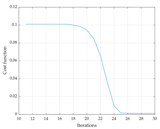
Figure 8.
Cost function of CMM for Alpha Parameter Estimation in Simulation.
5. Experimental Verifications
5.1. The Super Capacitor Bank
Figure 9 shows the experimental rig which is composed of a “Green-Cap” MH47765 Super Capacitor bank of 6 × DLSC connected in series. Each single DLSC cell is 500 F with a voltage rating of 2.7 V.
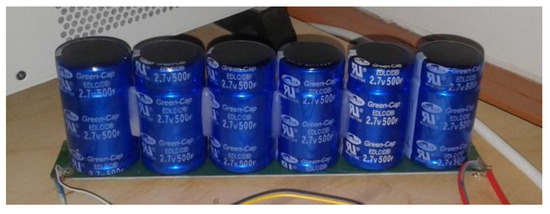
Figure 9.
The 88.33 F SC bank used for the experiments.
The series configuration results in the net capacitance of the Bank, CBank, becoming 83.33 F. The voltage rating of the SC Bank is calculated to be 16.2 V. A 10 Ω load resistor has been used in the discharge circuit only which results in a time constant, , of 833 s.
Some of the other important parameters of the SC Bank from the data sheet [43] are presented here:
- ESR @ 1 kHz = 18 mΩ
- ESR in DC = 30 mΩ
- Max. Peak Current = 20 A
- Max. Continuous Current = 167 A
- Rated Voltage = 15 V
5.2. Experimental Rig
The SC is placed in a dual charge/discharge circuit where a two-way switch is used to change the SC connection from the charging system to the discharging system as shown in Figure 10. In both of these cases, the Data Acquisition System remains connected to the terminals of the CBank.
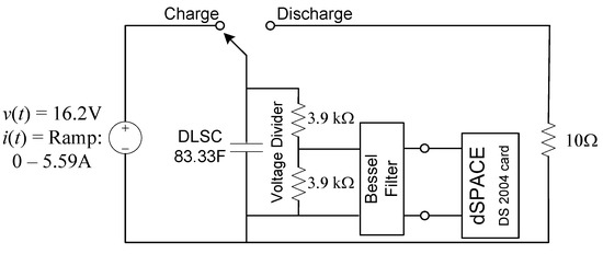
Figure 10.
The experimental charge/discharge circuit connected to the data acquisition system.
The Data Acquisition System consists of the dSPACE AutoBox DS1007 System. The DS2004 card has been used, which is the dSPACE card used to read an Input Analog Signal. The input range of the DS2004 card is 0–10 V. Since the full charge of the CBank is 16.2 V, a voltage divider has been used as an intermediary to the dSPACE system. A National Instruments (NI) USB 6211 DAQ system was utilized as a redundant data capture system but did not play any crucial role as dSPACE delivered better results. The sampling frequency of 1 kHz has been selected for the charge and discharge tests. The Experimental Test Rig is shown in Figure 11.
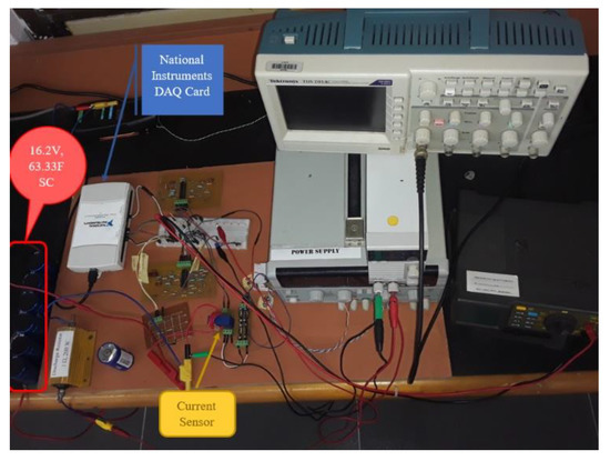
Figure 11.
Experimental setup showing SC Bank.
5.3. Experimental Determination of R3
In order to experimentally determine the value of Leakage Resistance or Effective Parallel Resistance, R3, a basic approach has been applied [44]. The RC time constant is given by: .
In this experiment, the SC is first fully charged to 16.2 V and then a Digital Multimeter (DMM) is used to check the voltage of the SC every 12 h. Such a large sampling time has been selected due to the long self-discharge time which is in the order of weeks. Furthermore, note the deliberate choice of using a DMM in the design of this experiment in contrast to using a normal DAQ system due to the fact that any internal impedance present in the DAQ system could load the SC and affect the time constant. The DMM is not continually connected to the SC but only momentarily during the designated voltage recording times.
The SC is allowed to self-discharge with zero loading condition to a value of 36.8% of 16.2 V which computes to 5.96 V. The selected percentage value is computed from the reciprocal of the Euler’s number, e. Further treatment of this can be found in [44]. After executing the experiment in this section, the time taken for this self-discharge of the SC to the stated level is 51.5 days or 4,449,600 s, resulting in having a value of .
5.4. The Bessel Filter
As discussed in Section 3.2, the proposed Signal Processing Scheme consists of analog Anti-Aliasing Filter realized in hardware. The purpose of this filter is to remove anti High Frequency noise which may affect the subsequent stages. A Fourth-Order Low-Pass Bessel Filter has been selected to be the Anti-Aliasing filter in this case due to its linear phase. In order to achieve this, the MAX274ACNG chip manufactured by MAXIM is utilized as per instructions in its datasheet [45]. The cut-off frequency is set at a low 40 Hz.
The MAX274 chip consists of continuous-time active filters consisting of four second order sections. Each section is then implemented into a low-pass filter response and is programmed by four external resistors. Using the standard resistor values and parallel and/or series connections, the exact values for the resistors have been obtained.
5.5. The Ramp Current Generator
An integral part of the proposed scheme is to charge the SC with a constant Ramp Current. This constant Ramp Current is generated by means of a Regulated DC power supply with a variable current limiter. In this experiment, a TEXIO Brand, Model # PS 60-6, Regulated DC Power Supply is utilized. This TEXIO Power Supply consists of a regulated variable DC voltage supply up to a limit of 50 V and with current limited up to 6 A.
Since the SC has a voltage rating of 16.2 V, the voltage supply is pre-set to the same. The Current Limit is initially set at 0 A. The variable Current Limit Controller is utilized to achieve a constant Ramp Current by gradually increasing the limit gradient so as to achieve a constant ramp. This results in a Linear Current Ramp as clearly depicted in Figure 12 which shows a Linear Ramp starting from 0 A and rising linearly to 5.59 A over a period of 34,000 ms.
5.6. Experimental Charge Curves
The graphs in Figure 12 and Figure 13 show only the charging curves of the CBank with an input step current and an input ramp current, respectively. The step current has a constant value of 6 A. For the input ramp current, the ramp starts at 0 A and rises with constant slope to a value of 5.6 A. Notice that for both Figure 12 and Figure 13, the current rolls down exponentially once the CBank if fully charged. These are the values adopted for the experimental verification of the method.

Figure 12.
Experimental Current and Voltage charge curve of a 16.2 V 83.33 F EDLC with a step current of 6 A.

Figure 13.
Experimental Current and Voltage charge curve of a 16.2 V—83.33 F EDLC with a ramp current 0–5.59 A.
6. Results and Discussion for Experimental Data
In the proposed methodology, OLS is applied to compute the parameters of the experimental results shown in Table 6 and Table 7. The results with OLS experimental results method are not acceptable since some parameters are negative, which is meaningless, but the solution will be used as a starting point for the constrained minimization. The parameters obtained are compared with those obtained with the method of Faranda, both in terms of physical parameters and alpha parameters. The reason why Faranda is chosen as a comparator against the proposed method is because Faranda’s method results in parameters for the two-branch model which is the model used to develop the proposed method.
Table 6.
Alpha Parameter Estimation Results by OLS with Experimental Data using an Input Ramp Current and compared against Faranda.
Table 7.
DLC Parameter Estimation Results by OLS with Real Experimental Data and a Ramp Current as Input together with comparison to Faranda.
The Constrained Minimization Method (CMM) is then used to compute the parameters of the DLC with experimental data as shown in Table 8 and Table 9 below. In order to facilitate the solution, some reasonable upper and lower bounds have been given in Table 8. The upper and lower bounds were chosen using the Faranda method and the research work of [46] in conjunction with and through deduction. The upper and lower bounds were chosen using the Faranda method and the research work outlined by [46] in conjunction with and through deduction. For example, a SC cannot have which is any greater than that specified by its manufacturer. The circuit parameters, upper and lower bounds are then extended into the parameters as shown in Table 8.
Table 8.
Alpha Parameter Estimation Results by CMM with Real Experimental Data compared against Faranda.
Table 9.
DLC Parameter Estimation Results by CMM with Real Experimental Data and a Ramp Current as Input together with comparison to Faranda.
Figure 14 shows the cost function vs iterations of the CMM method. In this figure the minimum of the cost function is reached after only 5 iterations which took 6 s.
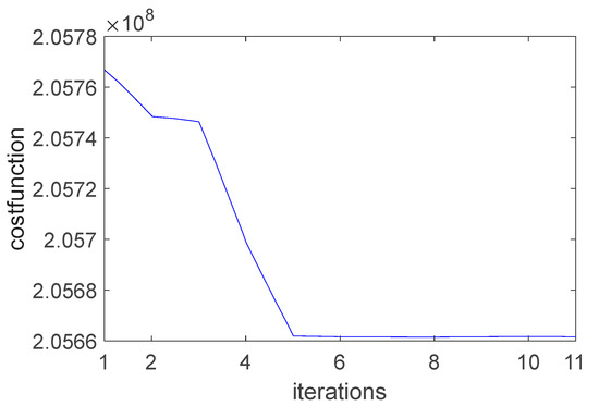
Figure 14.
Cost function of CMM for Alpha Parameter Estimation with Real Experimental Data.
As demonstrated in Figure 15, the voltage curve generated using the CMM-derived parameters outlined in Section 2 more closely approximates the actual experimental curve compared to the curve derived using Faranda’s method. Although the proposed approach yields results that are comparable to Faranda’s, it circumvents the need for the cumbersome and numerous steps involved, thereby resulting in faster computation of the circuit parameters. However, the true advantage of the proposed method lies in its nearly instantaneous processing time.

Figure 15.
Output voltage comparison between the CMM and the Faranda parameters.
While the proposed method offers several advantages, it is worth noting that it has one notable limitation: if the experimental voltage and current inputs to the perimeter engine are noisy, the signal processing scheme’s first and second derivative stages may amplify the noise and lead to unrealistic outputs. However, this issue is not unique to the proposed method, as noise can impact the accuracy of many estimation techniques. Therefore, the proposed method still presents a promising and efficient solution for parameter estimation in the absence of significant noise in the experimental data.
7. Conclusions
This paper has proposed a refined approach to retrieving the parameters of a DLC, which addresses the limitations of the OLS method by utilizing a CMM. The CMM imposes a constraint in the state equations, which allows for more accurate parameter estimation than the unconstrained OLS method. The proposed method has been evaluated using both simulation and experimental data and has been shown to provide more accurate and reliable results than the OLS method. One of the main advantages of the proposed method is its simplicity and efficiency. Unlike other existing methods, the proposed CMM approach requires only an input current ramp and the corresponding output voltage, as well as suitable signal-processing conditioning to compute the derivatives. This significantly reduces the number of laborious steps required to obtain accurate parameter estimates, resulting in faster computation of circuit parameters. However, the retrieval of the leakage resistance parameter remains a challenging task due to numerical ill-conditioning. To overcome this limitation, the authors suggest an alternative approach to estimating the leakage resistance parameter, which involves a simple discharge experiment of the supercapacitor without load. This approach allows for more accurate and reliable estimation of the leakage resistance parameter, which is crucial for accurate parameter retrieval. The proposed strategy has been compared to the method of Faranda, which is a widely used method for parameter retrieval in DLCs and show a relative error of close to 5% for two of the three parameters. The results show that the proposed CMM approach provides comparable results to the Faranda method while being more efficient and requiring fewer steps. The almost instantaneous processing time of the proposed method is also a significant advantage over the conventional methods, making it a promising solution for practical applications such as for SCs which are utilized in EVs where the SC parameters may be used for diagnostics and finding the SOH.
Author Contributions
All authors contributed equally to the conceptualization of this research. The methodology was developed by N.I.J., G.C. and M.C., while R.R.K. and G.C. carried out the validation and formal analysis. Investigation was performed by N.I.J., R.R.K. and A.M., and resources were provided by G.C. and M.C.; N.I.J. curated the data, and the original draft of the manuscript was prepared by N.I.J. All authors contributed to writing, review, and editing of the manuscript. Visualization was performed by N.I.J., while supervision was provided by G.C. and M.C. Project administration was handled by R.R.K. and G.C., and funding was acquired by M.C. All authors have read and agreed to the published version of the manuscript.
Funding
This research was funded by the School of Information Technology, Engineering, Mathematics and Physics (STEMP) Research Committee. The APC was funded by the office of the Head of School of STEMP, USP.
Data Availability Statement
The data can be shared up on request.
Conflicts of Interest
The authors declare no conflict of interest.
References
- Ehsani, M.; Gao, Y.; Emadi, A. Fundamentals, Theory, and Design, 2nd ed.; CRC Press: Boca Raton, FL, USA, 2017; ISBN 978-1-315-21940-0. [Google Scholar]
- Dey, S.; Mohon, S.; Pisu, P.; Ayalew, B.; Onori, S. Online State and Parameter Estimation of Battery-Double Layer Capacitor Hybrid Energy Storage System. In Proceedings of the 2015 54th IEEE Conference on Decision and Control (CDC), Osaka, Japan, 15–18 December 2015; pp. 676–681. [Google Scholar]
- Cao, J.; Emadi, A. A New Battery/UltraCapacitor Hybrid Energy Storage System for Electric, Hybrid, and Plug-In Hybrid Electric Vehicles. IEEE Trans. Power Electron. 2012, 27, 122–132. [Google Scholar] [CrossRef]
- Devillers, N.; Jemei, S.; Péra, M.-C.; Bienaimé, D.; Gustin, F. Review of Characterization Methods for Supercapacitor Modelling. J. Power Sources 2014, 246, 596–608. [Google Scholar] [CrossRef]
- Farhadi, M.; Mohammed, O. Energy Storage Technologies for High-Power Applications. IEEE Trans. Ind. Appl. 2016, 52, 1953–1961. [Google Scholar] [CrossRef]
- Shen, X.; Chen, S.; Li, G.; Zhang, Y.; Jiang, X.; Lie, T.T. Configure Methodology of Onboard Supercapacitor Array for Recycling Regenerative Braking Energy of URT Vehicles. IEEE Trans. Ind. Appl. 2013, 49, 1678–1686. [Google Scholar] [CrossRef]
- Rafik, F.; Gualous, H.; Gallay, R.; Crausaz, A.; Berthon, A. Frequency, Thermal and Voltage Supercapacitor Characterization and Modeling. J. Power Sources 2007, 165, 928–934. [Google Scholar] [CrossRef]
- Zubieta, L.; Bonert, R. Characterization of Double-Layer Capacitors for Power Electronics Applications. IEEE Trans. Ind. Appl. 2000, 36, 199–205. [Google Scholar] [CrossRef]
- Pucci, M.; Vitale, G.; Cirrincione, G.; Cirrincione, M. Parameter Identification of a Double-Layer-Capacitor 2-Branch Model by a Least-Squares Method. In Proceedings of the IECON 2013—39th Annual Conference of the IEEE Industrial Electronics Society, Vienna, Austria, 10–13 November 2013; pp. 6770–6776. [Google Scholar]
- Kitahara, A.; Watanabe, A. (Eds.) Electrical Phenomena at Interfaces (Fundamentals, Measurements and Applications); Marcel Dekker: New York, NY, USA, 1984. [Google Scholar]
- Morrison, S.R. The Chemical Physics of Surfaces; Springer Science & Business Media: Berlin, Germany, 2013; ISBN 978-1-4899-2498-8. [Google Scholar]
- Maundy, B.J.; Elwakil, A.; Freeborn, T.; Allagui, A. Improved Method to Determine Supercapacitor Metrics from Highpass Filter Response. In Proceedings of the 2016 28th International Conference on Microelectronics (ICM), Giza, Egypt, 17–20 December 2016; pp. 25–28. [Google Scholar]
- Buller, S.; Karden, E.; Kok, D.; De Doncker, R.W. Modeling the Dynamic Behavior of Supercapacitors Using Impedance Spectroscopy. IEEE Trans. Ind. Appl. 2002, 38, 1622–1626. [Google Scholar] [CrossRef]
- Halper, M.S. Supercapacitors: A Brief Overview; MITRE: McLean, VA, USA, 2006; pp. 1–41. [Google Scholar]
- Faranda, R. A New Parameters Identification Procedure for Simplified Double Layer Capacitor Two-Branch Model. Electr. Power Syst. Res. 2010, 80, 363–371. [Google Scholar] [CrossRef]
- Sakka, M.A.; Gualous, H.; Omar, N.; Mierlo, J.V.; Sakka, M.A.; Gualous, H.; Omar, N.; Mierlo, J.V. Batteries and Supercapacitors for Electric Vehicles; IntechOpen: London, UK, 2012; ISBN 978-953-51-0893-1. [Google Scholar]
- IEC 62576:2018|IEC Webstore. Available online: https://webstore.iec.ch/publication/28801 (accessed on 23 January 2023).
- Logerais, P.O.; Camara, M.A.; Riou, O.; Djellad, A.; Omeiri, A.; Delaleux, F.; Durastanti, J.F. Modeling of a Supercapacitor with a Multibranch Circuit. Int. J. Hydrogen Energy 2015, 40, 13725–13736. [Google Scholar] [CrossRef]
- Drummond, R.; Howey, D.A.; Duncan, S.R. Parameter Estimation of an Electrochemical Supercapacitor Model. In Proceedings of the 2016 European Control Conference (ECC), Aalborg, Denmark, 29 June–1 July 2016; IEEE: Piscataway, MJ, USA, 2016; pp. 1–6. [Google Scholar]
- Reichbach, N.; Kuperman, A. Recursive-Least-Squares-Based Real-Time Estimation of Supercapacitor Parameters. IEEE Trans. Energy Convers. 2016, 31, 810–812. [Google Scholar] [CrossRef]
- Eddahech, A.; Ayadi, M.; Briat, O.; Vinassa, J.-M. Online Parameter Identification for Real-Time Supercapacitor Performance Estimation in Automotive Applications. Int. J. Electr. Power Energy Syst. 2013, 51, 162–167. [Google Scholar] [CrossRef]
- Freeborn, T.J.; Maundy, B.; Elwakil, A.S. Measurement of Supercapacitor Fractional-Order Model Parameters From Voltage-Excited Step Response. IEEE J. Emerg. Sel. Top. Circuits Syst. 2013, 3, 367–376. [Google Scholar] [CrossRef]
- Oukaour, A.; Pouliquen, M.; Tala-Ighil, B.; Gualous, H.; Pigeon, E.; Gehan, O.; Boudart, B. Supercapacitors Aging Diagnosis Using Least Square Algorithm. Microelectron. Reliab. 2013, 53, 1638–1642. [Google Scholar] [CrossRef]
- Vitale, G. Supercapacitor Modelling by Lagrange’s Equations; EEEJ: Las Palmas de Gran Canaria, Spain, 2016; Volume 1, pp. 127–132. [Google Scholar]
- Alonge, F.; Rodonò, G.; Cirrincione, M.; Vitale, G. Supercapacitor Diagnosis Using an Extended Kalman Filtering Approach. In Proceedings of the 2016 IEEE 16th International Conference on Environment and Electrical Engineering (EEEIC), Florence, Italy, 7–10 June 2016; pp. 1–6. [Google Scholar]
- Nadeau, A.; Sharma, G.; Soyata, T. State-of-Charge Estimation for Supercapacitors: A Kalman Filtering Formulation. In Proceedings of the 2014 IEEE International Conference on Acoustics, Speech and Signal Processing (ICASSP), Florence, Italy, 4–9 May 2014; pp. 2194–2198. [Google Scholar]
- Zhang, L.; Wang, Z.; Sun, F.; Dorrell, D.G. Online Parameter Identification of Ultracapacitor Models Using the Extended Kalman Filter. Energies 2014, 7, 3204–3217. [Google Scholar] [CrossRef]
- Nonlinear Extension of Battery Constrained Predictive Charging Control with Transmission of Jacobian Matrix|Elsevier Enhanced Reader. Available online: https://reader.elsevier.com/reader/sd/pii/S014206152200758X?token=D6E214EE9322B88D938DA48FE1FC341540098929F043EA1C45991DAE9C0EEA8BCBD06100680774AED9CE8425C8AB38C6&originRegion=us-east-1&originCreation=20230426011722 (accessed on 26 April 2023).
- Saha, P.; Dey, S.; Khanra, M. Modeling and State-of-Charge Estimation of Supercapacitor Considering Leakage Effect. IEEE Trans. Ind. Electron. 2020, 67, 350–357. [Google Scholar] [CrossRef]
- Naseri, F.; Farjah, E.; Ghanbari, T.; Kazemi, Z.; Schaltz, E.; Schanen, J.-L. Online Parameter Estimation for Supercapacitor State-of-Energy and State-of-Health Determination in Vehicular Applications. IEEE Trans. Ind. Electron. 2020, 67, 7963–7972. [Google Scholar] [CrossRef]
- El Mejdoubi, A.; Chaoui, H.; Gualous, H.; Sabor, J. Online Parameter Identification for Supercapacitor State-of-Health Diagnosis for Vehicular Applications. IEEE Trans. Power Electron. 2017, 32, 9355–9363. [Google Scholar] [CrossRef]
- Shi, Z.; Auger, F.; Schaeffer, E.; Guillemet, P.; Loron, L. Interconnected Observers for Online Supercapacitor Ageing Monitoring. In Proceedings of the IECON 2013—39th Annual Conference of the IEEE Industrial Electronics Society, Vienna, Austria, 10–13 2013; IEEE: Piscataway, MJ, USA, 2013; pp. 6746–6751. [Google Scholar]
- Chaoui, H.; El Mejdoubi, A.; Oukaour, A.; Gualous, H. Online System Identification for Lifetime Diagnostic of Supercapacitors With Guaranteed Stability. IEEE Trans. Control Syst. Technol. 2016, 24, 2094–2102. [Google Scholar] [CrossRef]
- Dănilă, E.; Livint, G.; Lucache, D.D. Dynamic Modelling of Supercapacitor Using Artificial Neural Network Technique. In Proceedings of the 2014 International Conference and Exposition on Electrical and Power Engineering (EPE), Iasi, Romania, 16–18 October 2014; pp. 642–645. [Google Scholar]
- Marie-Francoise, J.-N.; Gualous, H.; Berthon, A. Supercapacitor Thermal- and Electrical-Behaviour Modelling Using ANN. IEE Proc.-Electr. Power Appl. 2006, 153, 255–262. [Google Scholar] [CrossRef]
- Eddahech, A.; Briat, O.; Ayadi, M.; Vinassa, J.-M. Modeling and Adaptive Control for Supercapacitor in Automotive Applications Based on Artificial Neural Networks. Electr. Power Syst. Res. 2014, 106, 134–141. [Google Scholar] [CrossRef]
- Farsi, H.; Gobal, F. Artificial Neural Network Simulator for Supercapacitor Performance Prediction. Comput. Mater. Sci. 2007, 39, 678–683. [Google Scholar] [CrossRef]
- Miniguano, H.; Barrado, A.; Fernández, C.; Zumel, P.; Lázaro, A. A General Parameter Identification Procedure Used for the Comparative Study of Supercapacitors Models. Energies 2019, 12, 1776. [Google Scholar] [CrossRef]
- Fathy, A.; Rezk, H. Robust Electrical Parameter Extraction Methodology Based on Interior Search Optimization Algorithm Applied to Supercapacitor. ISA Trans. 2020, 105, 86–97. [Google Scholar] [CrossRef] [PubMed]
- Jannif, N.I.; Ram, K.; Bangalini, K.; Loli, A.; Mohammadi, A.; Cirrincione, M. Supercapacitor Parameter Estimation and Hybridyzation with PEMFC for Purge Compensation. In Proceedings of the 2022 International Symposium on Power Electronics, Electrical Drives, Automation and Motion (SPEEDAM), Sorrento, Italy, 22–24 June 2022; pp. 70–75. [Google Scholar]
- Prasad, R.; Mehta, U.; Kothari, K.; Cirrincione, M.; Mohammadi, A. Supercapacitor Parameter Identification Using Grey Wolf Optimization and Its Comparison to Conventional Trust Region Reflection Optimization. In Proceedings of the 2019 International Aegean Conference on Electrical Machines and Power Electronics (ACEMP) & 2019 International Conference on Optimization of Electrical and Electronic Equipment (OPTIM), Istanbul, Turkey, 27–29 August 2019; pp. 563–569. [Google Scholar]
- Jannif, N.I.; Cirrincione, G.; Cirrincione, M.; Mohammadi, A.; Vitale, G. Experimental Application of Least-Squares Technique for Estimation of Double Layer Super Capacitor Parameters. In Proceedings of the 2017 20th International Conference on Electrical Machines and Systems (ICEMS), Sydney, Australia, 11–14 August 2017; pp. 1–5. [Google Scholar]
- Samwha Datasheet & Applicatoin Notes—Datasheet Archive. Available online: https://www.datasheetarchive.com/Samwha-datasheet.html (accessed on 24 January 2023).
- Alexander, C.K.; Sadiku, M.N.O. Fundamentals of Electric Circuits; McGraw-hill Education: New York, NY, USA, 2017; ISBN 978-1-259-25132-0. [Google Scholar]
- Max275 Datasheet—4th- and 8th-Order, Continuous-Time Active Filters. Available online: https://www.digchip.com/datasheets/parts/datasheet/280/MAX275.php (accessed on 24 January 2023).
- Solano, J.; Hissel, D.; Pera, M.-C. Modeling and Parameter Identification of Ultracapacitors for Hybrid Electrical Vehicles. In Proceedings of the 2013 IEEE Vehicle Power and Propulsion Conference (VPPC), Beijing, China, 15–18 October 2013; IEEE: Piscataway, MJ, USA, 2013; pp. 1–4. [Google Scholar]
Disclaimer/Publisher’s Note: The statements, opinions and data contained in all publications are solely those of the individual author(s) and contributor(s) and not of MDPI and/or the editor(s). MDPI and/or the editor(s) disclaim responsibility for any injury to people or property resulting from any ideas, methods, instructions or products referred to in the content. |
© 2023 by the authors. Licensee MDPI, Basel, Switzerland. This article is an open access article distributed under the terms and conditions of the Creative Commons Attribution (CC BY) license (https://creativecommons.org/licenses/by/4.0/).