Article

Short-Term Power Load Forecasting Based on Feature Filtering and Error Compensation under Imbalanced Samples

College of Automation Engineering, Shanghai University of Electric Power, Shanghai 200090, China
*
Author to whom correspondence should be addressed.
Energies 2023, 16(10), 4130; https://doi.org/10.3390/en16104130
Submission received: 5 May 2023 / Revised: 10 May 2023 / Accepted: 15 May 2023 / Published: 16 May 2023
(This article belongs to the Section F: Electrical Engineering)

Abstract

:
There are many influencing factors present in different situations of power load. There is also a strong imbalance in the number of load samples. In addition to examining the problem of low training efficiency of existing algorithms, this paper proposes a short-term power load prediction method based on feature selection and error compensation under imbalanced samples. After clustering the load data, we expand some sample data to balance the sample categories and input the load data and filtered feature sequences into the improved GRU for prediction. At the same time, the errors generated during the training process are used as training data. An error correction model is constructed and trained, and the results are used for error compensation to further improve prediction accuracy. The experimental results show that the overall prediction accuracy of the model has increased by 80.24%. After expanding a few samples, the prediction accuracy of the region where the samples are located increased by 59.41%. Meanwhile, due to the improvement of the algorithms, the running time was reduced by approximately 14.92%.

1. Introduction

Electricity load forecasting is important for grid planning as well as smooth and safe grid operation [1,2]. The common short-term electric load is usually forecasted in hours or minutes as the basic unit [3,4]. Scholars at home and abroad have carried out extensive and in-depth research on the theory and related methods of load forecasting [5,6].
Compared to other types of time-series data, electricity loads are more random and volatile and are influenced by many factors [7,8], such as weather conditions, geographical location, holidays, and time-of-day tariffs, which can all interfere with electricity consumption [9]. By introducing feature quantities to the forecasting model and training the features and load together, the fit of the data to the model can be improved to a certain extent, thus enabling the forecasting model to gain stronger predictive power [10]. The methods in the literature [11] do not filter the feature quantity of the electricity, so a larger number of features will be input to the prediction model, which not only affects the training but also inevitably has an impact on the model’s stability. The above problem can be effectively improved by filtering the number of input feature terms. In the existing literature, most of the input feature sequence characteristics are extracted directly using algorithms. If the feature sequence is decomposed to enhance regularity, the extraction of data features can be effectively improved. Traditional data decomposition methods have difficulty in dealing with signals with features such as non-linearity and irregularity, so the empirical mode decomposition (EMD) algorithm, which overcomes the above problems, is widely used [12,13,14]. One study [15] used EMD to decompose the load data, and due to the recursive nature of the EMD algorithm itself, the problem of over-decomposition occurred, with the data being decomposed into more components and the computational effort increasing significantly. Therefore, another study [16] proposed the variational mode decomposition (VMD) algorithm, which is an adaptive approach to signal decomposition that can effectively solve the problems that exist in EMD and its improved algorithms [17,18]. One study [19] applied VMD, and not only did the decomposed sequences show a strong regularity, but the number of subsequences decomposed by VMD was also substantially reduced compared to the EMD decomposition. However, the problem is also revealed that the VMD requires the setting of operational parameters, which, if not properly set, may not result in the decomposed sequences being characterized. Therefore, using the whale optimization algorithm (WOA) to optimize the parameters of the VMD can effectively improve the value of the VMD and save the extra time consumed by the parameter adjustment.
With the continuous development of neural-network-like algorithms, there have been successive applications of neural network algorithms such as recurrent neural network (RNN), long-short-term-memory (LSTM) neural network [20,21], and gated recurrent unit (GRU) for power load forecasting [22,23]. One study [24] used LSTM as the main prediction model, due to the inherent characteristics of LSTM and the large number of input data features, which made the training time longer. Another study [25] used GRU as the main algorithm for prediction. GRU is an improved algorithm of LSTM. Compared with LSTM, GRU has improved prediction accuracy. At the same time, the training efficiency has been improved. Another study [26] combined the improved VMD and GRU algorithms to make predictions by decomposing the original data and then predicting, with a large improvement in the results compared to existing models. These papers also reflect the fact that neural network algorithms such as LSTM and GRU have the problem of slow training speed in the case of multiple feature inputs. In this paper, the traditional GRU is decomposed, and an intermediate shared layer is added to effectively improve the training speed while maintaining accuracy.
A practical problem that tends to be overlooked in existing studies is the imbalance that occurs in the electricity load data sample. In actual data samples, there is a significant difference in the electricity consumption characteristics between weekday and holiday electricity loads, and the sample size for holidays shows a significant imbalance compared to that of weekdays. In the literature [27], the accuracy of load forecasting is low for an unbalanced minority of samples, such as holidays, when compared to weekdays. Such phenomena occur because the proportion of holiday data samples to the total sample is too low. Due to the small sample size, it is difficult for the model to learn the characteristics of the minority samples, and this deficiency will cause the problem of low accuracy of electricity load forecasting on holidays, resulting in a reduction of the total forecasting accuracy, and therefore the problem of unbalanced electricity load data needs to be addressed. A synthetic minority based on probabilistic distribution (SyMProD) was proposed in the literature [28], which can be expanded to solve the sample imbalance problem for a relatively small percentage of data.
In summary, this paper proposes a new solution: after the features are filtered using kernel principal component analysis (KPCA), they are decomposed into modal components to mine for regularity, and then their temporal features are extracted using a time convolution network. The samples are clustered using K-means and then expanded using the SyMProD method for the smaller samples. Finally, predictions are made using an improved GRU, and an error correction model is constructed for training, using its results for compensation.
The main contributions of the methods proposed in the paper are as follows:
  • Constructing an error compensation model and using the prediction results of the errors to compensate for the original results can effectively improve the overall prediction accuracy.
  • By expanding the minority sample data, the imbalance of the load data is alleviated, and the accuracy of the prediction results in the minority sample area can be effectively improved.
  • Improvements to GRU ensure prediction accuracy while simplifying the model’s structure and improving the overall operational efficiency.
The organizational structure of this article is as follows: Section 2 introduces the data processing process; Section 3 introduces the modeling and improvement of the main algorithms; Section 4 analyzes and discusses the calculation examples; Section 5 provides the conclusion.

2. Data Processing Methods

2.1. Feature Selection Process Based on Kernel Principal Component Analysis

In actual forecasting, electricity load often shows a strong correlation with weather indicators such as temperature and humidity, while other indicators also have an impact, but the correlation does not seem obvious. If all features are directly input into the model for training, it not only affects the training efficiency, but also inevitably has an impact on the stability of the model. Therefore, this paper uses kernel principal component analysis (KPCA) to calculate the contribution rate of input features to remove redundant feature terms [29,30]. The main process of KPCA is as follows:
  • Standardization of data. Find the kernel matrix K and use the radial basis kernel function to complete the mapping of the original data from data space to feature space.
  • The centralized kernel matrix K c is used to correct the kernel matrix K c = K l N K K l N + l N K l N , where l N is the matrix of N × N with 1/N for each element.
  • Calculate the eigenvalues of the matrix K c The eigenvalues determine the magnitude of the variance. Arrange the eigenvalues in descending order to obtain the arranged eigenvector λ 1 , λ 2 , , λ n .
  • Schmitt orthogonalization and unitization of the eigenvectors to obtain the master sequence α 1 , α 2 , , α n
  • Calculate the contribution of each feature value β 1 , β 2 , , β n , and select the first t principal components α 1 , α 2 , , α t as the retained features if β t > p, according to the set requirement p.

2.2. Sample Expansion Methods Based on the Synthesis of a Small Number of Probability Distributions

Synthetic minority based on probabilistic distribution (SyMProD) is a method proposed by the literature [28] to perform sample expansion, which aims to solve the problem of unbalanced sample size in the training sample. The main steps of this method are as follows:
1.
Conducting sample screening
The samples synthesized from the noisy samples will have an impact on the predictive stability of the model, so the noisy samples need to be removed. The outlier data is first removed before sample selection, and the original samples are normalized after the outlier data is removed. Samples with absolute values below a threshold after normalization are the noisy samples removed. Add the denoised samples to the sample set.
2.
Select a few samples and synthesize
After selecting a small number of samples in the sample set, a closeness factor is defined for the selected samples, which is used to determine the degree of overlap between samples. Select x samples that meet the overlap, collect them into S = { S 1 , S 2 , , S x , S x + 1 } , calculate the probability distribution of each sample P, and synthesize the new samples using the following formula X new .
X new = i = 1 x + 1 β i P i S i
In Equation (1), β i is a random value in (0,1); P i is the probability distribution of the ith sample; and S i is the ith sample. In the text, because of the need to ensure the authenticity and diversity of the samples, sample synthesis can only be performed once (i.e., the synthesized samples cannot be used to synthesize again).

3. Modelling and Improvement of Main Algorithm

3.1. Error Compensation Model

In short-term power load forecasting, error compensation is used to improve the prediction accuracy by generating compensation data to offset the errors in the original prediction results, based on the existing features and influencing factors, after secondary training of the errors generated during the training process [31]. For a complete set of models that have been trained, the internal structure, network model, and weighting of each feature are already fixed, and the logical relationship between each variable and the final prediction result can usually be determined when the training is completed. Therefore, as long as the model remains fixed, even if the same data and features are repeatedly input, the same prediction results can be obtained as before. The errors generated during the training of the model are also the result of the fixed set of logical operations performed by the model, so the errors are strongly correlated with the input features and data. Therefore, the errors generated during the training process can be put back into the model for training as training data, so that the model can establish a correlation between the errors and the feature data used for load prediction, thus achieving the prediction of errors, as shown in Figure 1.
In summary, the initial data and features are processed to obtain the data and features for training, which are trained and predicted using the model to obtain the prediction results. The error data generated in the training is put back into the training model above for training and prediction, the error prediction results are obtained, and finally the error prediction results are superimposed on the previous prediction results to compensate for them and obtain the final prediction values.

3.2. Optimizing VMD with WOA

The whale optimization algorithm (WOA) is a meta-heuristic algorithm that simulates the hunting behavior of humpback whales [32]. Compared with traditional heuristics, the WOA algorithm is more accurate, converges well, is stable, and is less likely to fall into a local optimum, so WOA is able to find the global optimal solution more consistently.
The core of variational modal decomposition (VMD) is the construction and solution of a variational problem. Unlike the circular elimination approach of EMD and its modifications, VMD uses an iterative process to complete the search for the optimal solution and finally decomposes the signal into K intrinsic mode functions (IMFs), each with a different central frequency band.
The VMD decomposition uses the minimum value of the sum of the IMF center frequencies as the objective function for the construction of the variational problem. The number of components K and the penalty factor α need to be set in advance before the decomposition starts. If the value of K is too large, the high-frequency components will be over-decomposed; if it is too low, the high- and low-frequency modes will be mixed. If the value of α is too large, the frequency band information of each component will be lost, and if it is too small, information redundancy will occur. The current method of center frequency observation for K requires multiple experiments and is subject to chance, and the value of α cannot be accurately determined because it is not obvious in the image. In this paper, WOA is used to optimize the α , K parameter pair in the VMD decomposition. The mean value of the input data envelope entropy is used as a fitness function to find the parameters α and K. The envelope entropy is a good indicator of the sparsity of the signal, and the noise content in the IMF is proportional to the envelope entropy value. E p is shown in Equations (2) and (3):
E p = j = 1 N p j lg p j
p j = a j j = 1 N a j ,   a j = x 2 j + x ^ 2 j
In Equation (3), p j is the normalized form of a j , and a j is the demodulated envelope signal.
The mean envelope entropy (MEE) of a number of IMFs obtained after the VMD decomposition of the raw data can be calculated as an adaptation function; the calculation process of MEE is shown in Equation (4):
m e a n E p = m e a n E p 1 , E p 2 , E p K = 1 k i = 1 K E p i
Equation (4) shows that the MEE and the predictability of the signal are negatively correlated. Therefore, the final fitness function optimization objective can be chosen as the minimum entropy value of the MME, which also means that solving for the minimum value of the fitness function is the process of optimizing the VMD parameters.

3.3. Feature Extraction Using Temporal Convolutional Networks

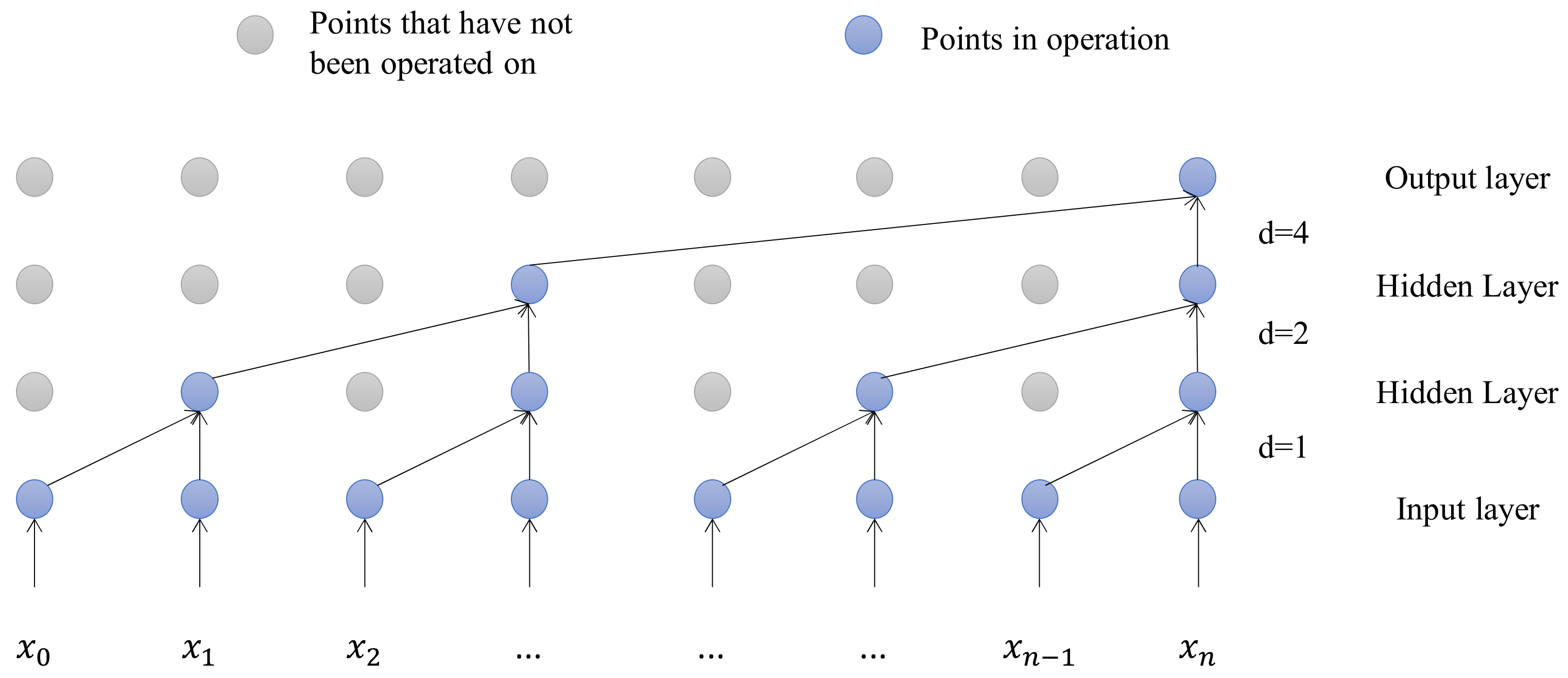
Temporal convolutional networks (TCN) are commonly used to solve time-series problems and have superior performance in extracting time-series correlations compared to traditional networks [33,34]. Their main structure is an inflated causal convolution, as shown in Figure 2.
In the article, feature extraction is performed through TCN, as shown in Figure 3.
First, a feature sequence of length n + 1 is fed into k TCN filters to obtain an intermediate matrix A * of size k × n , and this matrix consists of k column vectors of length n (i.e., A * = A 1 * , A 2 * , , A k * ). A specific element of each column vector is output as a sequence of features through the fully connected layer.

3.4. Improved Gated Recurrent Unit

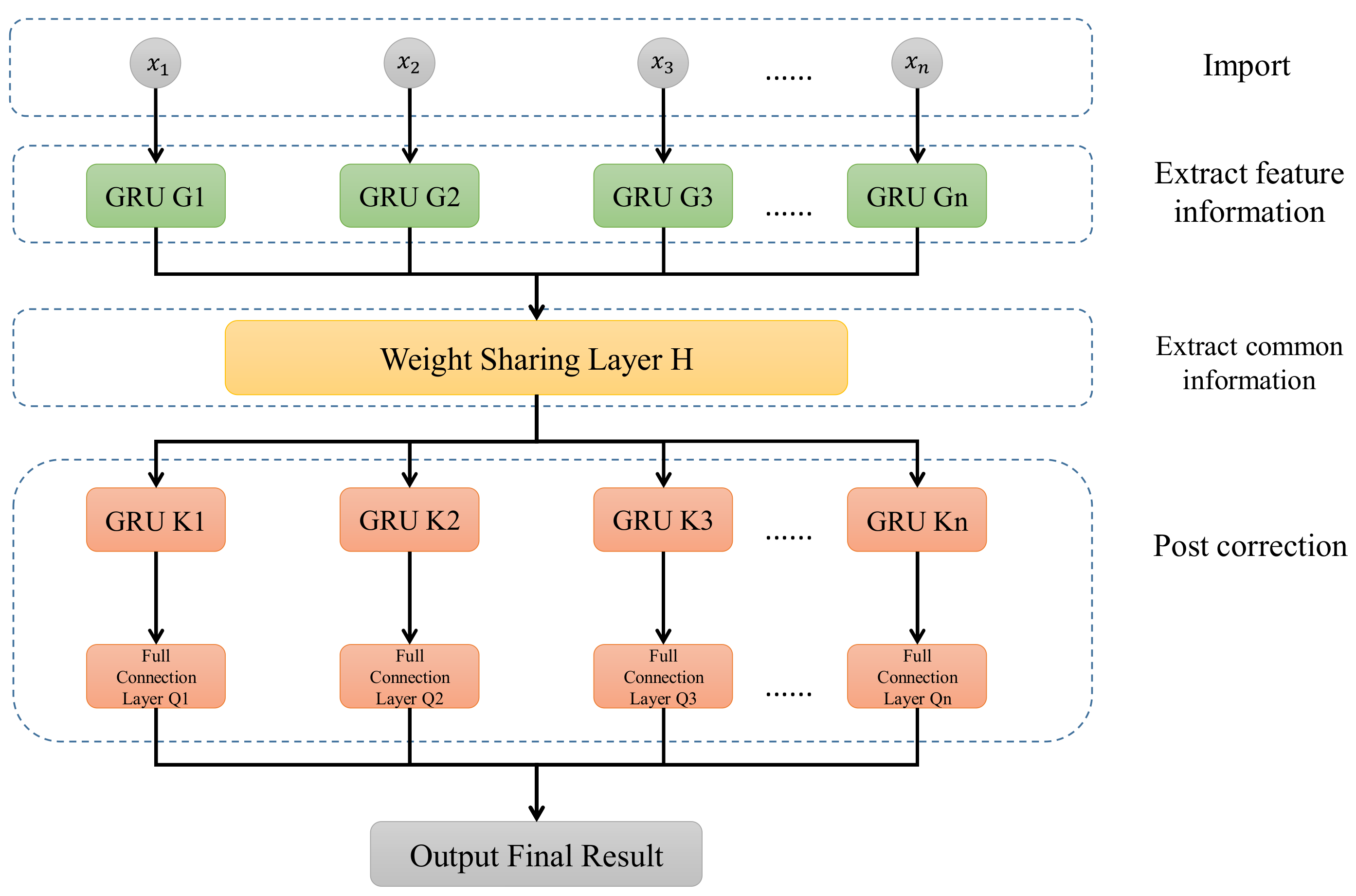
For machine learning algorithms with multiple feature inputs, the current mainstream training methods increase the computational effort of the multi-layer gated recurrent unit (GRU). To address this problem, the paper introduces a weight-sharing layer to the GRU, as shown in Figure 4.
The improved GRU essentially shares the intermediate structure of the tower GRU network, which not only ensures the compatibility of multidimensional data while retaining the input and output features of the original network, but also simplifies the network structure. By inputting each feature into the independent G-layer GRU in the front, it is trained and parsed independently; the weights are shared in the shared layer H to complete the extraction of the common information among the features; then, it enters the independent K-layer GRU in the back, which further explores the potential information among the features and makes the model have better learning ability for them; finally, the output is corrected through the fully connected layer Q. Compared with the ordinary GRU, the improved GRU reduces the number of feature inputs and the process of calculating feature weights, and simplifies the structure, so the efficiency is much higher than the ordinary GRU.
In summary, in order to address the imbalance in the number of different types of samples and further improve prediction accuracy and speed, a new scheme is proposed in this article. The overall prediction process is shown in Figure 5.
After filtering the input features using KPCA, the VMD was optimized using WOA to decompose each input feature into modal components in order to mine its regularity. The temporal features of the input information are extracted using TCN.
The samples were clustered using the K-means method according to the load characteristics, and after the load data had been clustered, the samples that accounted for a smaller percentage were expanded using SyMProD.
Predictions are made using an improved GRU, and an error correction model is constructed and trained, the results of which are used to compensate and improve prediction accuracy. The overall prediction process is shown in Figure 5.

4. Results and Discussions

4.1. Experimental Background and Evaluation Indicators

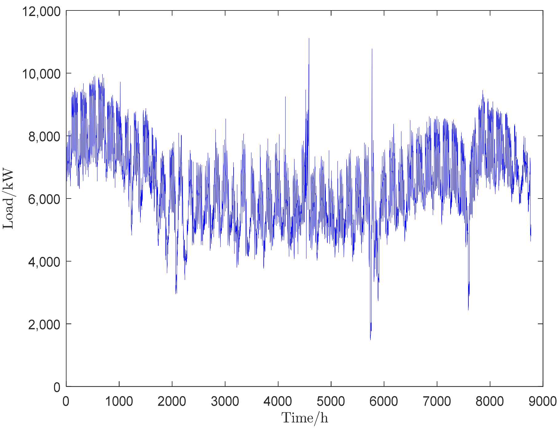
The dataset used in the paper is derived from partial load data from a European town for the years 2014–2015 and contains a total of approximately 9000 load data points with a sampling interval of 1 h (data span of approximately 1 year). The load data diagram is shown in Appendix B Figure A4. The data were divided into training and test sets in a 49:1 ratio, and the missing individual data were filled in using interpolation.
The mean absolute error (MAE), the mean absolute percentage error (MAPE), and the root mean square error (RMSE) were used to judge the evaluation indicators [35,36]. The MAE, MAPE and RMSE are shown in Equations (5)–(7).
X M A E = 1 n i = 1 n y i y ^ i
X M A P E = 100 % n i = 1 n y i y ^ i y i
X R M S E = 1 n i = 1 n y i y ^ i 2
In the above equation, n is the number of load data, y i is the true value of the data, and y ^ i is the predicted value of the data.

4.2. Feature Filtering Process

In the paper, KPCA was used to calculate the contribution rate of the input features to remove redundant features. The filtered features are shown in Appendix A Table A1.
As the three feature quantities of average temperature, relative humidity, and wind speed are strongly correlated, the concept of body temperature is introduced in the paper to combine these three features for calculation. This move can effectively reduce the amount of model training while retaining the input information and improving the prediction speed of the model. The general formula for body temperature is shown in Equations (8) and (9).
A T = 1.07 T + 0.2 E 0.65 V 2.7
E = 6.105 × R H × e 17.27 T 237.7 + T
where AT is the body temperature, T is the air temperature, E is the water vapor pressure, V is the average wind speed, and RH is the percentage of relative humidity. The contribution rate of body temperature was calculated to be 0.779, which is greater than the set threshold value of 0.5, so it can be used as an input feature to participate in model training. In summary, the input features after screening were four, namely body temperature, date type, precipitation, and illumination.
After determining the input feature items, perform VMD decomposition on each feature item. The input features and their decomposition results are shown in Appendix B Figure A5, Figure A6, Figure A7, Figure A8, Figure A9, Figure A10, Figure A11, Figure A12, Figure A13, Figure A14 and Figure A15.

4.3. SyMProD-Based Sample Expansion

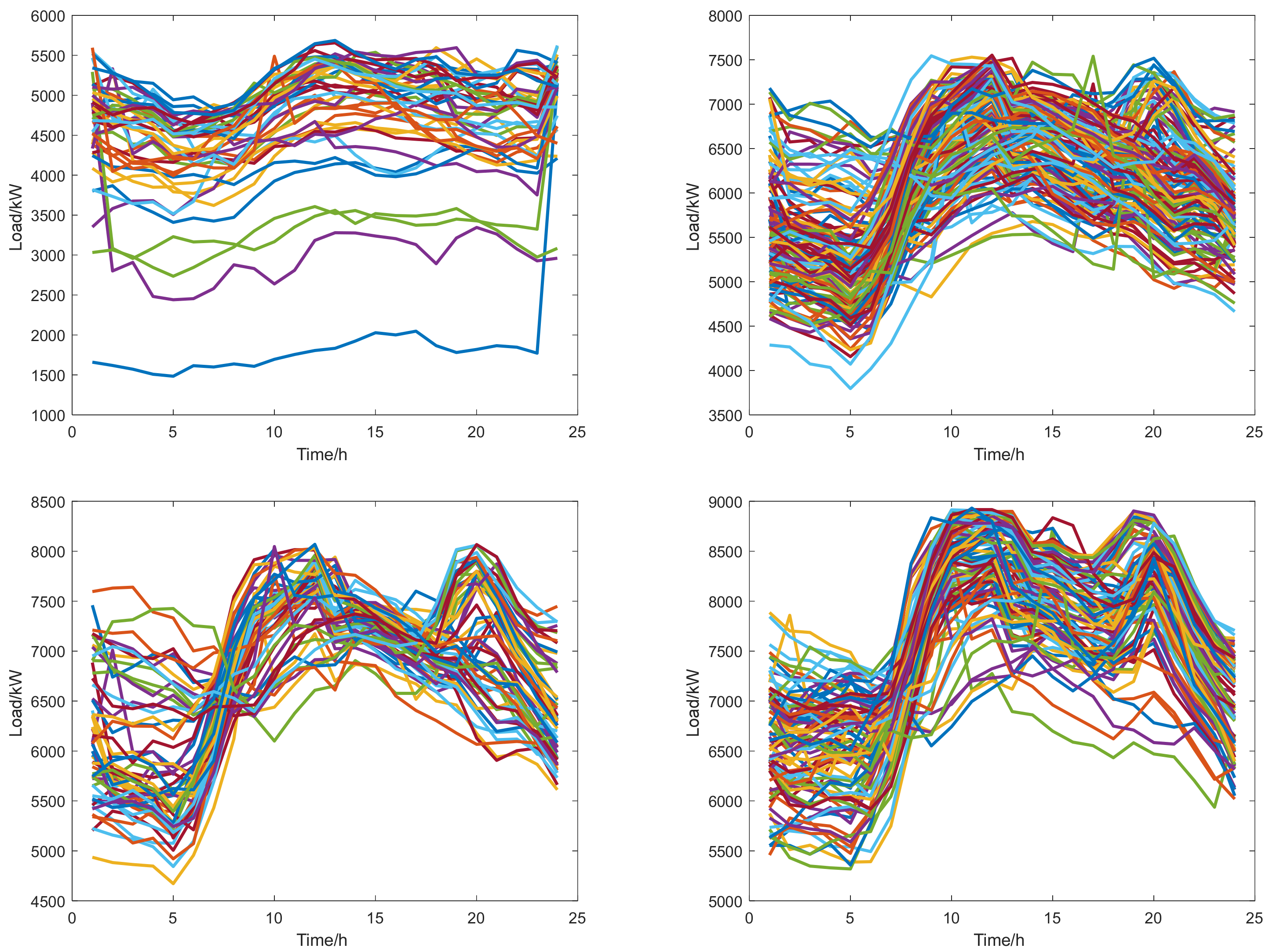
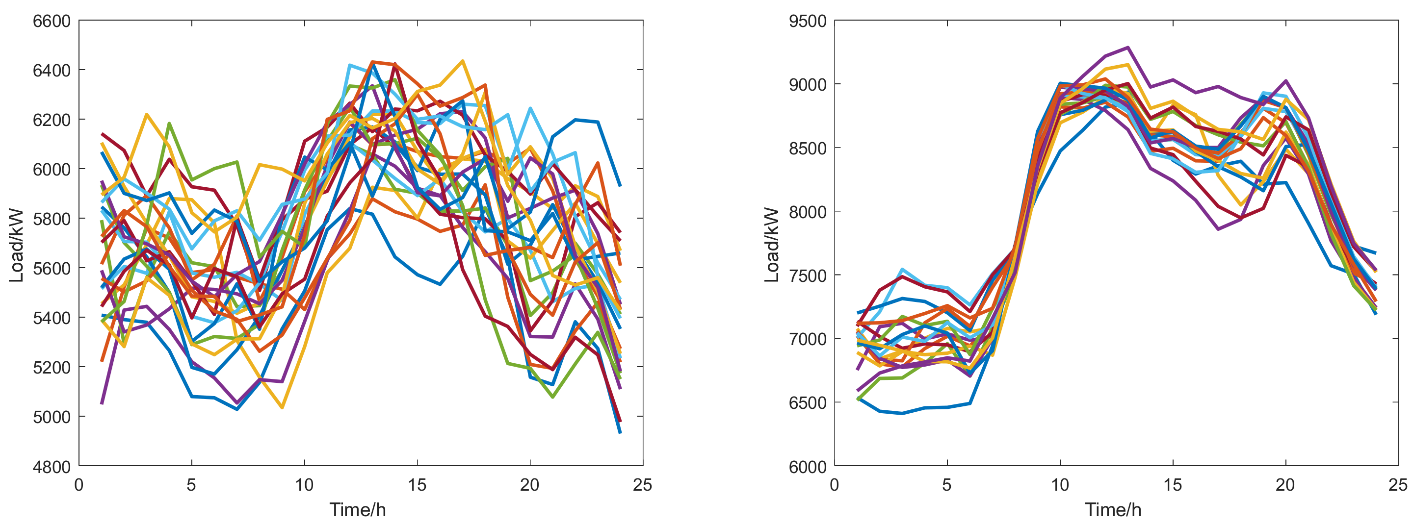
In this paper, the data is clustered using the K-means algorithm based on the average daily load. After clustering, the input data was clustered into six classes. Class 1 load profiles are mainly spring and autumn holidays without much heating or cooling demand and with minimal electricity consumption. Class 2 are mainly spring and autumn weekdays. Class 3 are mainly winter weekdays with high electricity demand. Class 4 are normal-temperature weekdays and high-temperature holidays in summer. Class 5 are mainly winter holidays with heating demand and low electricity consumption. Class 6 are high-temperature weekdays with the highest electricity consumption. The maximum load is significantly higher in the first five categories. In the original data, the ratio of samples of each type reached 43:126:57:92:28:19, with the ratio of the most to least samples exceeding 6:1 (i.e., the sample data of category 5 and category 6 are minority samples). After clustering, the general load samples are shown in Figure 6, and the minority samples are shown in Figure 7. The minority sample was expanded using SyMProD, and the data after the expansion was carried out are shown in Figure 8. The curves in Figure 6, Figure 7 and Figure 8 are only intended to enable readers to distinguish the approximate number of clusters (expansions) of various samples.
By comparing the images before and after sample expansion, it can be seen that using SyMProD to expand the samples can reduce the ratio of the maximum to minimum samples from the original 6:1 to about 3:1, effectively alleviating the problem of large differences in the number of training samples.

4.4. Experimental Results and Analysis

4.4.1. Algorithm Vertical Improvement Comparison Experiments

In order to consider the predictive power of the proposed method, the advantages of the method are highlighted by comparing it with several algorithms from the improvement process. The added algorithms and related settings are shown in Table 1. The runtime of each method shown in Table 1 is shown in Appendix A Table A2.
The prediction and error results for each of the methods above are shown in Figure 9 and Figure 10, with the arithmetic example containing approximately 180 data points, including approximately two minority sample days. The MAE, MAPE, and RMSE indicators for the general sample area and the area where the minority sample is located are shown in Table 2 and Table 3. A radar chart of MAPE values corresponding to these two tables is shown in Appendix A Figure A1 and Figure A2.
As seen from the above results, Method 1 is lacking in both data and feature processing, and therefore has the highest prediction error value in the case test. Method 2 uses a TCN network to extract the features, and compared to Method 1, the prediction error is significantly reduced, especially in some areas.
Method 3 further exploits the timing characteristics of the feature sequences by introducing the WOA-VMD algorithm and improving the GRU algorithm, resulting in a significant improvement in the running speed of the algorithm compared to Methods 1 and 2. However, since the minority sample expansion is not performed, there is still much room for improvement in the prediction results for the minority sample region.
Method 4 has a small number of sample expansions compared to Method 3, and the expanded sample data are added to the training set together, so the prediction effect in a small number of sample areas is greatly improved compared to Method 3, with an improvement in accuracy of about 59.41%; moreover, Method 4 introduces WOA optimization to the VMD, which effectively reduces the time used for tuning, so that the overall running time of Method 4 does not increase compared to that of Method 3, despite the additional small number of sample expansions. The overall running time of Method 4 did not increase compared to Method 3 with a few additional sample expansions.
In this article, all load-forecasting algorithms used are evaluated for their excellence by measuring their MAPE values. If its MAPE value is within 5%, it can be evaluated as “qualified”; within 3%, it can be rated as “good”; and within 1%, it can be rated as “excellent”. From Table 2 and Table 3, it can be seen that by improving the original algorithm, the prediction accuracy of the algorithm proposed in this article has reached the “excellent” level in both ordinary and minority regions.
The proposed method has the highest prediction accuracy and the shortest overall running time compared to the previous methods. By introducing new mechanisms such as feature filtering and error compensation, the prediction accuracy is significantly improved while the training efficiency is also significantly increased. Because of the improvements to the algorithm and the processing of the data, the overall running time of the methods proposed in the paper decreases rather than rises after several additional elements are performed. The training time for Method 1 is around 201 min, while the proposed method takes 170 min, a reduction of about 14.92% in training time and an improvement of about 80.24% in accuracy.

4.4.2. Algorithm Cross-Sectional Comparison Experiments

In order to highlight the superiority of the method proposed in the paper, it was compared with other commonly used algorithms. The algorithms and related settings used are shown in Table 4. The prediction results and errors for each method are shown in Figure 11 and Figure 12, and the arithmetic examples contain a total of approximately 180 data points. The MAE, MAPE, and RMSE metrics for each algorithm are shown in Table 5. A radar chart of MAPE values corresponding to the table is shown in Appendix A Figure A3.
From the above results, it can be seen that the operation results of the XGBoost model show that its various error values are high. LSTM, as one of the most commonly used neural networks, has a certain advantage in accuracy compared to XGBoost. LSSVM, as one of the prediction algorithms that has been developed and matured, finds a balance between prediction effect and training time for data with a not very large sample size. LightGBM, as an improved algorithm of XGBoost, has a considerable improvement in prediction accuracy.
In this article, all load-forecasting algorithms used are evaluated for their excellence by measuring their MAPE values. If its MAPE value is within 5%, it can be evaluated as “qualified”; within 3%, it can be rated as “good”; and within 1%, it can be rated as “excellent”. From Table 4 and Table 5, it can be seen that compared with other commonly used load-forecasting algorithms, the prediction accuracy of the proposed load forecasting algorithm in this paper can reach the “excellent” level under different samples, which proves that the algorithm in this paper has good universality under different data samples.
In summary, the proposed method demonstrates that feature filtering of the input data can effectively reduce the number of input features and improve the training speed of the model. Using WOA to optimize the VMD can minimize the tuning time of the VMD algorithm to improve the efficiency of the algorithm while ensuring the best parameters of the VMD. Improving the structure of the GRU can significantly reduce the training time while ensuring the prediction accuracy. Compensating for the errors generated during the training of the model can effectively improve the overall prediction accuracy. Expanding a small number of samples can significantly improve the prediction accuracy in a small number of sample areas. The improvement of the GRU architecture can significantly lower the training time while ensuring prediction accuracy. The compensation of the errors generated in the training of the model can effectively improve the overall prediction accuracy. The expansion of a few samples can significantly improve the prediction accuracy of a few sample areas. In addition, the comparison with similar algorithms and the use of different algorithms proves that the proposed load prediction method has excellent generality and prediction accuracy.

5. Conclusions

In this paper, a load-prediction method based on feature screening and error compensation under imbalanced samples is proposed by drawing on cutting-edge technologies in artificial intelligence and machine learning at home and abroad, and the following conclusions are drawn:
By filtering features, the number of input features can be effectively reduced, and the accuracy of prediction and training efficiency can be improved, while also ensuring the stability of the model. An error compensation model has been constructed, which can effectively improve the overall prediction accuracy of the model. Expanding a few samples can effectively improve the problem of imbalanced sample size and improve the prediction accuracy of minority sample areas. By improving existing algorithms, the existing problems have been solved, effectively reducing the time required for algorithm training, parameter adjustment, and more, and improving overall prediction efficiency.
In the future, key research will be conducted to address the issue of long computational time for this algorithm. At the same time, we will attempt to combine load-forecasting algorithms with big data platforms in order to achieve the function of “real-time prediction” in the industrial field.

Author Contributions

Z.W. completed the basic content of this article, and H.L. evaluated the feasibility of this article and made detailed modifications. All authors have read and agreed to the published version of the manuscript.

Funding

This research was supported by Shanghai Science and Technology Commission Key Program (grant no. 20dz1206100).

Data Availability Statement

Not applicable.

Conflicts of Interest

All authors claim that this study was conducted without any commercial or financial activities relationships that may be interpreted as potential conflicts of interest.

Appendix A

Table A1. Feature filtering process.
Serial NumberFeaturesContribution RateWhether to Retain (Threshold 0.5)
1Average temperature0.854Yes
2Humidity0.843Yes
3Wind speed0.732Yes
4Date Type0.712Yes
5Precipitation0.665Yes
6Illumination0.547Yes
7Pneumatic pressure0.331No
8Air visibility0.318No
9Air density0.201No
Table A2. Running time of each algorithm.
Main Algorithm RuntimeTotal Running Time (Including Time Consumed for Reference Adjustment)
Method 1VMD: 16 min
GRU: 141 min
201 min
Method 2VMD: 16 min
TCN: 47 min
GRU: 101 min
208 min
Method 3WOA-VMD: 23 min
TCN: 69 min
IGRU: 77 min
189 min
Method 4WOA-VMD: 23 min
TCN: 71 min
IGRU: 94 min
188 min
Method in this paperWOA-VMD: 23 min
TCN: 67 min
IGRU: 80 min
170 min
Figure A1. MAPE value of prediction results radar chart (vertical improvement comparison experiments).
Energies 16 04130 g0a1
Figure A2. MAPE value radar chart of prediction results in a few sample areas.
Energies 16 04130 g0a2
Figure A3. MAPE value of prediction results radar chart (cross-sectional comparison experiments).
Energies 16 04130 g0a3

Appendix B

Figure A4. Load data.
Energies 16 04130 g0a4
Figure A5. Average temperature.
Energies 16 04130 g0a5
Figure A6. Relative humidity.
Energies 16 04130 g0a6
Figure A7. Wind speed.
Energies 16 04130 g0a7
Figure A8. Date type.
Energies 16 04130 g0a8
Figure A9. Precipitation.
Energies 16 04130 g0a9
Figure A10. Illuminance.
Energies 16 04130 g0a10
Figure A11. Apparent temperature.
Energies 16 04130 g0a11
Figure A12. VMD for date type.
Energies 16 04130 g0a12
Figure A13. VMD for illuminance.
Energies 16 04130 g0a13
Figure A14. VMD for precipitation.
Energies 16 04130 g0a14
Figure A15. VMD for apparent temperature.
Energies 16 04130 g0a15

Appendix C

The experimental environment and computer configuration used in this article are as follows:
  • Experimental software: Python 3.8; Pycharm 2018
  • Experimental environment: PyTorch; Keras; Tensorflow
  • Computer configuration:
  • CPU: Intel i5 4200U
  • GPU: NVIDIA GT740M
  • RAM: 16 GB
  • Operating system: Windows 10 Professional Edition
The full name and abbreviation of proper nouns involved in this article (in their order of appearance in the main text):
  • Empirical mode decomposition (EMD)
  • Variational mode decomposition (VMD)
  • Whale optimization algorithm (WOA)
  • Long-short-term-memory (LSTM)
  • Gated recurrent unit (GRU)
  • Synthetic minority based on probabilistic distribution (SyMProD)
  • Kernel principal component analysis (KPCA)
  • Mean envelope entropy (MEE)
  • Temporal convolutional networks (TCN)
  • Mean absolute error (MAE)
  • Mean absolute percentage error (MAPE)
  • Root mean square error (RMSE)
  • Extreme gradient boost (XGBoost)
  • Light gradient boost machine (LightGBM)
  • Least squares support vector machine (LSSVM)

References

  1. Kong, W.; Dong, Z.Y.; Jia, Y.; Hill, D.J.; Xu, Y.; Zhang, Y. Short-Term Residential Load Forecasting Based on LSTM Recurrent Neural Network. IEEE Trans. Smart Grid 2017, 10, 841–851. [Google Scholar] [CrossRef]
  2. Dewangan, F.; Abdelaziz, A.Y.; Biswal, M. Load Forecasting Models in Smart Grid Using Smart Meter Information: A Review. Energies 2023, 16, 1404. [Google Scholar] [CrossRef]
  3. Zhang, X.; Wang, R.; Zhang, T.; Liu, Y.; Zha, Y. Short-Term Load Forecasting Using a Novel Deep Learning Framework. Energies 2018, 11, 1554. [Google Scholar] [CrossRef]
  4. Niu, D.; Yu, M.; Sun, L.; Gao, T.; Wang, K. Short-term multi-energy load forecasting for integrated energy systems based on CNN-BiGRU optimized by attention mechanism. Appl. Energy 2022, 313, 118801. [Google Scholar] [CrossRef]
  5. Wu, H.; Liang, Y.; Heng, J. Pulse-diagnosis-inspired multi-feature extraction deep network for short-term electricity load forecasting. Appl. Energy 2023, 339, 120995. [Google Scholar] [CrossRef]
  6. Mounir, N.; Ouadi, H.; Jrhilifa, I. Short-term electric load forecasting using an EMD-BI-LSTM approach for smart grid energy management system. Energy Build. 2023, 288, 113022. [Google Scholar] [CrossRef]
  7. Li, J.; Deng, D.; Zhao, J.; Cai, D.; Hu, W.; Zhang, M.; Huang, Q. A Novel Hybrid Short-Term Load Forecasting Method of Smart Grid Using MLR and LSTM Neural Network. IEEE Trans. Ind. Inform. 2021, 17, 2443–2452. [Google Scholar] [CrossRef]
  8. Su, J.; Han, X.; Hong, Y. Short Term Power Load Forecasting Based on PSVMD-CGA Model. Sustainability 2023, 15, 2941. [Google Scholar] [CrossRef]
  9. Wang, Y.; Zhang, W.; Li, X.; Wang, A.; Wu, T.; Bao, Y. Monthly Load Forecasting Based on an ARIMA-BP Model: A Case Study on Shaoxing City. In Proceedings of the 2020 12th IEEE PES Asia-Pacific Power and Energy Engineering Conference (APPEEC), Nanjing, China, 20–23 September 2020; pp. 1–6. [Google Scholar]
  10. Wang, Y.; Zhang, N.; Chen, X. A Short-Term Residential Load Forecasting Model Based on LSTM Recurrent Neural Network Considering Weather Features. Energies 2021, 14, 2737. [Google Scholar] [CrossRef]
  11. Yuan, J.; Wang, L.; Qiu, Y.; Wang, J.; Zhang, H.; Liao, Y. Short-term electric load forecasting based on improved Extreme Learning Machine Mode. Energy Rep. 2021, 7, 1563–1573. [Google Scholar] [CrossRef]
  12. Huang, N.E.; Shen, Z.; Long, S.R.; Wu, M.C.; Shih, H.H.; Zheng, Q.; Yen, N.-C.; Tung, C.C.; Liu, H.H. The empirical mode decomposition and the Hilbert spectrum for nonlinear and non-stationary time series analysis. Proc. R. Soc. London. Ser. A Math. Phys. Eng. Sci. 1998, 454, 903–995. [Google Scholar] [CrossRef]
  13. Zhou, Y.; Lin, Q.; Xiao, D. Application of LSTM-LightGBM Nonlinear Combined Model to Power Load Forecasting. J. Phys. Conf. Ser. 2022, 2294, 012035. [Google Scholar] [CrossRef]
  14. Meng, Z.; Xie, Y.; Sun, J. Short-term load forecasting using neural attention model based on EMD. Electr. Eng. 2021, 104, 1857–1866. [Google Scholar] [CrossRef]
  15. Zheng, H.; Yuan, J.; Chen, L. Short-Term Load Forecasting Using EMD-LSTM Neural Networks with a Xgboost Algorithm for Feature Importance Evaluation. Energies 2017, 10, 1168. [Google Scholar] [CrossRef]
  16. Dragomiretskiy, K.; Zosso, D. Variational Mode Decomposition. IEEE Trans. Signal Process. 2014, 62, 531–544. [Google Scholar] [CrossRef]
  17. Wang, N.; Li, Z. Short term power load forecasting based on BES-VMD and CNN-Bi-LSTM method with error correction. Front. Energy Res. 2023, 10, 1076529. [Google Scholar] [CrossRef]
  18. Xu, C.; Chen, H.; Xun, W.; Zhou, Z.; Liu, T.; Zeng, Y.; Ahmad, T. Modal decomposition based ensemble learning for ground source heat pump systems load forecasting. Energy Build. 2019, 194, 62–74. [Google Scholar] [CrossRef]
  19. Wang, S.; Wei, L.; Zeng, L. Ultra-short-term Photovoltaic Power Prediction Based on VMD-LSTM-RVM Model. IOP Conf. Series Earth Environ. Sci. 2021, 781, 042020. [Google Scholar] [CrossRef]
  20. Wei, J.; Wu, X.; Yang, T.; Jiao, R. Ultra-short-term forecasting of wind power based on multi-task learning and LSTM. Int. J. Electr. Power Energy Syst. 2023, 149, 109073. [Google Scholar] [CrossRef]
  21. Semmelmann, L.; Henni, S.; Weinhardt, C. Load forecasting for energy communities: A novel LSTM-XGBoost hybrid model based on smart meter data. Energy Inform. 2022, 5, 24. [Google Scholar] [CrossRef]
  22. Hua, H.; Liu, M.; Li, Y.; Deng, S.; Wang, Q. An ensemble framework for short-term load forecasting based on parallel CNN and GRU with improved ResNet. Electr. Power Syst. Res. 2023, 216, 109057. [Google Scholar] [CrossRef]
  23. Chen, Z.; Jin, T.; Zheng, X.; Liu, Y.; Zhuang, Z.; Mohamed, M.A. An innovative method-based CEEMDAN–IGWO–GRU hybrid algorithm for short-term load forecasting. Electr. Eng. 2022, 104, 3137–3156. [Google Scholar] [CrossRef]
  24. Lv, L.; Wu, Z.; Zhang, J.; Zhang, L.; Tan, Z.; Tian, Z. A VMD and LSTM Based Hybrid Model of Load Forecasting for Power Grid Security. IEEE Trans. Ind. Inform. 2021, 18, 6474–6482. [Google Scholar] [CrossRef]
  25. Inteha, A.; Al Masood, N. A GRU-GA Hybrid Model Based Technique for Short Term Electrical Load Forecasting. In Proceedings of the 2nd International Conference on Robotics, Electrical and Signal Processing Techniques (ICREST), Dhaka, Bangladesh, 5–7 January 2021; pp. 515–519. [Google Scholar] [CrossRef]
  26. Yang, T.; Huang, L.; Fu, P.; Chen, X.; Zhang, X.; Chen, T.; He, S. Distributed energy power prediction of the variational modal decomposition and Gated Recurrent Unit optimization model based on the whale algorithm. Energy Rep. 2022, 8, 24–33. [Google Scholar] [CrossRef]
  27. Yu, M.; Niu, D.; Gao, T.; Wang, K.; Sun, L.; Li, M.; Xu, X. A novel framework for ultra-short-term interval wind power prediction based on RF-WOA-VMD and BiGRU optimized by the attention mechanism. Energy 2023, 269, 126738. [Google Scholar] [CrossRef]
  28. Kunakorntum, I.; Hinthong, W.; Phunchongharn, P. A Synthetic Minority Based on Probabilistic Distribution (SyMProD) Oversampling for Imbalanced Datasets. IEEE Access 2020, 8, 114692–114704. [Google Scholar] [CrossRef]
  29. Zhu, A.; Zhao, Q.; Yang, T.; Zhou, L.; Zeng, B. Condition monitoring of wind turbine based on deep learning networks and kernel principal component analysis. Comput. Electr. Eng. 2023, 105, 108538. [Google Scholar] [CrossRef]
  30. Fan, Y.; Wang, H.; Zhao, X.; Yang, Q.; Liang, Y. Short-Term Load Forecasting of Distributed Energy System Based on Kernel Principal Component Analysis and KELM Optimized by Fireworks Algorithm. Appl. Sci. 2021, 11, 12014. [Google Scholar] [CrossRef]
  31. Tao, C.; Lu, J.; Lang, J.; Peng, X.; Cheng, K.; Duan, S. Short-Term Forecasting of Photovoltaic Power Generation Based on Feature Selection and Bias Compensation–LSTM Network. Energies 2021, 14, 3086. [Google Scholar] [CrossRef]
  32. Mirjalili, S.; Lewis, A. The Whale Optimization Algorithm. Adv. Eng. Softw. 2016, 95, 51–67. [Google Scholar] [CrossRef]
  33. Luo, W.; Dou, J.; Fu, Y.; Wang, X.; He, Y.; Ma, H.; Wang, R.; Xing, K. A Novel Hybrid LMD–ETS–TCN Approach for Predicting Landslide Displacement Based on GPS Time Series Analysis. Remote. Sens. 2022, 15, 229. [Google Scholar] [CrossRef]
  34. Ma, Q.; Wang, H.; Luo, P.; Peng, Y.; Li, Q. Ultra-short-term Railway traction load prediction based on DWT-TCN-PSO_SVR combined model. Int. J. Electr. Power Energy Syst. 2021, 135, 107595. [Google Scholar] [CrossRef]
  35. Wang, Y.; Chen, J.; Chen, X.; Zeng, X.; Kong, Y.; Sun, S.; Guo, Y.; Liu, Y. Short-Term Load Forecasting for Industrial Customers Based on TCN-LightGBM. IEEE Trans. Power Syst. 2020, 36, 1984–1997. [Google Scholar] [CrossRef]
  36. He, L.; Li, Z.; Xie, Y.; Liu, Y.; Liu, M. Buckling failure mechanism and critical buckling load prediction method of super-long piles in soft-clay ground in deep water. Ocean Eng. 2023, 276, 114216. [Google Scholar] [CrossRef]
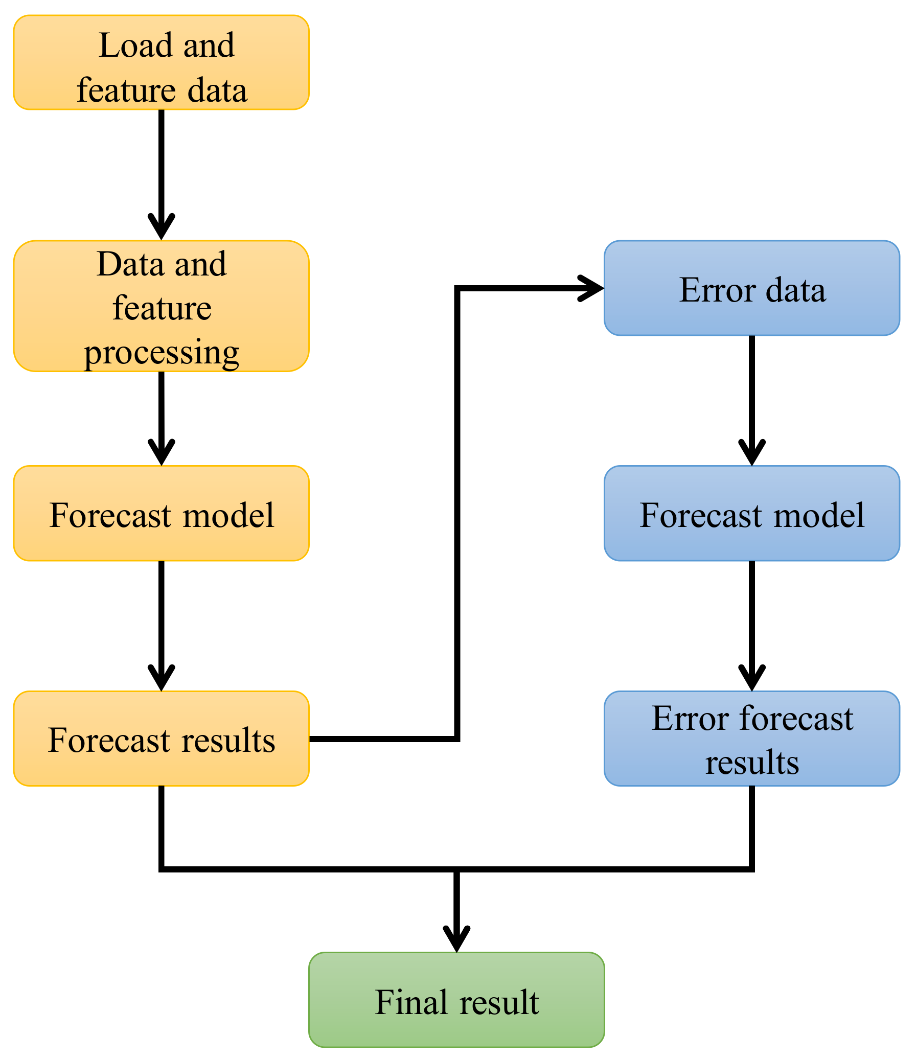
Figure 1. Error compensation process.
Energies 16 04130 g001
Figure 2. Dilated convolution structure.
Energies 16 04130 g002
Figure 3. TCN feature extraction process.
Energies 16 04130 g003
Figure 4. Flow chart of improving GRU.
Energies 16 04130 g004
Figure 5. Overall prediction process.
Energies 16 04130 g005
Figure 6. Clustered ordinary load samples (categories 1 to 4).
Energies 16 04130 g006
Figure 7. Clustered minority load samples (category 5 and 6).
Energies 16 04130 g007
Figure 8. Expanded sample (category 5 and 6).
Energies 16 04130 g008
Figure 9. Comparison of prediction results of various methods (vertical improvement comparison experiments).
Energies 16 04130 g009
Figure 10. Comparison of error results of various methods (vertical improvement comparison experiments).
Energies 16 04130 g010
Figure 11. Comparison of prediction results of various methods (cross-sectional comparison experiments).
Energies 16 04130 g011
Figure 12. Comparison of error results of various methods (cross-sectional comparison experiments).
Energies 16 04130 g012
Table 1. Algorithm and settings (vertical improvement comparison experiments).
Algorithm UsedAlgorithm Settings
Method 1VMD-GRU algorithmNeurons: 128
Activation function: RELU
Learning rate: 0.01
Training style: Adam
Method 2VMD-TCN-GRU algorithmNeurons: 128
Activation function: RELU
Learning rate: 0.01
Training style: Adam
Method 3WOA-VMD-TCN-improved GRU algorithmNeurons: 128
Activation function: RELU
Learning rate: 0.01
Training style: Adam
Method 4WOA-VMD-TCN-improved GRU algorithm (for minority sample expansion)Neurons: 128
Activation function: RELU
Learning rate: 0.01
Training style: Adam
Method in this paperWOA-VMD-TCN-improved GRU algorithm (for minority sample expansion and feature screening to construct error compensation models)Neurons: 128
Activation function: RELU
Learning rate: 0.01
Training style: Adam
Table 2. Prediction error of each algorithm (vertical improvement comparison experiments).
MAE/kWMAPE/%RMSE/kW
Method 1263.3934.13417.397
Method 2250.3053.87302.359
Method 3194.9163.18310.693
Method 4108.3731.72177.442
Method in this paper61.7790.9784.637
Table 3. Prediction error of each algorithm in a few sample areas.
MAE/kWMAPE/%RMSE/kW
Method 1599.4628.98936.248
Method 2441.1056.61479.568
Method 3318.0294.73416.602
Method 4128.2231.92297.485
Method in this paper38.5860.5845.825
Table 4. Algorithm and settings (cross-sectional comparison experiments).
Algorithm UsedAlgorithm-Related Settings
Method 1Extreme gradient boost (XGBoost)algorithmNumber of trees: 100
Maximum tree depth: 20
Leaf nodes: 40
Method 2Light gradient boost machine (LightGBM) algorithmNumber of trees: 100
Maximum tree depth: 20
Leaf nodes: 40
Method 3Least squares support vector machine (LSSVM) algorithmKernel function: RBF
Learning rate: 0.01
Method 4LSTM algorithmNeurons: 128
Activation function: RELU
Learning rate: 0.01
Training style: Adam
Method in this paperWOA-VMD-TCN-improved GRU algorithm (method in this paper)Neurons: 128
Activation function: RELU
Learning rate: 0.01
Training style: Adam
Table 5. Prediction error of each algorithm (cross-sectional comparison experiments).
MAE/kWMAPE/%RMSE/kW
Method 1124.0532.53153.771
Method 298.3121.82123.594
Method 394.0521.79119.776
Method 486.3511.57108.573
Method in this paper50.5610.9667.511
Disclaimer/Publisher’s Note: The statements, opinions and data contained in all publications are solely those of the individual author(s) and contributor(s) and not of MDPI and/or the editor(s). MDPI and/or the editor(s) disclaim responsibility for any injury to people or property resulting from any ideas, methods, instructions or products referred to in the content.