An Early Fault Detection Method for Wind Turbine Main Bearings Based on Self-Attention GRU Network and Binary Segmentation Changepoint Detection Algorithm

Abstract

The condition monitoring and potential anomaly detection of wind turbines have gained significant attention because of the benefits of reducing the operating and maintenance costs and enhancing the reliability of wind turbines. However, the complex and dynamic operation states of wind turbines still pose tremendous challenges for reliable and timely fault detection. To address such challenges, in this study, a condition monitoring approach was designed to detect early faults of wind turbines. Specifically, based on a GRU network with a self-attention mechanism, a SAGRU normal behavior model for wind turbines was constructed, which can learn temporal features and mine complicated nonlinear correlations within different status parameters. Additionally, based on the residual sequence obtained using a well-trained SAGRU, a binary segmentation changepoint detection algorithm (BinSegCPD) was introduced to automatically identify deterioration conditions in a wind turbine. A case study of a main bearing fault collected from a 50 MW windfarm in southern China was employed to evaluate the proposed method, which validated its effectiveness and superiority. The results showed that the introduction of a self-attention mechanism significantly enhanced the model performance, and the adoption of a changepoint detection algorithm improved detection accuracy. Compared to the actual fault time, the proposed approach could automatically identify the deterioration conditions of main bearings 72.47 h in advance.

1. Introduction

With the increasing depletion of petrochemical energy, wind energy, as one of the most promising forms of renewable energy resources for generating big amounts of electricity, has gained worldwide attention [1,2]. However, the majority of wind turbine installations are in isolated locations such as mountains and deserts, and generally operate under hostile weather conditions and complex geographical environments, causing continual faults and unexpected shutdowns [3]. Low reliability and high maintenance costs severely affect the generation performance of wind turbines, and also have a great influence on the economic benefits of windfarm operators, hindering the constructive development of the wind power industry [4,5]. According to the statistics, the operation and maintenance (O&M) costs for onshore wind turbines account for approximately 10–15% of the total production cost, while accounting for as high as 20–30% for offshore wind turbines [6]. Therefore, to reduce the O&M costs and minimize the economic loss, it is crucial and valuable to investigate advanced condition monitoring methods for early potential fault detection, which can further prevent secondary damages or even disastrous accidents, such as fire and tower collapse [7].

Numerous technologies have been used in recent years to monitor the operating status of wind turbines, which may be mainly categorized into physical-model-based methods and data-driven approaches. Physical model methods have been demonstrated to be successful and are frequently employed, typically including the parity equation [8], Kalman filter theory [9], and observation-based technology [10,11]. However, in practical engineering, it is difficult to build a precise mathematic model because of the complicated electromechanical structure and extremely varied operation status of wind turbines, which, to a significant extent, set limitations on the ongoing improvement and use of physical model methods.

Different from physical model methods, data-driven approaches merely rely on recorded operating data and do not require much physical knowledge or precise mathematics models, which have attracted considerable attention in the field of condition monitoring of wind turbines. Based on different measured signals, data-driven methods can be generally classified as follows:

(1)

Vibration monitoring [12,13,14,15], oil analysis [16,17], acoustic emission monitoring [18], etc. Although these methods have become commonly used technologies for wind turbine fault detection, they are costly and complicated in their actual application because of the installation of extra devices, including additional sensors and data-collecting hardware.

(2)

Methods using operating data recorded on a supervisory control and data acquisition (SCADA) system. Currently, almost all large-scale wind turbines are installed with a SCADA system to collect and store tremendous amounts of operation state data, including meteorological environment (e.g., air pressure, air temperature, air humidity, wind direction, wind speed), temperature, pressure, and electrical parameters. Therefore, due to the advantages of accessibility to massive monitoring data, SCADA-data-driven approaches have been found to be cost effective and highly efficient, and are extensively utilized in the realm of condition monitoring and potential fault detection (CMFD) of wind turbines [19,20,21,22].

Based on SCADA data, machine learning or deep learning algorithms, such as support vector machine (SVM) [23], backpropagation neural network (BPNN) [24], restricted Boltzmann machine (RBM) [25], Gaussian process [26], XGBoost [4,27], and autoencoder (AE) [28,29], have been employed to establish normal behavior models (NBMs) to detect potential faults for wind turbines. Dhiman HS et al. [23] built a data-driven early fault warning method for a wind turbine gearbox using the twin support vector machine (TWSVM). Comparison results demonstrated that the proposed method was superior in performance and reliability. Sun P et al. [24] designed a generalized model to identify deterioration conditions of wind turbines based on backpropagation neural networks (BPNNs) using SCADA data. The case study results illustrated that the designed approach performed better in wind turbine anomaly detection than conventional approaches. Yang W et al. [25] constructed an unsupervised anomaly detection method for wind turbine condition monitoring using a spatiotemporal pattern network (STPN) and stacked restricted Boltzmann machine (RBM). Case studies on three datasets illustrated that the designed method could detect the anomalies without the need for labeling data. Infield D et al. [26] introduced a SCADA-based potential anomaly detection approach for wind turbines using a Gaussian process (GP). Tao T et al. [27] designed a reliable and efficient blade-icing-detection approach for wind turbines based on hybrid features and a stacked XGBoost using SCADA data. Renström N et al. [28] designed a condition monitoring framework based on an autoencoder (AE) using the SCADA data and investigated various hyperparameters that affected the model’s performance. Chen J et al. [29] proposed a method for identifying anomalies of wind turbines based on multivariate analysis using stacked denoising autoencoders (SDAEs).

However, the above methods are all based on the hypothesis that SCADA data are independent and identically distributed (i.i.d.), but do not take into consideration the fact that SCADA data are essentially a time series.

Recurrent neural networks (e.g., RNN, LSTM, and GRU) have short-term memory capabilities due to their special network structure and are better at processing timeseries data, which have gained widespread attention in the realm of wind turbine condition monitoring and fault detection (CMFD) [30,31,32,33]. Zhang J et al. [30] employed long short-term memory networks (LSTM) to predict the active power of wind turbines and study the characteristics of the error distribution using the Gaussian mixture model (GMM). Lei J et al. [31] designed another novel detection approach using an end-to-end long short-term memory (LSTM) network. A condition monitoring (CM) method based on long short-term memory (LSTM) and an auto-encoder (AE) neural network was constructed by Chen H et al. [32] to evaluate wind turbine operation conditions. Convolutional neural networks (CNNs) and gated recurrent unit (GRU) networks were employed to mine spatial–temporal feature information from SCADA data to create Kong Z et al.’s [33] innovative approach for monitoring the state of wind turbines.

In summary, numerous studies on approaches for potential fault detection of wind turbines utilizing SCADA data have been widely conducted and proved to be effective; however, the following limitations still need to be addressed:

(1)

The previous studies do not take the temporal characteristics of SCADA operating data into account, and monitoring variables obtained by feature selection are assigned identical weights before being fed into the models, so they cannot fully extract sophisticated spatial–temporal features, thus leading to unsatisfactory model performance.

(2)

At present, for predicted residual time series, the fixed threshold or adaptive threshold used in the existing research may lead to missed detection or false alarm due to the excessively large or too small thresholds. Therefore, by combining with other statistical analysis methods, there is still space for improvement in the accuracy and reliability of anomaly detection.

Consequently, to solve the above issues, based on the self-attention (SA) mechanism [34], GRU networks, and a binary segmentation change-point detection (BinSegCPD) algorithm [35,36], an innovative wind turbine condition monitoring method (SAGRU–BinSegCPD) was designed in this study, whose principal contributions are as follows:

(1)

Through utilizing SCADA data, a normal behavior model (NBM) for wind turbines was constructed for condition monitoring using GRU networks with a self-attention mechanism, which has a powerful nonlinear modeling capability and can capture complicated temporal characteristics among the monitoring variables, thus enhancing the prediction performance.

(2)

To enhance the reliability and accuracy of early fault detection of wind turbines, the BinSegCPD algorithm was introduced to implement real-time change-point detection using prediction residual sequences. Additionally, we can achieve the automatic identification of deterioration status of wind turbines to decrease the high rate of false alarms or missed detections caused by a too large or too small threshold. As far as we know, this is the first application of the BinSegCPD algorithm in the field of wind turbine early fault detection.

(3)

Additionally, a real case of main-bearing-over-temperature fault of a wind turbine was utilized to verify the effectiveness and superiority of the designed SAGRU–BinSegCPD condition monitoring approach compared to other methods.

The rest of this paper is structured as follows: The framework of the designed SAGRU–BinSegCPD wind turbine condition monitoring method is briefly presented in Section 2. The normal behavior model based on SAGRU networks is thoroughly introduced in Section 3. In Section 4, the detection strategies for wind turbine early faults are described, including threshold alarm strategy and change-point detection algorithm. In Section 5, the designed SAGRU–BinSegCPD approach is verified, analyzed, and compared through using the SCADA data obtained from multiple wind turbines located in southern China, followed by a brief conclusion in Section 6.

2. Proposed SAGRU–BinSegCPD Method Framework

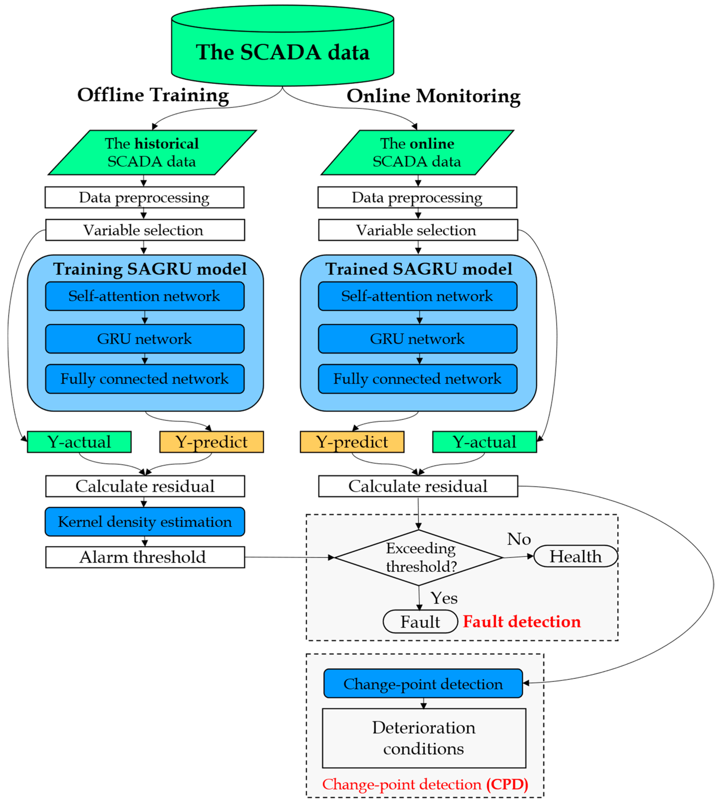
The overall framework of the designed SAGRU–BinSegCPD condition monitoring approach for wind turbines is shown in Figure 1, which primarily comprises two phases: offline training and online monitoring.

Phase 1—Offline Training: In this phase, utilizing the historical SCADA data collected from wind turbines under normal operating states, the proposed SAGRU normal behavior model of wind turbine key components for anomaly detection is trained. The following is a detailed description of the specific training steps:

Step 1: Data preprocessing and variable selection. It is worth noting that essential preprocessing steps, including data cleaning, data normalization, and variable selection, should be performed on the raw SCADA operating data, so as to obtain healthy datasets for model training.

Step 2: SAGRU model training. The healthy datasets acquired from step 1 are split into three sub-datasets for model training, model validation, and model testing. Based on the sub-datasets, we can obtain a well-trained SAGRU wind turbine normal behavior model, which can generate prediction outputs and the corresponding residuals.

Step 3: Residual analysis and alarm threshold. Based on the kernel density estimation algorithm (KDE), the statistical analysis is performed on the residual sequence produced using the SAGRU model in step 2. Therefore, for wind turbines operating under normal conditions, the probability density function (PDF) of the predicted residual can be fitted, and then an alarm threshold can be calculated for early fault detection and warning.

It should be noted that, considering the influence of seasonal climate, the training of the proposed model requires a large amount of normal operation data of wind turbines (at least one year). For a newly established windfarm having operated less than one year, the amount of SCADA data is not enough to support the model’s training. Therefore, the transfer learning method is adopted to train the model for the new windfarm. Firstly, pretrain the model by using the SCADA data of the same type of wind turbine in wind farms that have been in operation for longer time (more than one year); then, finetune the model parameters by using the SCADA date of the target windfarm.

Phase 2—Online Monitoring: In this phase, based on the well-trained SAGRU model obtained in phase 1, for the new incoming SCADA data, we can similarly obtain the prediction outputs and the prediction residuals. Then, the deterioration condition of wind turbines can be automatically identified using the BinSegCPD algorithm, and the latent anomalies are detected ahead of time through using the alarm threshold set in step 3. The detailed steps of online monitoring are described as follows:

Step 4: Deterioration condition identification. Based on the residual sequence produced by the well-trained SAGRU model, a real-time change-point detection could be carried out to distinguish the deterioration conditions of wind turbines.

Step 5: Early fault warning. In addition to the change-point detection implemented in step 4, alarm signals can be triggered when the predicted residual continuously exceeds the alarm threshold calculated by statistical analyses.

Consequently, combining the threshold alarm described in step 4 and the change-point detection presented in step 5, a hybrid anomaly detection strategy is introduced, which can increase the reliability of anomaly detection and alert the windfarm operation and maintenance technicians to take appropriate measures in a timely manner to avoid major faults.

3. Proposed SAGRU Normal Behavior Model

3.1. Data Preprocessing and Feature Selection

3.1.1. Data Cleaning

Due to the dynamic operating characteristics and sophisticated electromechanical structure of wind turbines, the SCADA system collects and stores massive high-dimensional operating data, including normal data and abnormal data caused by shutdowns, faults, turbulence, and device failures (e.g., devices of acquisition, communication, and storage). Therefore, to obtain healthy datasets for model training, it is necessary to implement data cleaning on the raw datasets before modeling.

A commonly used data-cleaning method, the quartile algorithm (QA), was employed to remove outliers and its detailed description is as follows:

In statistics, for a given ascending dataset, quartiles are the set of values that have three points dividing the dataset into four identical parts. Thus, there are three main quartiles, first, second, and third, represented by $Q_1$, $Q_2$, and $Q_3$, respectively. Here, $Q_3$, the upper quartile, represents the median of the upper half of the dataset, whereas $Q_1$, the lower quartile, refers to the lower half of the dataset. Additionally, $Q_2$ represents the median of the dataset.

The difference between the upper and lower quartiles is known as the interquartile range ($I_{\mathit{QR}}$), which can be calculated using Equation (1).

$$I_{\mathit{QR}}=Q_3-Q_1$$

(1)

Furthermore, the upper and lower thresholds for normal data can be calculated using the interquartile range $I_{\mathit{QR}}$ and Equation (2).

$$\left\{\begin{array}{c}{T}_L=Q_1-{1.5I}_{\mathit{QR}}\\ T_U=Q_3+{1.5I}_{\mathit{QR}}\end{array}\right.$$

(2)

In other words, data beyond the threshold $\left[T_L,T_U\right]$ should be treated as outliers and eliminated from the raw datasets.

3.1.2. Data Normalization

Generally, different variables have different dimensions. Thus, in order to decrease the difficulty of model training through eliminating the dimension effects, it is necessary to normalize these input measurements to narrow the value range to [0, 1] in accordance with Equation (3).

$$X^{\prime }=\frac{X-\mathit{min}\left(X\right)}{\mathit{max}\left(X\right)-\mathit{min}\left(X\right)}$$

(3)

where X is the raw data and max (X) and min (X) denote its maximum and minimum values.

3.1.3. Variable Selection

Normally, the SCADA system acquires and stores hundreds of operation state parameters for wind turbines, including continuous parameters (e.g., wind speed, active power, main bearing temperature, gearbox oil temperature, etc.) and discrete information (startups, shutdowns, fault records, etc.). Considering the model complexity and computing efficiency, status parameters having a high correlation with the target output (e.g., main bearing temperature) ought to be selected as model inputs.

For variable selection, there are three typical correlation calculation methods, namely the Spearman, Pearson, and Kendall correlation coefficients (SCC, PCC, KCC), which are statistics for calculating the monotonicity, linearity, and dependence different state parameters, respectively.

In this study, as a nonparametric measure of rank correlation (i.e., statistical dependence of ranking between two variables), the SCC was employed to select the modeling input variables, which can be calculated using Equation (4).

$$R_s=1-\frac{6\Sigma d_i^2}{n\left(n^2-1\right)}$$

(4)

where n represents the two variables’ data length, and d_i is the difference between the two variables in ranks of the “ith” elements.

Statistically [37], |R_s| < 0.3 indicates a weak correlation between variables; 0.3 < |R_s| < 0.7 indicates a moderate correlation between variables; and |R_s| > 0.7 indicates a strong correlation between variables. In this study, we directly chose 0.3 as the threshold value of R_s, based on which, we carried out the variable selection procedure.

3.2. Structure and Theory of the Designed SAGRU Model

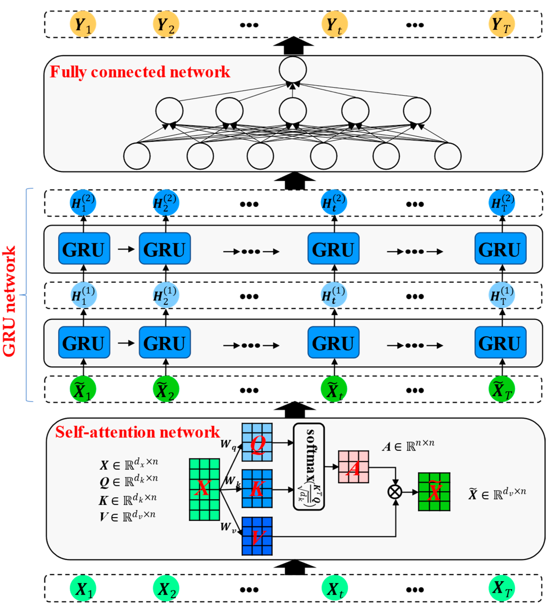
As depicted in Figure 2, the structure of the designed normal behavior model (SAGRU) for wind turbines mainly contains three parts: the self-attention (SA) network, the gated recurrent unit (GRU) network, and the fully connected (FC) network.

Part 1—Self-attention network: for minibatches of offline or online SCADA data (denoted as ${\mathit{X}}_1,{\mathit{X}}_2,\dots ,{\mathit{X}}_{\mathit{T}}$) obtained after data preprocessing, the weighted (i.e., self-attention weights) time series (denoted as ${\tilde{\mathit{X}}}_1,{\tilde{\mathit{X}}}_2,\dots ,{\tilde{\mathit{X}}}_T$) can be calculated using the self-attention network; the detailed theory is described in Section 3.2.1.

Part 2—Gated Recurrent Unit (GRU) network: then, according to the weighted time series (i.e., ${\tilde{\mathit{X}}}_1,{\tilde{\mathit{X}}}_2,\dots ,{\tilde{\mathit{X}}}_T$), the hidden variable time series (denoted as ${\mathit{H}}_1^{\left(2\right)},{\mathit{H}}_2^{\left(2\right)},\dots ,{\mathit{H}}_{\mathit{T}}^{\left(2\right)}$) can be generated according to the two-layer gated recurrent unit network; the detailed theory is described in Section 3.2.2.

Part 3—Fully connected (FC) network: finally, as model inputs, the hidden variable time series (i.e., ${\mathit{H}}_1^{\left(2\right)},{\mathit{H}}_2^{\left(2\right)},\dots ,{\mathit{H}}_{\mathit{T}}^{\left(2\right)}$) can be fed into a two-layer FC network to produce the target outputs (e.g., main bearing temperature), and further calculate the corresponding residual sequence.

3.2.1. Self-Attention Mechanism

In order to solve the bottleneck issue that results from using a fixed-length encoding vector where the decoder would only have restricted access to the information provided by the input, Bahdanau et al. [38] originally proposed the Bahdanau attention mechanism. The attention mechanism’s goal is to enable the decoder to use the most pertinent portions of the input sequence in a flexible way by of combining all of the encoded input vectors in a weighted manner, with the most pertinent vectors receiving the highest weights. The use of the attention mechanism in deep learning has enhanced the performance of many models in recent years and is still a vital part of cutting-edge models today.

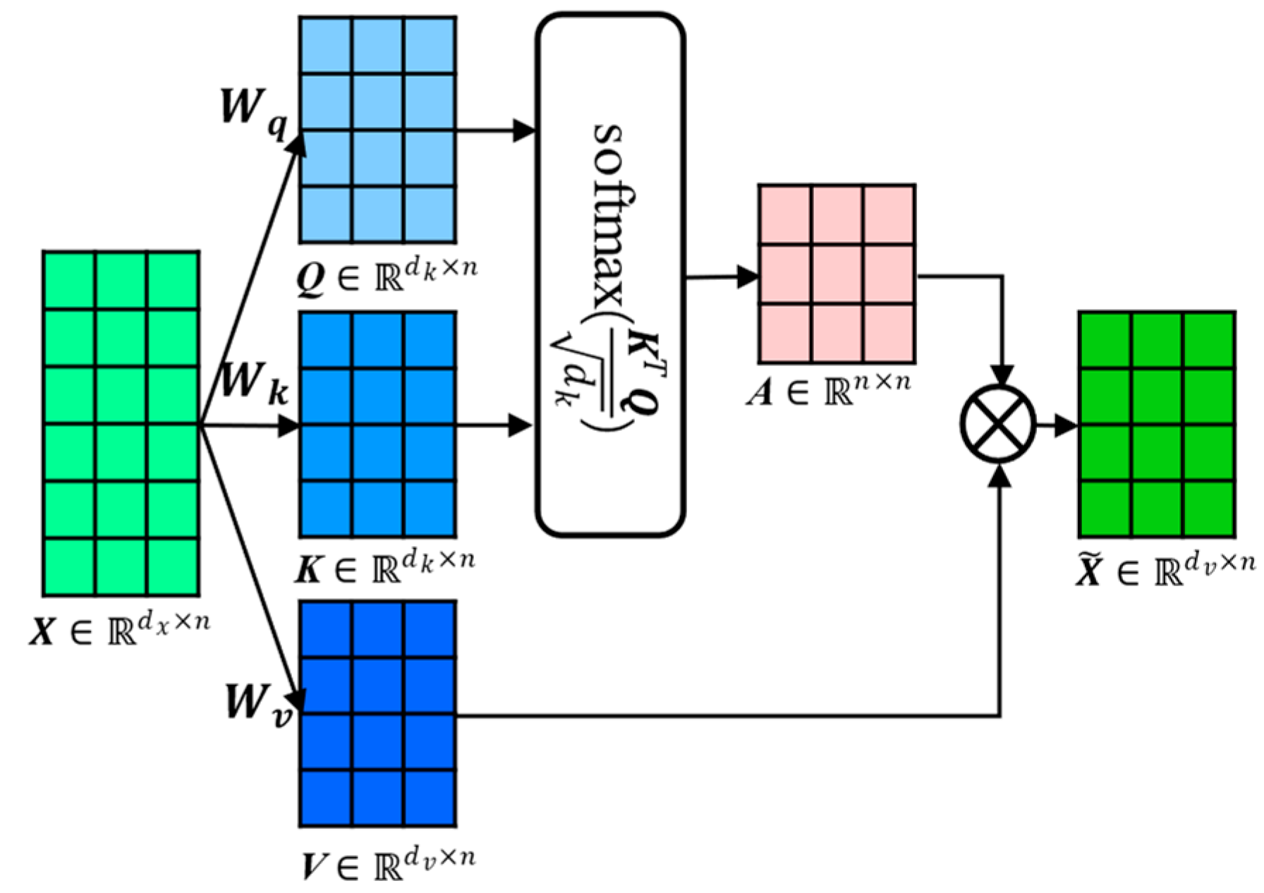
Different from the Bahdanau attention mechanism, self-attention [34], introduced in this study, not only allows the inputs to be focused on while producing outputs, but also enables the inputs to interact with one another (i.e., to compute the attention of all the other inputs with a single input). As seen in Figure 3, the precise mathematical processes of self-attention can be outlined as follows:

(1)

Given the multivariate input sequence $\mathit{X}{=[\mathit{x}}_1{,\dots ,\mathit{x}}_N]\in {\mathbb{R}}^{d_x\times n}$, denote the output sequence as $\tilde{\mathit{X}}{=[\tilde{\mathit{x}}}_1{,\dots ,\tilde{\mathit{x}}}_N]\in {\mathbb{R}}^{d_v\times n}$. Then, the key matrices $\mathit{K}$, the query matrices $\mathbf{Q}$, and the value matrices $\mathit{V}$, which consist of key vectors, query vectors, and value vectors, can be calculated using Equations (5)–(7), respectively.

$$\mathbf{Q}={\mathit{W}}_q\mathit{X}$$

(5)

$$\mathit{K}={\mathit{W}}_k\mathit{X}$$

(6)

$$\mathit{V}={\mathit{W}}_v\mathit{X}$$

(7)

where ${\mathit{W}}_q\in R^{d_k\times d_x}$, ${\mathit{W}}_k\in R^{d_k\times d_x}$, and ${\mathit{W}}_v\in R^{d_v\times d_x}$ are the parameter matrices, which are learned during the training process.

(2)

Choose a scaled dot-product as the attention score function, and calculate the score based on $\mathbf{Q}$, $\mathit{K}$.

(3)

Divide the score by the scaling factor (i.e., the square root of the key vector’s dimensions (d_k)), apply the softmax function to each self-attention attention score, and then multiply the score by $\mathit{V}$, as presented in Equation (8).

$$\tilde{\mathit{X}}=\mathit{V}\mathit{A}=\mathit{V}\mathrm{s}\mathrm{o}\mathrm{f}\mathrm{t}\mathrm{m}\mathrm{a}\mathrm{x}\left(\frac{{\mathit{K}}^T\mathit{Q}}{\sqrt{d_k}}\right)\in {\mathbb{R}}^{d_v\times n}$$

(8)

where $\mathit{A}$ represents the attention matrix and softmax is the normalization function.

3.2.2. Gated Recurrent Unit

Recurrent neural networks (RNNs) are a class of neural networks with a short-term memory capability that are used to handle sequential data, whose parameters can be learned using the backpropagation through time (BPTT) [39] algorithm. However, when the input sequence is relatively long, there are vanishing or exploding gradients; this is also known as the long-term dependencies problem [40].

Many approaches have been proposed to address the problem of long-term dependency. One of the earliest was to introduce a gating mechanism that supports the gating of the hidden state. This means using specific processes to determine when to recall and when to disregard information in the hidden state.

Among the many variants of RNNs, long short-term memory (LSTM) networks and gated recurrent unit (GRU) networks can effectively solve the vanishing and exploding gradient problem, and sufficiently mine the temporal characteristics and nonlinear features inherent in massive time-series data, so as to possess long-term memory effects and deep learning capabilities [41,42]. Compared with LSTM, GRU is a slightly more streamlined alternative that frequently provides comparable performance and is computed much more quickly [43,44].

The internal structure of a gated recurrent unit is shown in Figure 4. Let us assume that the input ${\mathit{X}}_t$ is a minibatch for a particular time step t, and the hidden state of the previous time step is ${\mathit{H}}_{t-1}$. Then, the reset gate ${\mathit{R}}_t,$ update gate ${\mathit{Z}}_t,$ candidate hidden state ${\tilde{\mathit{H}}}_t$, and the new hidden state ${\mathit{H}}_t$ are computed as follows:

$${\mathit{R}}_t=\sigma ({\mathit{X}}_t{\mathit{W}}_{xr}+{\mathit{H}}_{t-1}{W}_{hr}+{\mathit{b}}_r)$$

(9)

$${\mathit{Z}}_t=\sigma ({\mathit{X}}_t{\mathit{W}}_{xz}+{\mathit{H}}_{t-1}{\mathit{W}}_{hz}+{\mathit{b}}_z)$$

(10)

$${\tilde{\mathit{H}}}_t=\mathrm{t}\mathrm{a}\mathrm{n}\mathrm{h}({\mathit{X}}_t{\mathit{W}}_{xh}+({\mathit{R}}_t\odot {\mathit{H}}_{t-1}){\mathit{W}}_{hh}+{\mathit{b}}_h)$$

(11)

$${\mathit{H}}_t={\mathit{Z}}_t\odot {\mathit{H}}_{t-1}+\left(1-{\mathit{Z}}_t\right)\odot {\tilde{\mathit{H}}}_t$$

(12)

where ${\mathit{W}}_{xr},{\mathit{W}}_{xz}$, ${\mathit{W}}_{xh}$, ${\mathit{W}}_{hr}$, ${\mathit{W}}_{hz}$, and ${\mathit{W}}_{hh}$ are weight parameters; ${\mathit{b}}_r,{\mathit{b}}_z$, and ${\mathit{b}}_h$ are biases; $d$ represents the number of inputs; $n$ is the number of examples; $h$ is the number of hidden units; $\sigma$ is a sigmoid function; and the Hadamard (elementwise) product operator is represented by the symbol $\odot$.

3.3. Evaluation Metrics

To validate the effectiveness and superiority of the SAGRU model performance, three commonly used metrics, mean absolute error (MAE), root mean square error (RMSE), and determination coefficient (R²), were adopted in this study, which can be calculated using Equations (13)–(15).

$$RMSE=\sqrt{\frac{1}{N}\sum _{i=1}^N{\left(x_i-x_i^{\prime }\right)}^2}$$

(13)

$$MAE=\frac{1}{N}\sum _{i=1}^N|x_i-x_i^{\prime }|$$

(14)

$$R^2=1-\frac{\sum _{i=1}^N{\left(x_i-x_i^{\prime }\right)}^2}{\sum _{i=1}^N{(x_i-{\overline{x}}_i)}^2}$$

(15)

where $x_i$ is the “ith” measurement value, $x_i^{\prime }$ is the “ith” prediction value, and ${\overline{x}}_i$ is the mean of the total measurements.

4. Anomaly Detection Strategies

Based on historical healthy SCADA data and the proposed SAGRU network, the normal behavior model for critical components (e.g., main bearings, gearbox, generator) or subsystems (e.g., pitch system) of wind turbines can be established offline to learn the dynamic characteristics when operating under normal conditions, and then the early fault detection can be further captured through implementing the real-time condition monitoring.

Specifically, based on the well-trained SAGRU model, for offline testing datasets or online operating SCADA data, the residual values would be smaller with stable fluctuations when the wind turbine is operating under normal conditions. In abnormal conditions, the SAGRU model would produce larger residual values with violent fluctuations.

Therefore, as an indicator reflecting whether the wind turbine is in a normal or abnormal status, the prediction residual can be monitored in real time and statistically analyzed to identify deterioration conditions and detect potential faults.

Consequently, a hybrid anomaly detection approach consisting of change-point detection and a threshold alarm was proposed for wind turbine condition monitoring (WTCM) in this study; the detailed theory of the hybrid method is described in Section 4.1 and Section 4.2. Generally, a fault warning is triggered when detecting the change-points in the predicted residual sequence, which means that critical components are in deteriorated conditions and need to be paid attention to. Then, a fault alarm is triggered when the predicted residual exceeds the alarm threshold, which means that the deteriorated critical components have worsened further and may ultimately lead to wind turbine fault shutdown, and urgent maintenance measures need to be taken.

4.1. Alarm Threshold

As a nonparametric estimation method, the kernel density estimation (KDE) method was employed to calculate the probability density function (PDF) of the predicted residual when wind turbines are working normally to determine the alarm threshold. The detailed calculation steps are as follows.

Based on the KDE method and test dataset, the PDF of the residual can be computed according to Equation (16).

$$f\left(r\right)=\frac{1}{Nh}{\sum }_{i=1}^{N}K(\frac{r-r_i}{h})$$

(16)

where N represents the overall sample count, h is the smoothing parameter, and $K(·)$ represents the kernel function. Additionally, the Gaussian kernel function, shown in Equation (17), was selected for this study.

$$K(\frac{r-r_i}{h})=\frac{1}{h\sqrt{2\pi }}{\mathrm{e}}^{-\frac{(r-r_i{)}^2}{{2h}^2}}$$

(17)

According to the PDF calculated in step 1, the alarm threshold can be determined using Equation (18) for a given confidence $\alpha$. In this study, we chose $\alpha =99.7\%$ according to the three-sigma rule (3σ rule).

$$\alpha =P\left(r<r^{*}\right)={\int }_0^{r^{*}}f\left(r\right)dr$$

(18)

For online SCADA data, through applying condition monitoring, potential faults can be captured when the prediction residual continuously exceeds the alarm threshold.

4.2. Change-Point Detection

4.2.1. Change-Point Detection

The change-point detection algorithm (CPD) [45], first proposed in 1954 [46], is applied to find the change points in a univariate or multivariate time series. There is significant activity in the fields of statistics and signal processing using CPD, as well as a number of application contexts, including speech processing, financial analysis, bioinformatics, climatology, network traffic data analysis, and monitoring of complex systems.

Mathematically, for a given time series $y={\left\{y_t\right\}}_{t=t_1}^{t_T}$, which is split into K + 1 subsequences by the changepoint set $\mathcal{T}={\left\{t_1,t_2,\cdots ,t_K\right\}}_{K\le T}$, the aim of a change-point detection algorithm is to find the optimal changepoints set $\widehat{\mathcal{T}}$ corresponding to the best partitions $\widehat{\mathrm{P}}$ by minimizing the quantitative criterion $V\left(\mathcal{T},y\right)$ according to Equations (19) and (20).

(1)

For a univariate timeseries:

$$V\left(\mathcal{T},y\right)={\sum }_{k=1}^{K}C\left(y_{t_k:t_{k+1}}\right)$$

(19)

(2)

For a multivariate timeseries:

$$V\left(\mathcal{T},y\right)={\sum }_{d=1}^D{\sum }_{k=1}^{K}C\left(y_{t_k:t_{k+1}}^d\right)$$

(20)

where D represents the dimension of the time series, K is the number of changepoints, T is the length of the time series, $y_{t_k:t_{k+1}}$ represents a subsequence of time series, and C(·) represents the cost function.

It should be noted that, the number of change-points K can be set in advance or undetermined. Therefore, since K is set beforehand, the optimization issue investigated this research can be described as follows:

$$\underset{\left|\mathcal{T}\right|=K}{\min }V\left(\mathcal{T},y\right)$$

(21)

For an undetermined K, a constraint penalty term $pen\left(\mathcal{T}\right)$ should be added to restrict the number of detected changepoints.

$$\underset{\mathcal{T}}{\min }\tilde{V}\left(\mathcal{T},y\right)=\underset{\mathcal{T}}{\min }V\left(\mathcal{T},y\right)+pen\left(\mathcal{T}\right)$$

(22)

In summary, a changepoint detection algorithm generally comprises three basic components: a search method to look for $\mathcal{T}$, a cost function C(·), and a penalty term $pen\left(\mathcal{T}\right)$ when $K$ is undetermined.

4.2.2. Binary Segmentation Changepoint Detection

As a greedy sequential algorithm, a binary segmentation algorithm [35], denoted as BinSeg, is a well-known alternative to optimum approaches due to its straightforward conceptualization and straightforward implementation [36].

For timeseries $y$, the first changepoint calculation ${\widehat{t}}^{\left(1\right)}$ is computed using Equation (23).

$${\widehat{t}}^{\left(1\right)}=\underset{1\le t<T-1}{\mathrm{a}\mathrm{r}\mathrm{g}\mathrm{m}\mathrm{i}\mathrm{n}}V\left(\mathcal{T}=\left\{t\right\}\right)=\underset{1\le t<T-1}{\mathrm{a}\mathrm{r}\mathrm{g}\mathrm{m}\mathrm{i}\mathrm{n}}C\left(y_{0..t}\right)+C\left(y_{t..T}\right)$$

(23)

At ${\widehat{t}}^{\left(1\right)}$, the signal is split in half, and the same process is then carried out repeatedly on each of the resulting sub-signals until a stopping requirement is satisfied. Furthermore, this procedure is “greedy” in that it looks for the change points that will minimize the total cost the most. Hence, motivated by its low complexity, we adopt BinSeg as the search algorithm of the change-point detection method proposed in our study.

As for the cost function, the least squared deviation (denoted as CostL2) was employed in this study, which measures the mean shifts in a time series as written in Equation (24).

$$C\left(y_{\mathit{I}}\right)=\sum _{\mathrm{i}\in \mathit{I}}{\Vert y_{\mathrm{i}}-\overline{y}\Vert }^2$$

(24)

where $y_{\mathit{I}}$ represents the subsequence set and $\overline{y}$ is the mean of subsequence $y_{\mathrm{i}}$.

5. Case Study

In order to validate the practicability and effectiveness of the designed SAGRU–BinSegCPD method in actual application of wind turbine condition monitoring (WTCM), actual fault cases of main bearings were studied only using SCADA data, and the experimental results, comparative analysis, and a brief conclusion are presented in this section.

5.1. Dataset Description

The SCADA data utilized in this study were collected from multiple wind turbines on a wind farm situated in southern China, which consist of 33 wind turbines (EN-70/1.5) with a rated power of 1500 kW. The records from the SCADA system were sampled every 10 min, and every record includes nearly 100 discrete pieces of information as well as 32 continuous parameters as displayed in

Table 1. Continuous status parameters in SCADA system.

Continuous Parameters
Wind direction	Ambient temperature	Generator speed	Reactive power
Wind speed	Hub temperature	Generator front bearing temperature	Power factor
Blade 1 angle	Nacelle temperature	Generator rear bearing temperature	Current phase L1
Blade 2 angle	Main shaft speed	Generator stator winding U temperature	Current phase L2
Blade 3 angle	Main bearing temperature	Generator stator winding V temperature	Current phase L3
Blade 1 motor temperature	Gearbox front bearing temperature	Generator stator winding W temperature	Voltage phase L1
Blade 2 motor temperature	Gearbox rear bearing temperature	Actual torque	Voltage phase L2
Blade 3 motor temperature	Gearbox oil temperature	Active power	Voltage phase L3

.

In this paper, 155,818 data records collected from five wind turbines were studied during the periods of 1 January 2019–31 December 2019, 1 April 2020–9 April 2020, 9 August 2020–16 August 2020, and 22 August 2020–23 August 2020, among which 153,567 data samples were used to construct the normal behavior model of the main bearings, 1166 data samples for the normal condition monitoring validation, and 1085 data samples for the abnormal condition monitoring validation. The detailed dataset description is shown in

Table 2. Description of dataset used for modeling.

Dataset	Name of Wind Turbine	Time Range (dd/mm/yyyy)	Fault Time	Fault Mode	Number of Raw Data	Number of Valid Data
Modeling dataset A for training, validation, and testing	A09, A12, A16	1 January 2019–31 December 2019	/	/	153,567	125,080
Dataset B1 for normal condition monitoring	A20	1 April 2020–9 April 2020	/	/	1166	/
Dataset B2 for abnormal condition monitoring	A17	9 August 2020–16 August 2020	15:38 16 August 2020	Main bearing overtemperature	1085	/
		22 August 2020–23 August 2020

.

As can be seen from Table 2, WTs A09, A12, A16, and A20 operated under normal conditions during the studied time periods, whereas WT A17 suffered from main bearing over-temperature fault at 15:38 on 16 August 2020. Before being utilized to build the condition monitoring model for the main bearings, the raw SCADA data of WTs A09, A12, and A16 should be subjected to data cleaning to obtain a health dataset. Additionally, 125,080 normal data samples were reserved and split into three sub-datasets (i.e., A1, A2, and A3) in a ratio of 0.8:0.1:0.1, one for model training, one for model validation, and the other for model testing, respectively. Meanwhile, all three datasets A, B1, and B2 also need to be normalized prior to modeling.

Considering the model performance and computing efficiency, it was necessary to implement variable selection based on the $R_s$ calculated using Equation (4) to remove variables with lower correlation coefficients and reserving variables with higher correlation coefficients. The partial Spearman correlation coefficient (SCC) calculation results for the variable selection is presented in

Table 3. Result of Spearman correlation coefficients (SCCs).

No	Variable	Unit	|Rs|	No	Variable	Unit	|Rs|
1	Hub temperature	°C	0.7490	9	Generator front bearing temperature	°C	0.4997
2	Ambient temperature	°C	0.6951	10	Gearbox oil temperature	°C	0.4708
3	Control cabinet temperature	°C	0.6649	11	Gearbox front bearing temperature	°C	0.4559
4	Gearbox inlet oil temperature	°C	0.5542	12	Wind speed	m/s	0.3703
5	Generator rear bearing temperature	°C	0.5343	13	Gearbox rear bearing temperature	°C	0.3681
6	Nacelle temperature	°C	0.5305	14	Main shaft speed	rpm	0.3634
7	Blade 1 motor temperature	°C	0.5200	15	Generator speed	rpm	0.3632
8	Active power	kW	0.5105	16	Generator stator winding U temperature	°C	0.3376

.

As displayed in Table 3, 16 variables, including ambient temperature, hub temperature, nacelle temperature, and active power, were selected as model inputs, while the main bearing temperature was used as the model output.

5.2. Model Validation

After the data preprocessing and variable selection, using the three sub-datasets (i.e., A1, A2, and A3) described in Section 5.1, the SAGRU normal behavior model for the main bearings for condition monitoring was established and trained. Meanwhile, to validate the practicability and superiority of the constructed SAGRU model, five other models, including conventional algorithms (e.g., XGBoost and BPNN), standard recurrent neural networks (e.g., RNN and GRU), and attention recurrent neural networks (e.g., feature-attention GRU, denoted as FAGRU, and time attention GRU, denoted as TAGRU), were used for comparison.

The number of estimators and the learning rate of XGBoost were set to 100 and 0.1, respectively. The structure of the BPNN model was designed as 16-32-16-8-1. Additionally, the hyperparameters of the rest of the RNN (i.e., RNN, GRU, FAGRU, TAGRU, and SAGRU) models were set to identical values for comparison, which are displayed in

Table 4. Hyperparameters of RNNs.

Hyper-Parameters	Algorithms/Values	Hyper-Parameters	Algorithms/Values
Loss function	MSE	Number of steps	8
Optimization algorithm	Adam	Number of epochs	1000
Batch size	64	Learning rate	0.001

.

Next, the constructed SAGRU model and six other models (i.e., XGBoost, BPNN, RNN, GRU, FAGRU, and TAGRU) were trained, validated, and tested. Additionally, for the test sub-dataset A3, the quantitative evaluation metrics of the prediction results from all models were calculated, which are listed in

Table 5. Evaluation results of different models.

Model	MAE (°C)	RMSE (°C)	R2	Model	MAE (°C)	RMSE (°C)	R2
XGBoost	0.7363	1.1587	0.7861	TAGRU	0.4219	0.6485	0.8906
BPNN	0.756	1.0602	0.8129	FAGRU	0.4072	0.6434	0.8995
RNN	0.628	0.8724	0.8572	SAGRU	0.3048	0.4937	0.9203
GRU	0.4941	0.7683	0.878	Mean of AMGRUs	0.3779	0.5953	0.9035

.

It can be clearly observed from Table 5 that, compared with non-RNN models (i.e., XGBoost and BPNN), RNN models had better forecasting performances and lower RMSEs and MSEs, and a higher R². This is mainly because RNNs are a class of neural networks with short-term memory capabilities that are used to handle sequential data and can mine the temporal features inherent in the SCADA time series. Thus, RNN models can better learn the normal behaviors of the temperature of the main bearings.

Additionally, from Table 5, we can also discover that, in terms of three metrics (i.e., MSE, RMSE, and R²), the GRU model performed better than the RNN model. The primary factor is that, by the introduction of a gated mechanism, GRU can solve the vanishing or exploding gradients problem that exists in RNNs when the input sequence is relatively long, thereby improving the model performance to a certain extent.

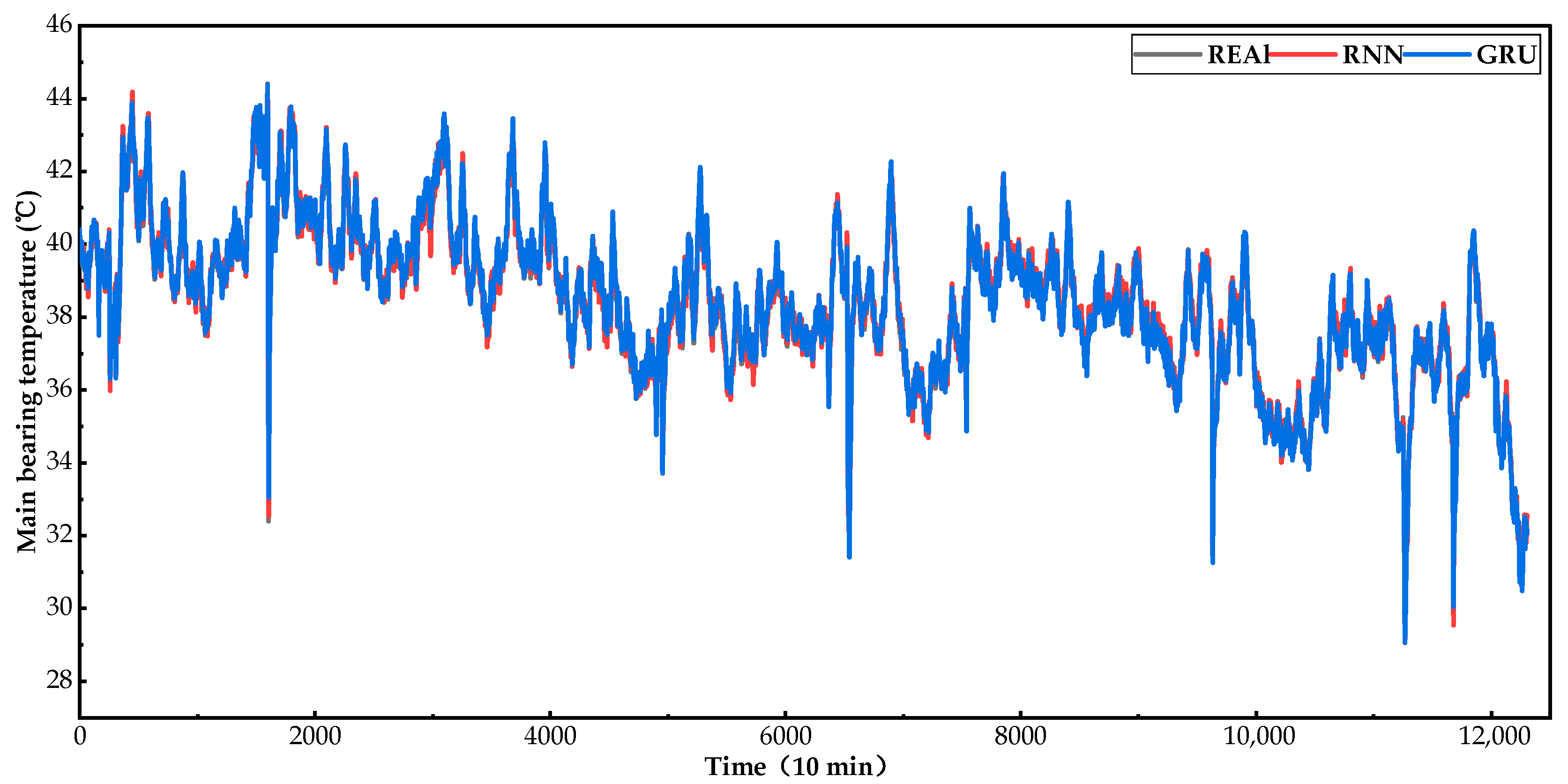
The curves displayed in Figure 5 and Figure 6, intuitively display the prediction results of main bearing temperatures for the test sub-dataset A3 using an RNN and GRU. As can be observed in Figure 5 and Figure 6, both models were able to capture the normal behavior of the main bearings, but GRU was superior to the RNN.

As described in Section 3.2.1, an attention mechanism (AM) can optimize resource allocation and enable RNN models to concentrate on the input variables that are more critical and highly correlated with the output variable, thus further improving the prediction accuracy of RNN models. Therefore, through introducing three attention mechanisms (i.e., feature attention, time attention, and self-attention), we can further achieve a performance improvement for the GRU model.

As indicated from the quantitative evaluation results in Table 5, the AMGRUs (i.e., FAGRU, TAGRU, and SAGRU) generally gave a higher modeling precision. In terms of RMSE and MSE, the average values of the AMGRUs were 0. 3779 °C and 0. 5953 °C, which were 23.51% and 22.53% lower than that of GRU, respectively. Additionally, the mean R² of the AMGRUs was 0.9035, which was 2.55% higher than that of GRU.

It can be also found from Table 5 that, compared with the other two attention mechanisms, the self-attention mechanism produced the maximum performance improvement for GRU from the following three aspects: RMSE, MSE, and R². The MSE and RMSE of SAGRU were 0. 3048 °C and 0. 4937 °C, which were 38.3% and 35.7% lower than those of GRU, and the R² of SAGRU as 0.9203, which was 4.23% higher than that of GRU. In other words, among the three AMGRU models, the constructed SAGRU model had the best prediction performance due to having the lowest RMSE and MSE, and highest R².

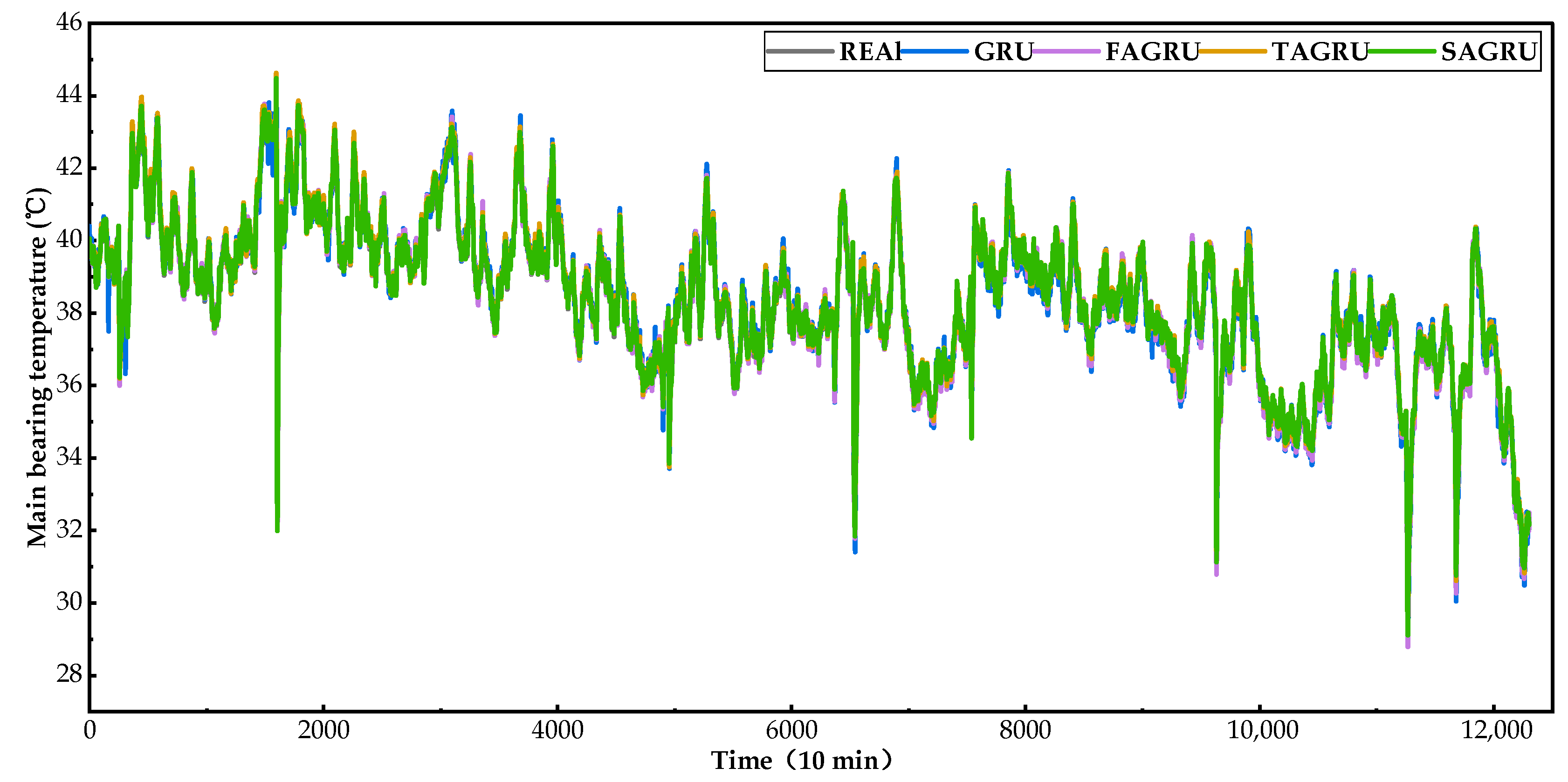
Meanwhile, as presented in Figure 7 and Figure 8, the prediction results of SAGRU were closer to the practical main bearing temperature in the comparison with FAGRU and TAGRU. Thus, from Figure 7 and Figure 8, a similar conclusion that SAGRU can better track the dynamic changing trend of the main bearings can be drawn, corresponding to the results in Table 5. This is mainly because the proposed SAGRU model can better mine the nonlinear dynamic temporal features inherent in the SCADA data and learn the normal behaviors of the main bearings by introducing a self-attention mechanism. Hence, it is feasible and promising to establish the SAGRU model for potential fault detection of wind turbine main bearings.

Consequently, according to the above evaluation results and comparative analysis, in this study, the SAGRU network was employed to construct a normal behavior model of main bearings for condition monitoring.

5.3. Normal Condition Monitoring

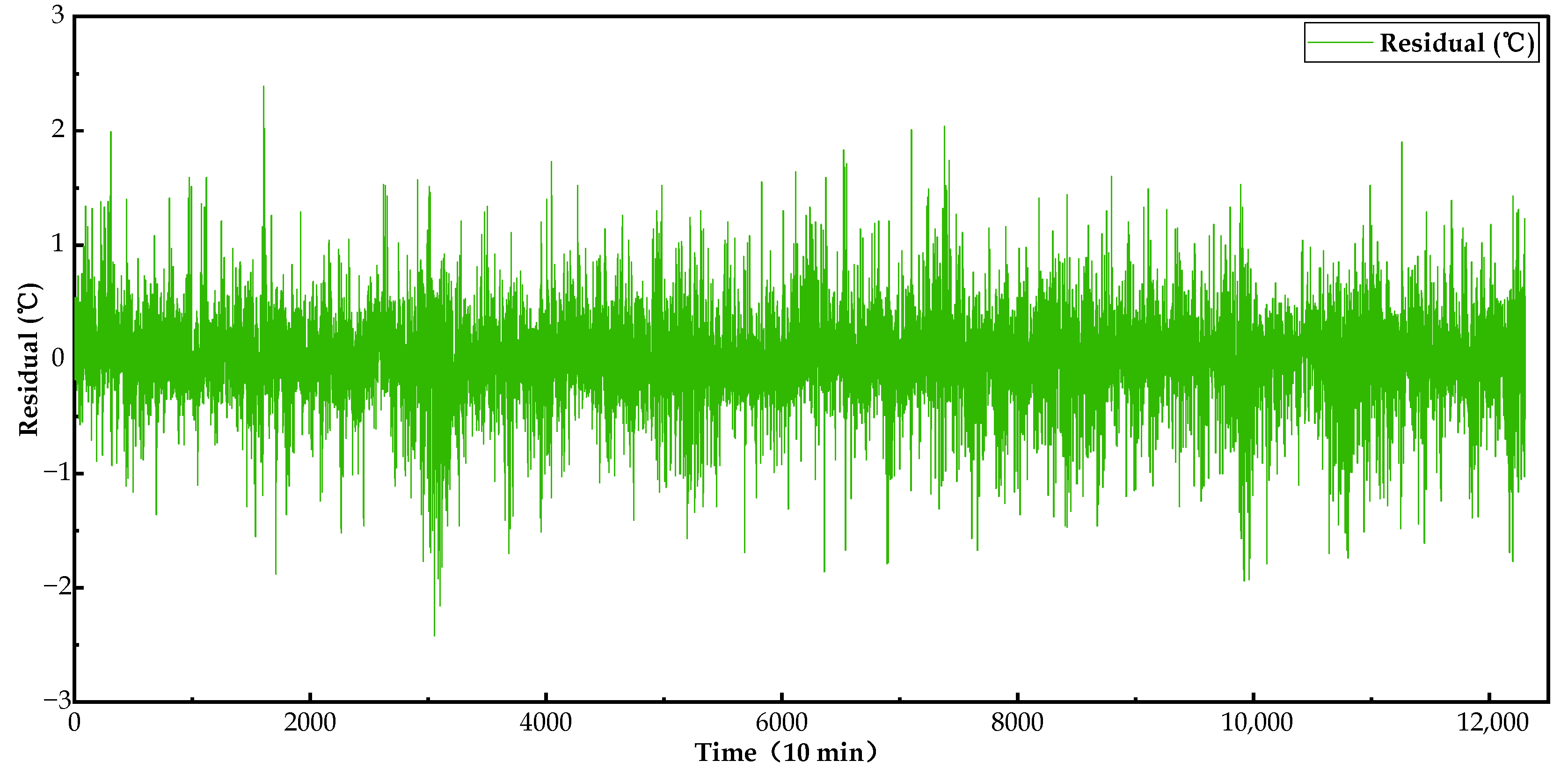
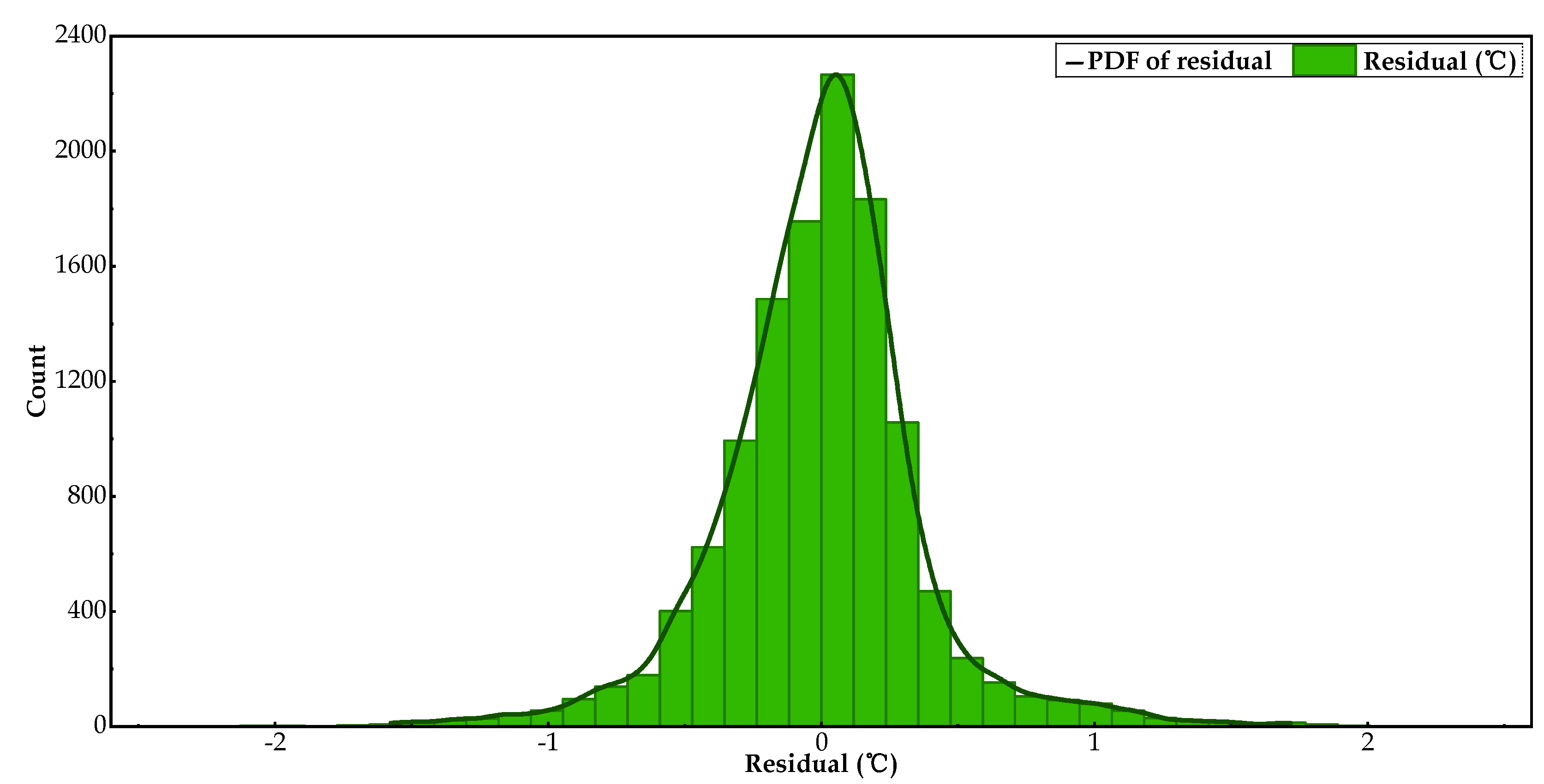
Based on the well-trained SAGRU model and the test sub-dataset A3, the residuals between the measurements and the predictive values of the main bearing temperature when the wind turbine is operating under normal conditions was obtained, which is shown in Figure 9. Next, according to the KDE algorithm described in Section 4.1, the PDF of the predicted residuals was estimated using Equation (16) and is presented in Figure 10. Additionally, for a given confidence $\alpha =99.7\%$ set using the three-sigma rule (3σ rule), the alarm threshold was calculated as 2.03 °C using Equations (17) and (18).

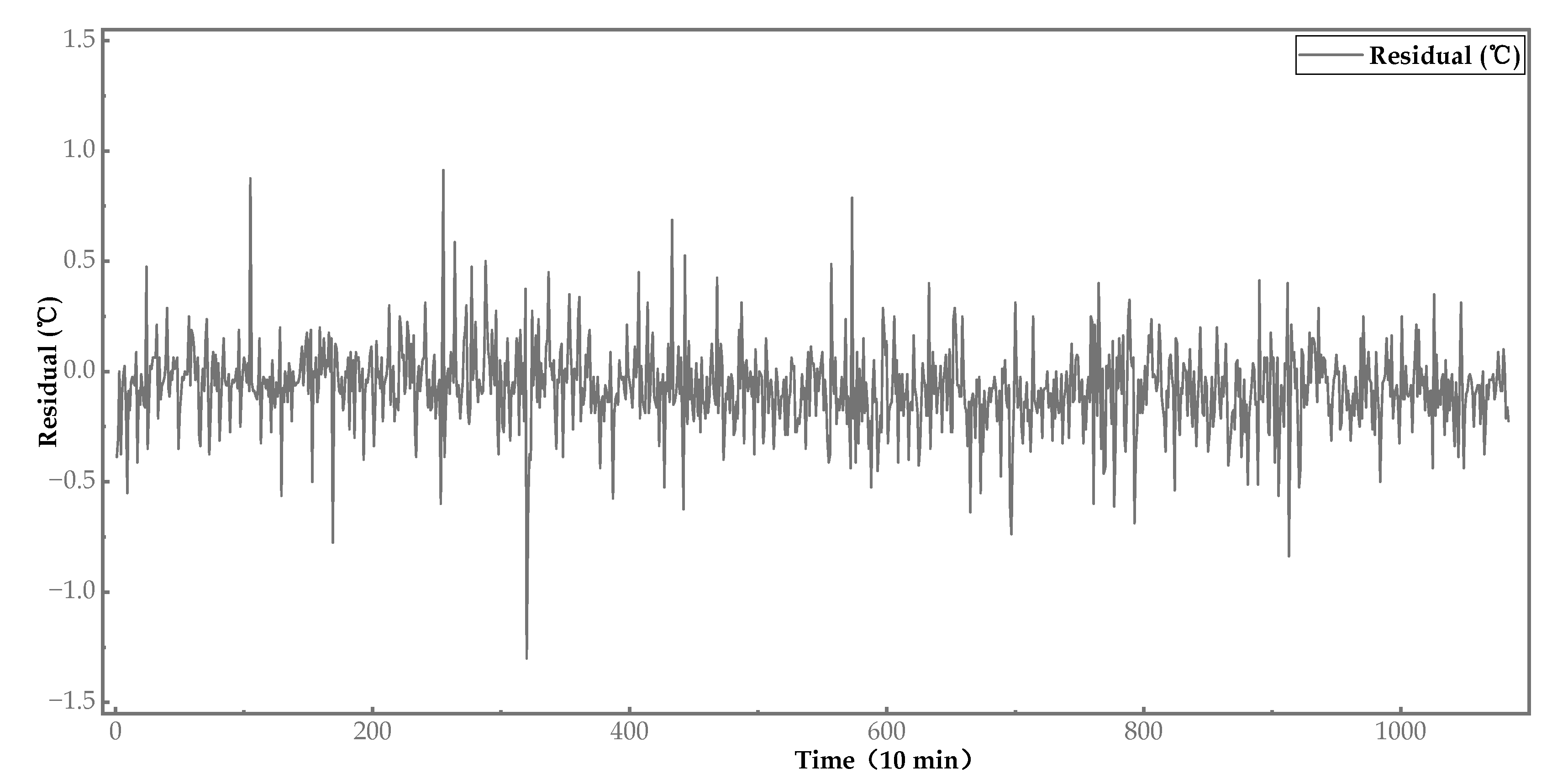
According to the operation and maintenance (O&M) records, during the period of 1 Apirl 2020–9 Apirl 2020, WT A20 operated under normal conditions and did not experience a main bearing fault. Therefore, dataset B1, the available historical SCADA data for WT A20, was gathered and preprocessed to test the capability of the proposed SAGRU for normal behavior condition monitoring, and the condition monitoring results are displayed in Figure 11. As seen in Figure 11, all residuals that indicated a difference between the measurements and prediction values of the main bearing temperature of WT A20 fell within the alarm threshold of 2.03 °C. Thus, it can be inferred that the constructed SAGRU model was able to precisely learn the normal behavior of the main bearings.

5.4. Abnormal Behavior Detection Validation

To further validate the effectiveness of the designed SAGRU–BinSegCPD method in identifying the abnormal behavior of the main bearings of wind turbine, WT A17 was used for investigation. According to the O&M records, WT A17 experienced a main bearing over-temperature fault at 15:38 on 16 August 2020 and restarted at 12:10 on 22 August 2020 after maintenance. Therefore, dataset B2, consisting of 1085 SCADA samples collected from two periods (i.e., 9 August 2020–16 August 2020 and 22 August 2020–23 August 2020) was utilized to verify the early fault warning capability of the designed method. Additionally, the detailed fault information of WT A17 is as follows.

A fault alarm message of main bearing over-temperature was issued by the SCADA system at 15:38 on 16 August 2020. Then, after receiving the alarm signal, the technicians of the wind farm immediately went to address the fault and found that the temperature sensor PT100 wire was loose. However, after tightening the wire, they found that the main bearing temperature was still fluctuating at higher values compared with the health reference values in normal conditions. Next, through endoscopic examination, they found that there was regional damage and extrusion marks on the outer raceway, inner raceway, and rollers of the main bearings. Therefore, it can be inferred that, during the operation of WT A17, the bearing damages caused by abnormal loads had accumulated over the measurement time period and became sufficiently severe so as to result in over-temperature fault in the main bearings. The endoscopic examination results of the roller, inner raceway, and outer raceway of the WT A17 main bearings are shown in Figure 12.

5.4.1. Threshold Alarm

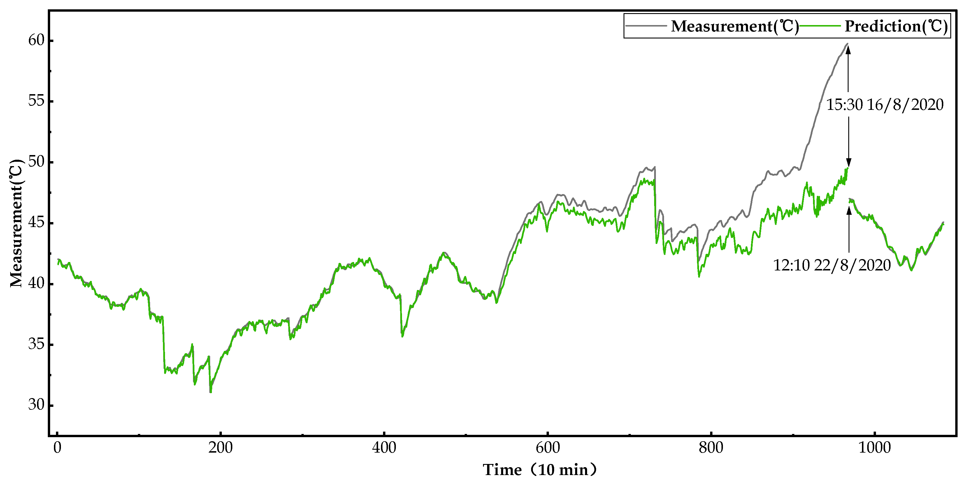
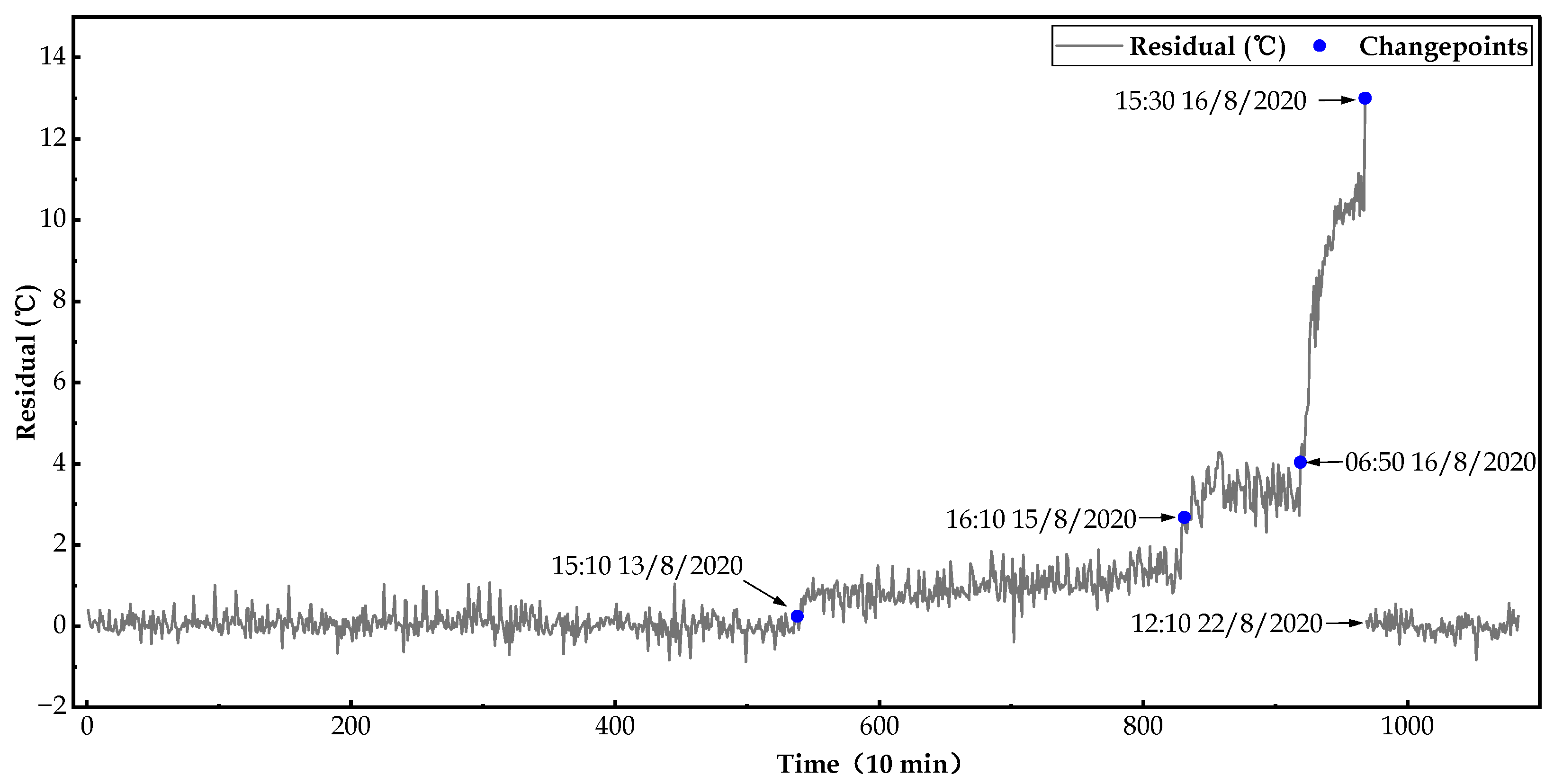
Based on the well-trained SAGRU model, the prediction results for the fault dataset B2 (WT A17) are shown in Figure 13. Additionally, according to the hybrid anomaly detection strategies (i.e., threshold alarm and change-point detection) described in Section 4, the fault detection results of WT A17 main bearings are displayed in Figure 14.

As found in Figure 13 and Figure 14, the predicted residual between the actual measurements and the predicted values fluctuated steadily around 0 before 14:50 on 13 August 2020, then started to increase generally until exceeding the alarm threshold 2.03 °C at 15:50 on 15 August 2020. Then, starting at 06:40 on 16 August 2020, the residual began to vibrate violently, and rose to the maximum value at 15:30 on 16 August 2020 corresponding to the time when the SCADA system issued a main bearing over-temperature signal. Consequently, it can be concluded that, compared with the actual failure time, the alarm threshold calculated in Section 5.3 can detect the main bearing over-temperature fault approximately 23.8 h in advance.

Nevertheless, the threshold alarm strategy has limitations in that a too large or small alarm threshold would result in missed alarms or false detections, respectively. Therefore, to address the limitations mentioned above and improve the timeliness and reliability of anomaly detection, a hybrid anomaly detection strategy was proposed for wind turbine condition monitoring. In other words, for the prediction residual sequence generated using the SAGRU model in this study, we not only used the alarm threshold to detect the potential faults of the main bearings, but also employed the BinSegCPD algorithm to automatically identify deterioration statuses of the main bearings.

5.4.2. Change-Point Detection

Based on the SAGRU model and the BinSegCPD algorithm described above, for the fault dataset B2 (WT A17), the change-point detection result of the prediction residual sequence is displayed in Figure 15. As can be concluded from Figure 15, there were altogether four changepoints in the prediction residual sequence, namely 15:10 13 August 2020, 16:10 15 August 2020, 06:50 16 August 2020, and 15:30 16 August 2020, which correspond to the deterioration states of the main bearings.

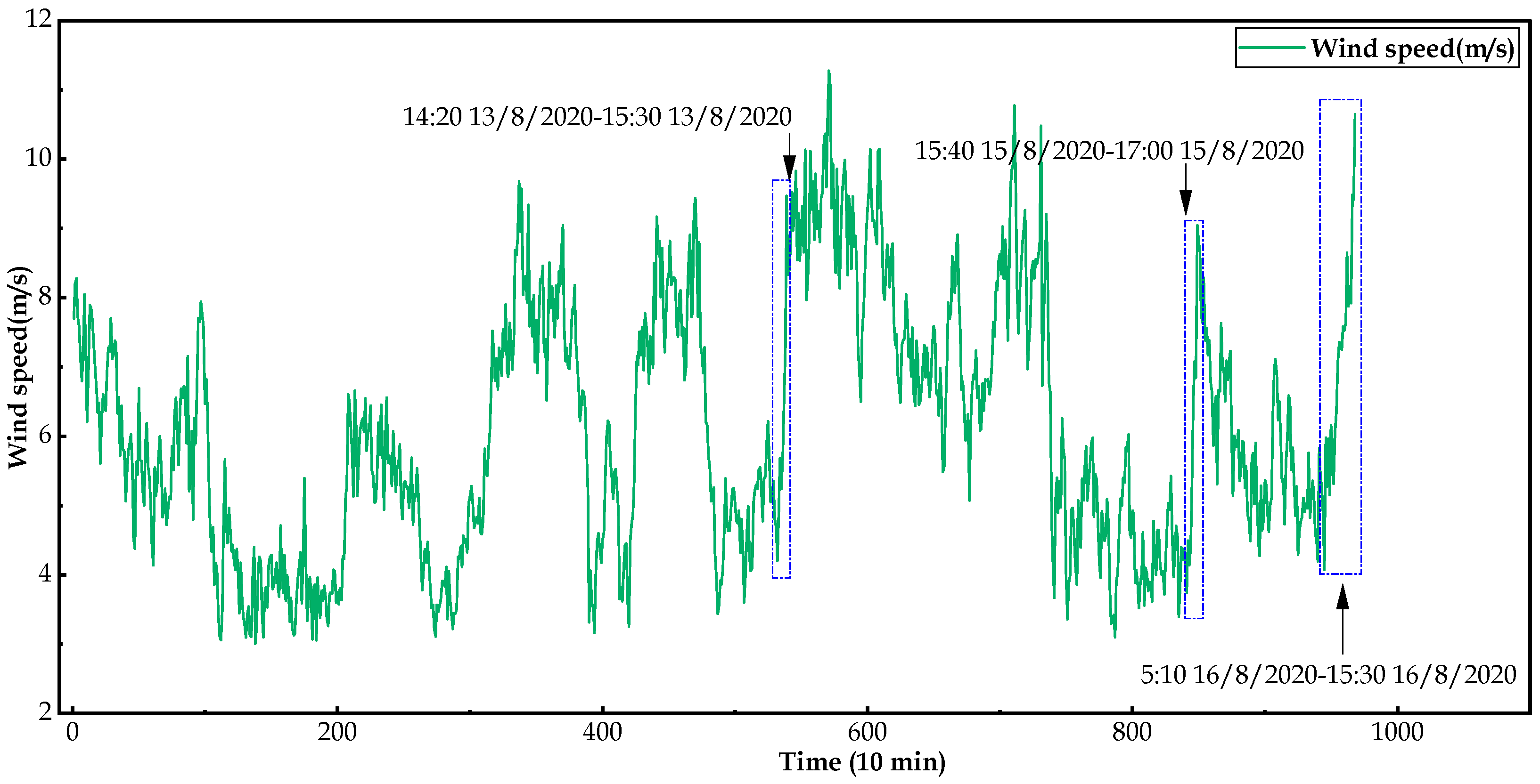
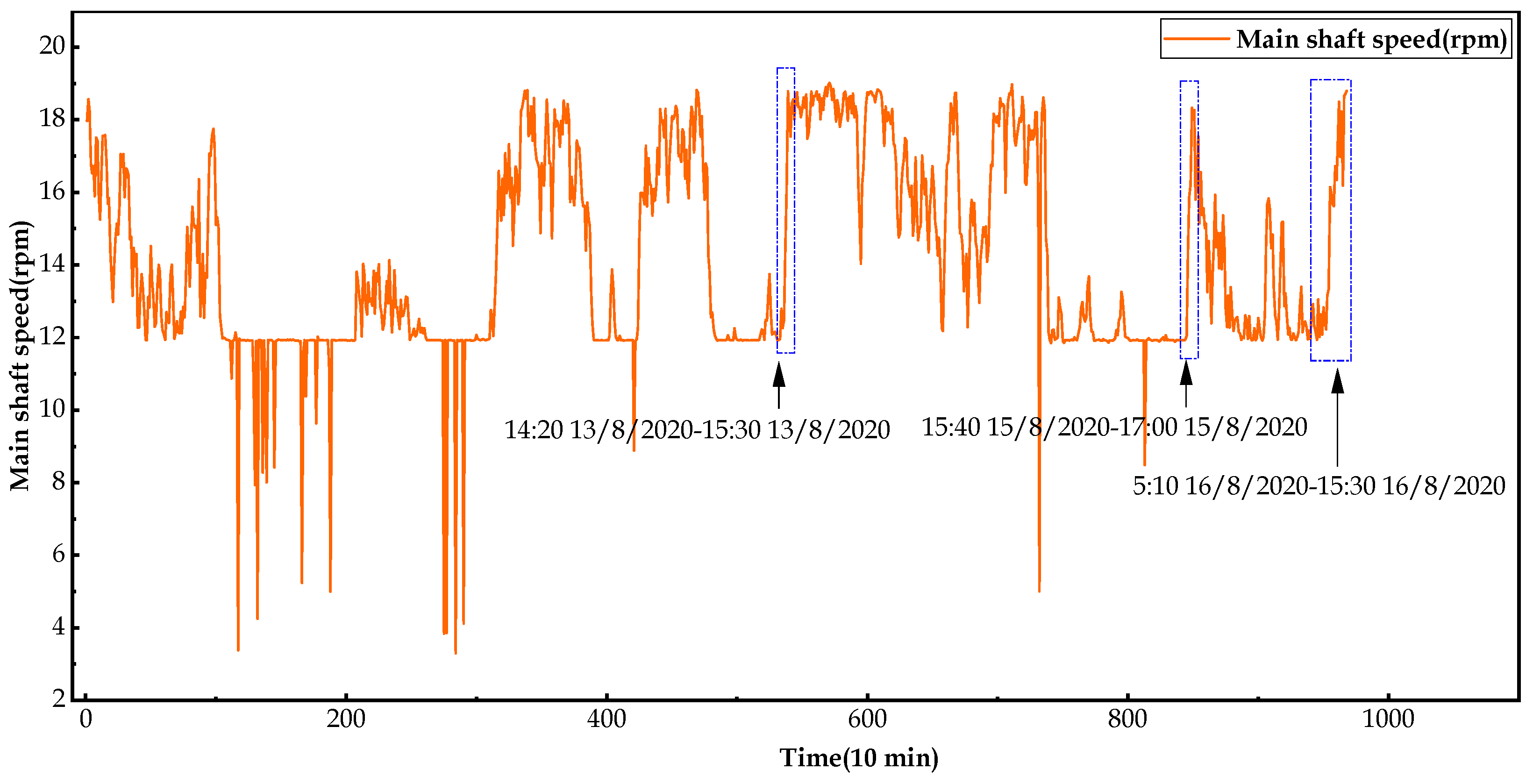
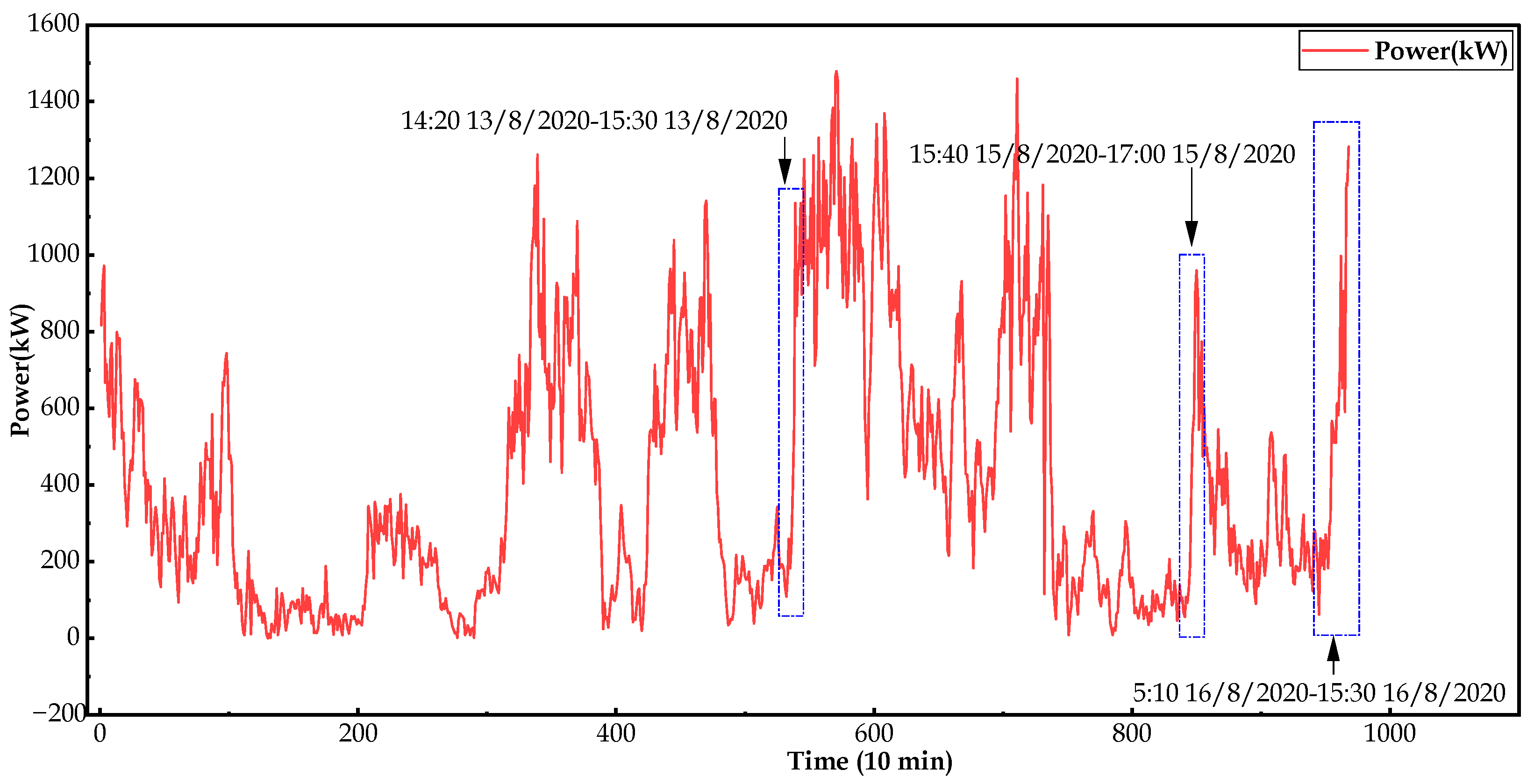
Additionally, Figure 16, Figure 17 and Figure 18 display the wind speed, main shaft speed, and active power of WT A17 during the fault period from 9 August 2020 to 16 August 2020.

Consequently, combined with the O&M logs, the conclusions can be drawn as follows. Starting at 15:10 on 13 August 2020 (i.e., change-point 1), it can be clearly observed that the main bearings had begun to suffer from mechanical damage, which may have been caused by violent wind changes in a short time. As can be observed in Figure 16, Figure 17 and Figure 18, the wind speed of WT A17 sharply climbed from 4.2 m/s to 9.47 m/s during the period 14:20 13 August 2020–15:30 13 August 2020, and the main shaft speed and power of WT A17 rapidly increased from 11.92 rpm to 18.79 rpm and from 109.41 kW to 1135.75 kW, respectively.

After long-term operation with potential mechanical damage, the main bearing gradually deteriorated and the prediction residual of the SAGRU model started to increase correspondingly. Around 16:10 on 15 August 2020 (i.e., change-point 2), the residual further significantly increased, which indicates more severe damage for the WT A17 main bearings. Figure 16, Figure 17 and Figure 18, during the period 15:40 15 August 2020–17:00 15 August 2020, indicate that another wind rapid change, rapidly rising from 3.74 m/s to 9.04 m/s, may have resulted in the above residual fluctuations.

Meanwhile, change-points 3 and 4 were detected in the period of 5:10 16 August 2020–15:30 16 August 2020, during which the predicted residual sharply rose to 13.01 °C, as shown in Figure 14, and the wind speed, main shaft speed, and power of WT A17 quickly increased from 4.08 m/s to 10.64 m/s, from 11.93 rpm to 18.80 rpm, and from 62.03 kW to 1282.58 kW, respectively, as shown in Figure 16, Figure 17 and Figure 18. Hence, the PT100 wire likely became loose around 06:50 on 16 August 2020 (i.e., change-point 3), whereas change-point 4 (15:30 16 August 2020) corresponds to the time point when the SCADA system issued an alarm signal at 15:38 on 16 August 2022.

In summary, compared with the actual failure time, the BinSegCPD algorithm could identify the deterioration conditions of the WT A17 main bearing 72.47 h in advance. Additionally, the proposed hybrid anomaly detection strategy (i.e., combining threshold alarm and changepoint detection) can not only improve the timeliness and reliability of anomaly detection, but also provide data and theoretical support for follow-up fault analysis.

6. Conclusions

In this study, based on a GRU network with a self-attention mechanism (SAGRU) and the binary segmentation changepoint detection algorithm (BinSegCPD), a novel condition monitoring approach for wind turbines was designed. Additionally, compared with five other models, the effectiveness, superiority, timeliness, and reliability of the proposed SAGRU–BinSegCPD method were fully validated using two years of SCADA data collected from multiple wind turbines.

On the one hand, a normal behavior model for wind turbines was established based on the SAGRU model, which can more effectively learn the sophisticated nonlinear correlations and temporal characteristics within different monitoring variables. Compared with the GRU model, the MSE and RMSE of SAGRU were 0. 3048 °C and 0. 4937 °C, which were 38.3% and 35.7% lower than those of GRU, and the R² of SAGRU was 0.9203, which was 4.23% higher than that of GRU. On the other hand, a hybrid anomaly detection strategy, combining a threshold alarm and changepoint detection, was introduced for wind turbine condition monitoring. The hybrid strategy can significantly improve the timeliness and reliability of wind turbine anomaly detection. Based on the fault dataset B2 and compared with the actual failure time, the experimental results demonstrated that the hybrid strategy automatically identified deterioration conditions in the main bearings 72.47 h in advance.

In future studies, we plan to employ intelligent optimization algorithms (e.g., sparrow search algorithm, particle swarm optimization algorithm, and crisscross optimization algorithm) to optimize the SAGRU hyperparameters to further enhance model performance. Additionally, the proposed condition monitoring method will be extended to a wider application, such as the generator, gearbox, and blade of wind turbines.