Article

Power Quality Disturbance Classification Based on Parallel Fusion of CNN and GRU

College of Physics and Optoelectronic Engineering, Shenzhen University, Shenzhen 518060, China
*
Author to whom correspondence should be addressed.
Energies 2023, 16(10), 4029; https://doi.org/10.3390/en16104029
Submission received: 11 April 2023 / Revised: 3 May 2023 / Accepted: 9 May 2023 / Published: 11 May 2023
(This article belongs to the Special Issue Analysis of Electricity Distribution Network and Electricity Markets)

Abstract

:
Effective identification of complex power quality disturbances (PQDs) is the premise and key to improving power quality issues in the current complex power grid environment. However, with the increasing application of solid-state switches, nonlinear devices, and multi-energy system generation, the power grid disturbance signals are distorted and complicated. This increases the difficulty of PQDs identification. To address this issue, this paper presents a novel method for power quality disturbance classification using a convolutional neural network (CNN) and gated recurrent unit (GRU). The CNN consists of convolutional blocks, some of which come with a squeeze-and-excitation block (SE), and is used to extract the short-term features from PQDs, where the convolutional block is used to capture the spatial information from PQDs and the SE is used to enhance the feature extraction capability of the convolutional neural network. The GRU network is designed to capture the long-term feature from PQDs, and an attention mechanism connected to GRU’s hidden states at different times is proposed to improve the GRU’s feature capture ability in long-term sequences. The CNN and GRU are parallelly arranged to perceive the same PQDs in two different views, and the feature information extracted from them is fused and transmitted to the Softmax activation layer for classification. Based on MATLAB-Simulink, a typical multi-energy-source system is constructed to analyze PQDs, and twelve PQDs are simulated to validate the proposed method. The simulation results show that the proposed method has higher classification accuracy in both single and hybrid disturbances and significant advantages in noise immunity.

1. Introduction

With the development of smart grids, the large-scale integration of advanced power electronic devices, electric vehicles, and multi-energy system have brought new challenges to the operation of distribution networks [1]. The high penetration level of renewable energies requires the use of operation and management strategies to maintain and enhance the reliability, efficiency, and safety of the power grid [2]. Fundamentally, the extensive use of power electronics equipment, combined with a tremendous number of nonlinear loads in the power system, has resulted in an increase in both single PQDs and compound PQDs. This situation poses enormous challenges to the power grid, ultimately affecting the reliability of power system operation [3]. Therefore, detecting and classifying PQDs accurately and efficiently is key to resolving power quality problems [4].
Traditionally, the classification of PQDs is divided into three stages: feature extraction, feature selection, and feature classification [5]. There are many methods based on signal processing for feature extraction and feature selection, such as short-time Fourier transform [6], wavelet transform [7], wavelet packet transform [8], S-transform [9], and Hilbert Huang transform [10]. All of these methods can extract spatial–temporal features of PQDs, enabling the identification of PQDs. Feature classification is responsible for associating the PQDs with selected feature types, and machine learning classifiers such as decision tree [11], support vector machine [12], Bayesian decision [13], artificial neural network (ANN) [14], and random forest [15] classifiers are commonly used for this purpose. It is important to recognize that the performance of the classifier is directly affected by the choice of features. However, there are still two issues that need to be addressed. The first issue is that the features extracted from PQDs are often artificially selected and heavily dependent on expert experience. The second issue is that the classifier may encounter difficulties in accurately classifying complex compound PQDs [16].
Deep learning is widely used in various fields such as image, signal, and information processing. In recent years, researchers have started exploring the application of deep learning to the classification of PQDs. One of the key advantages of a deep learning network is its ability to automatically select features, since it consists of both feature extraction and classifier components that update simultaneously during the learning process. This represents a significant improvement over traditional machine learning classifiers that typically rely on manually selected features. Garcia et al. [17] utilized a CNN [18] to classify PQDs. A CNN has a very efficient ability to obtain short-term information from PQDs. In [19], a multi-fusion convolutional neural network is utilized for the classification of PQDs with a focus on automatic extraction and fusion of features from multiple sources. It combines time and frequency domain information to enable the automatic classification of complex PQDs. As stated in [20], a sequence-to-sequence deep learning model based on the GRU [21] is proposed for the recognition of power quality disturbance types and their corresponding time locations. The model is capable of recognizing the type of each element in the sequence and subsequently locating the starting and ending times of the disturbances. Junior et al. [22] and Mohan et al. [23] utilized a CNN combined with long short-term memory in series (CNN-LSTM) to classify PQDs. The CNN-LSTM model applies a CNN to extract features and long short-term memory (LSTM) [24] to filter and update these features. By combining these layers, CNN-LSTM performs the automated extraction, selection, and classification of PQDs, unifying the problem into a single task. Kumar et al. [25] employed S-Transform, ANN, and rule-based decision trees to classify PQDs. S-matrix contours such as maximum amplitude versus time and amplitude versus frequency from the S-Transform matrix clearly depict the disturbance patterns of the power system. Feature extraction from the S-Transform was utilized to train the ANN. Decision rules were then used to map observations about an item to determine its target value, representing the decision-making process. This method effectively classifies both single and compound disturbances, with the S-Transform matrix clearly showing the disturbance modes of the power system. However, the feature acquisition and network training processes are separate, resulting in decreased network training efficiency and classification accuracy compared to deep learning networks that integrate both processes.
The application of deep learning in PQD problems can not only improve the classification accuracy, but also save manpower and simplify the processes. However, the methods mentioned above such as CNNs or recurrent neural networks (RNNs) may have some limitations. For example, although a CNN can improve its feature extraction ability through multilayer stacking, it may not be able to fully capture the temporal correlation of the feature information extracted from PQDs. Similarly, while an RNN can extract temporal features from time series data, it may be challenging to extract the full feature information from long time series data such as PQDs. Although the CNN-LSTM method combines the advantages of CNN and LSTM, the temporal feature extracted from CNN may not be comprehensive enough, which could affect the further improvement of classification accuracy.
Given the above difficulties, the main contributions of this paper are as follows:
(1)
This paper proposes a novel parallel constructional network (called CNN-GRU-P) composed of a CNN block and a GRU network block for classifying PQDs. By transmitting PQDs into both network blocks simultaneously, the proposed method provides a more comprehensive understanding of the PQDs from two different views. The output of the two networks is fused through the fully connected layer and then transmitted to the Softmax activation layer for classification to obtain a more accurate classification result.
(2)
A CNN is utilized to extract short-term features from input PQDs. To further improve the accuracy of the classification, a squeeze-and-excitation operation is incorporated into the convolutional block. The squeeze operation is responsible for extracting contextual information, while the excitation operation captures channel-wise dependencies. By incorporating SE blocks, the weights of feature channels can be recalibrated, resulting in adaptively enhancing feature channels that contain important information and suppressing irrelevant feature channels.
(3)
A GRU network with an attention mechanism is utilized to extract long-term features from PQDs. The attention mechanism is able to assign correlation coefficients between each memory unit, thereby highlighting the impact of important information. This approach significantly enhances the feature extraction ability of the GRU network for PQDs.
(4)
In order to further analyze the key factors that lead to PQDs in microgrids and validate the effectiveness of the proposed method, a simulation model based on MATLAB-Simulink was established to simulate twelve different types of PQDs. These PQDs are generated through three-phase faults, switching of heavy loads and capacitor banks, and connecting nonlinear loads.

2. Basic Principles of CNN and GRU Neural Network

2.1. Convolutional Neural Network with Squeeze-and-Excitation

The CNN architecture comprises several layers, including convolutional layers, pooling layers, batch normalization layers, and activation function layers [26]. A deep convolutional neural network is composed of multiple layers of convolutional neural networks that are stacked on top of one another. Each layer of the network extracts output information from the previous layer and transmits it to the next layer. This process facilitates the precise and efficient extraction of deep signal features in the flow of data [27].
The convolutional layer utilizes convolutional kernels of a specific size to extract features from input signals. The pooling layer employs max pooling to decrease computation, prevent overfitting, and enhance the neural network’s ability to resist noise in PQDs. By normalizing the input data for each layer during the training process, batch normalization (BN) guarantees that the input data remain consistent in distribution. This can enhance the training speed and reduce overfitting [28].
The convolutional kernel is the key component of the convolutional neural network; it combines the local receptive field and channel information from each layer’s convolutional kernel to create information characteristics. However, the interdependence between each channel of the convolutional kernel is not taken into account. To improve the feature extraction capability of the convolutional neural network, this paper proposes incorporating the SE block. The SE block obtains global information from the convolutional layer through two operations: “squeeze” and “excitation”. The SE block employs a lightweight gating mechanism to learn the interdependence between convolutional kernel channels, selectively emphasizing informative features and suppressing irrelevant features. This enhances the network’s representation ability [29].
The “squeeze” operation in the SE block is performed through global average pooling, which compresses the global spatial information into convolution channel statistics. The statistical information of the convolution channel represents the input information and is a collection of convolution kernel information. This operation reduces the dimensionality of the global spatial information to a single vector for each channel, which is then used to compute channel-wise attention weight. The formula for the “squeeze” operation is as follows [29]:
z c = F s q u c = 1 W × H i = 1 W j = 1 H u c i , j
where  U = u 1 , u 2 , , u c U R W × H × C , and U is the input;  Z = z 1 , z 2 , , z c , Z  R 1 × 1 × C , and Z is the output.  F s q  means the global average pooling operation to achieve channel statistics information by compressing the spatial dimensions  W × H .
The “excitation” operation is shown in Formula (2) [29]. The channel dependency is obtained through a simple gating mechanism.
S = F e x Z , W = σ g Z , W = σ W 2 δ W 1 Z
where  F e x  symbolizes the full connection layer operation to reduce the computational load by reducing the number of channels.  W 1  and  W 2  are learnable parameters.
The output of the SE block is shown in Formula (3) [29].
x ˜ c = F s c a l e u c , s c = s c · u c
where  F s c a l e  represents the multiplication operation channel-wise.  S = s 1 , s 2 , , s c , S  R 1 × 1 × C , and  s  is used to describe the weight of c feature maps in tensor  U .

2.2. Gate Recurrent Unit with Attention Mechanism

The GRU neural network is a version of the recurrent neural network that excels in feature extraction from time series signals [30]. Compared to LSTM, the GRU requires the training of fewer parameters. The GRU neural network can learn to extract relevant features from a sequence of PQD samples by selectively retaining and forgetting certain information from the previous samples, based on the current input and the previous hidden state. As a result, we can achieve similar or even better training loss with fewer training iterations [30,31]. The GRU consists of two gates, namely the update gate  z t  and reset gate  r t . The combination of the new input and the previous memory is adjusted by  r t . The preservation of the previous memory is controlled by  z t . The architecture of GRU is shown in Figure 1, and its updating equations [30] are given as follows:
z t = σ W z · x t + U z · h t 1 + b z
r t = σ W r · x t + U r · h t 1 + b r
h t = t a n h W h · x t + U h · ( r t h t 1 ) + b h
h t = 1 z t h t 1 + z t h t
where  x t h t , and  h t  are input data, output hidden states, and candidate hidden states at time t W z W r , and  W h  are input data’s weight coefficient matrices of the update gate, reset gate, and candidate hidden states.  U z U r , and  U h  are hidden states’ weight coefficient matrices of the update gate, reset gate, and candidate hidden state. The parameters in the weight coefficient matrices are the data that the network needs to train.  b z b r   , and  b h  are the corresponding biases. Bias is a constant that helps adjust the output value of neurons, enabling them to make better decisions for a given input.   denotes the Hadamard product.  σ  is the Sigmoid function, and tanh is the hyperbolic tangent function.
The attention mechanism is inspired by the human brain’s ability to selectively focus on certain stimuli while ignoring others. Its core idea is to allocate computational resources to key areas of the input while downplaying the significance of less critical areas. This approach effectively removes the noise and irrelevant factors that could otherwise interfere with the processing of important information. In essence, the attention mechanism enables more efficient use of computing resources and better performance in complex tasks [32]. PQDs, being long time series signals, benefit from the use of an attention mechanism that allocates a distribution coefficient to each data point based on its contribution to the classification results in the series. This allows the neural network model to assign greater weight to the data with a more significant impact while ignoring redundant or irrelevant information. By incorporating the attention mechanism in the network, we can overcome the challenges of long-term dependence, such as information redundancy and loss, and improve the feature extraction capability of the model, ultimately enhancing the classifier’s performance.
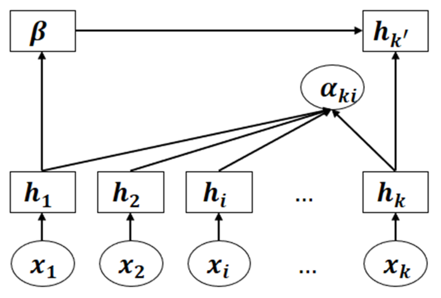
The model architecture of the attention mechanism in the GRU network is shown in Figure 2.
Where  x 1 , x 2 , x i , , x k  is the input sequence,  h 1 , h 2 , h i , , h k  is the state value of the GRU network,  α k i  is the attention distribution coefficient of the hidden layer state of the historical input information to the last state of the hidden layer,  β  is the weight of the whole hidden layer state, and  h k  is the hidden layer state of the last output node.
The core of the attention mechanism is to calculate the attention distribution coefficient  α k i , as shown in Formulas (8) and (9) [32]:
α k i = e x p e k i j = 1 l e x p e k j
e k i = V t a n h W h k + U h i
where  e k i  is the energy value of the hidden layer state at  i l  is the length of the input sequence, and  V ,   W ,  and  U  are the weight coefficient matrices that need to be trained in the network.
The semantic encoding and output feature vector that generate the attention distribution are shown in Formulas (10) and (11):
β = i = 1 l α k i h i
h k = H β , h k , x k

3. PQD Classification Based on CNN-GRU-P

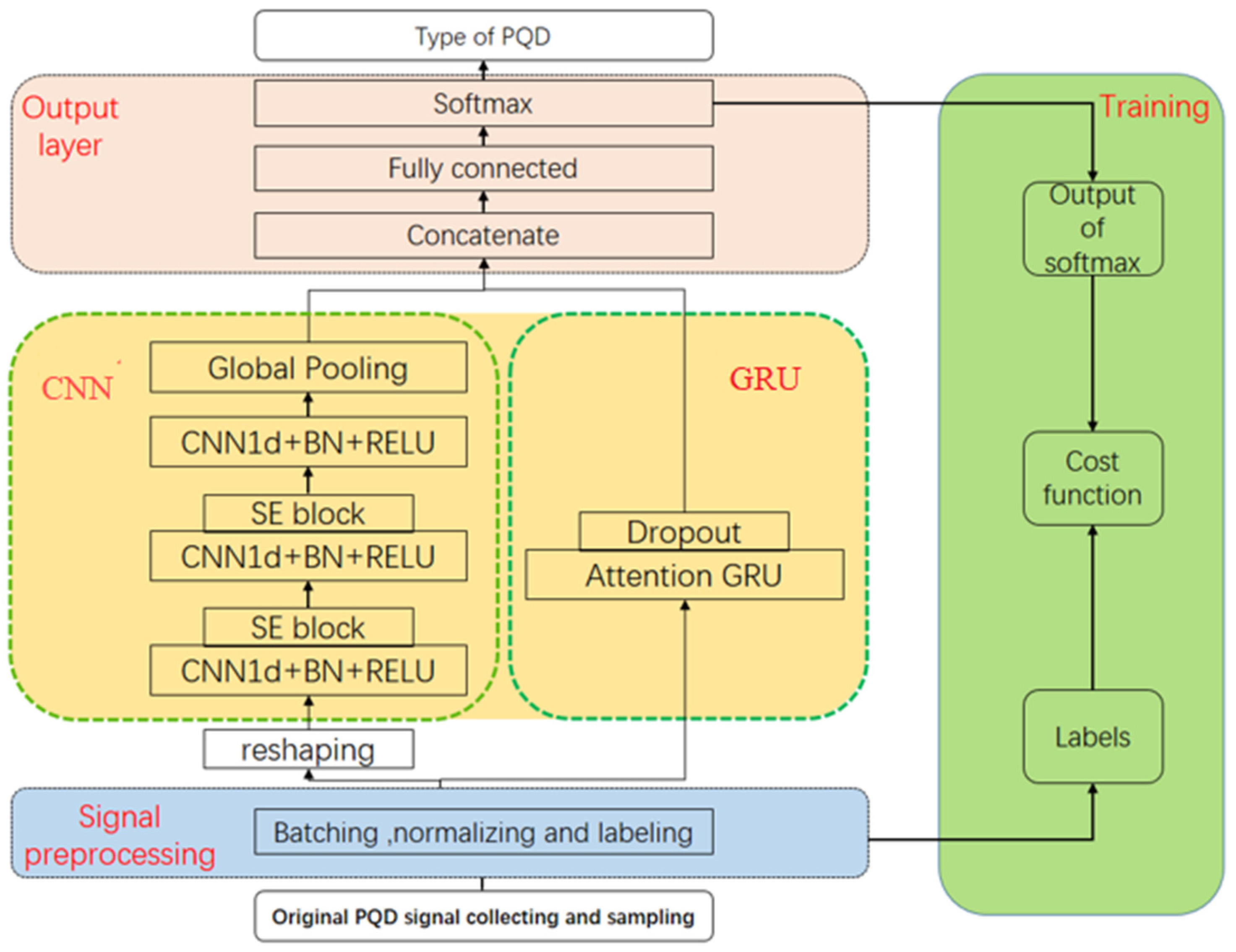
A “parallel” architecture network, referred to as CNN-GRU-P, which combines the advantages of the CNN and GRU neural networks, has been designed to extract both short-term and long-term features. The architecture of this network is illustrated in Figure 3. The proposed network consists of three layers: signal processing layer, CNN-GRU-P layer, and output layer.
To mitigate overfitting, we normalize each input PQD set by scaling it to a range of [0, 1]; we also assign corresponding labels to each PQD set and divide all PQDs into batches of size 128. The preprocessed PQDs are then fed into both the CNN and GRU networks for subsequent analysis.
Before inputting the PQD dataset into the CNN layer, the PQD dataset undergoes a reshaping process to convert its shape from (batch size, sequence length, 1) to (batch size, m, n), where n is the number of sampling periods in which the PQDs were obtained and m is the number of sampling points per cycle. This allows for the long PQD sequences to be divided into n shorter sequences of length m. This reshaping process improves the efficiency of network training.
The CNN comprises a stack of three convolutional blocks, two SE blocks, and a max average pooling layer. Each convolutional block includes a one-dimensional convolutional layer with a kernel size of 8, 5, and 3 and a number of filters of 128, 256, and 128, respectively. Each one-dimensional convolutional layer is followed by batch normalization with a momentum of 0.99 and epsilon of 0.001, and then the ReLU activation function. The first two convolutional blocks also include an SE block. The final convolutional block is followed by a global average pooling layer.
The GRU consists of a stack of GRU blocks and a dropout layer. The GRU block includes a GRU layer with 64 units and an attention embedding dimension of 128. The dropout rate is set to 80% to mitigate overfitting.
After the feature extraction, the short-term features from the CNN and long-term features from the GRU are concatenated using the Concat function and then input to a fully connected layer. Each concatenated PQD of features is used as an input to the fully connected layer, which applies the Softmax function to predict the PQD labels. The Adam optimizer [33] is used to calculate the loss between the model’s predictions and true labels, with a learning rate of 1 × 10⁻⁴.

4. Simulation and Analysis

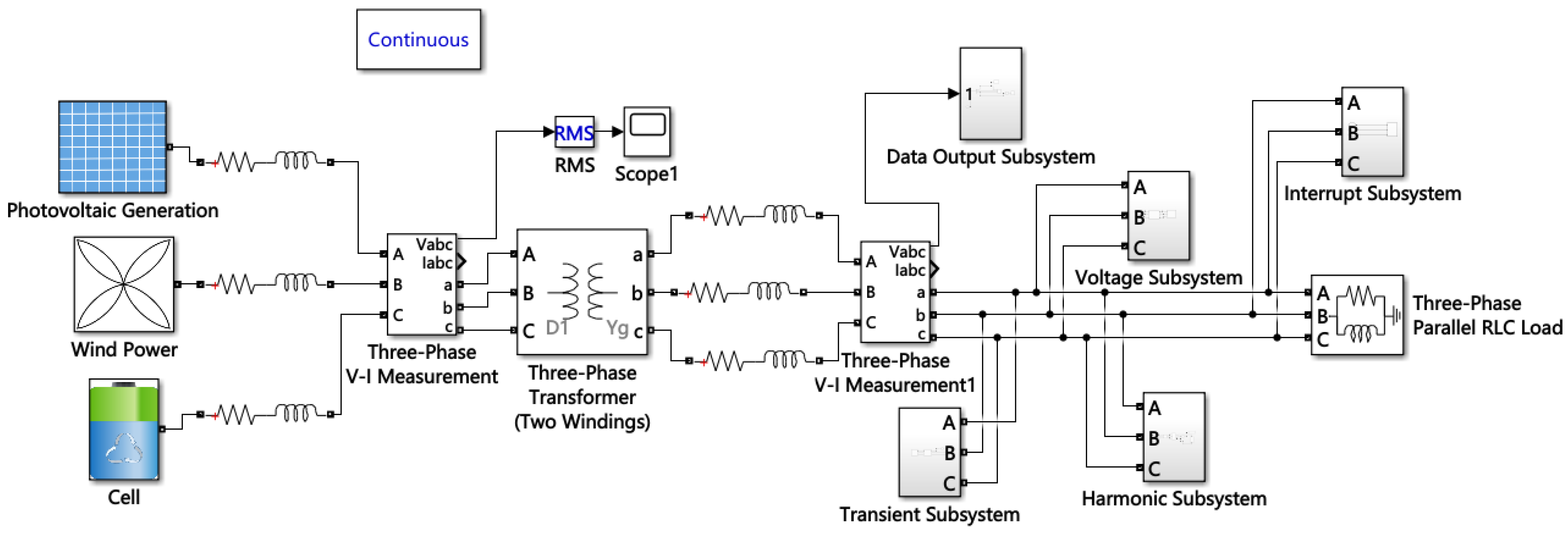
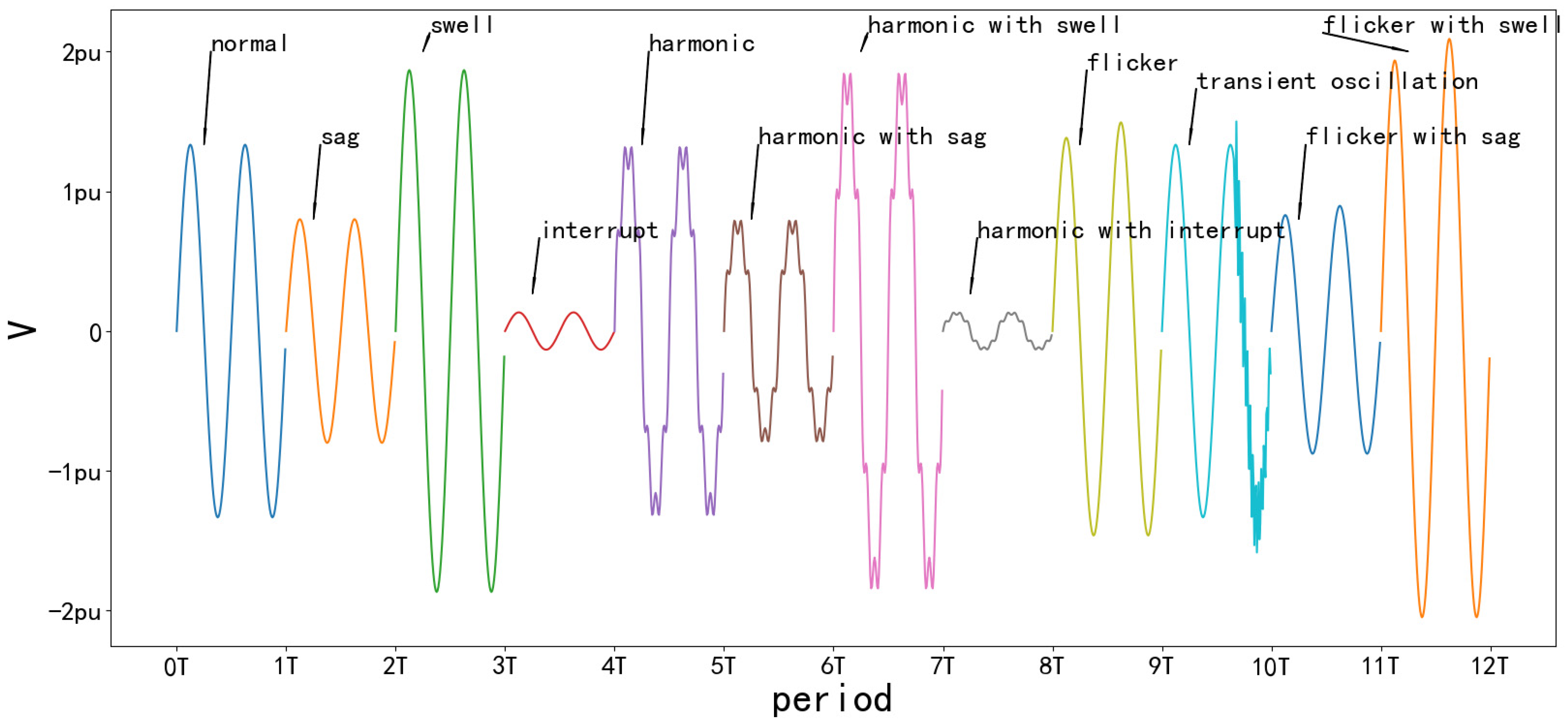
In this study, MATLAB-Simulink [34] was used to simulate the power grid. Figure 4 shows the microgrid model, which simulates the generation of PQDs in the power grid by setting the state of the components in the model [35]. Figure 5 illustrates twelve types of PQDs: six single PQDs, namely sag, swell, interrupt, transient, harmonic, and flicker, and six compound PQDs, namely harmonic with sag, harmonic with swell, harmonic with interrupt, flicker with sag, flicker with swell, and flicker with harmonic. Sag can be caused by a three-phase fault or switching of a large load. Swell can occur when large loads are suddenly removed from the system. Interrupt happens when there is a permanent three-phase fault. Transient can be created by switching a large capacitor bank. Harmonic is caused by three-phase nonlinear loads, and flicker can be created by connecting three-phase dynamic loads. Flicker is generated by changing the formula of the input power supply [36]. Compound PQDs can be simulated by combining single PQDs. The sampling frequency is set to 3200 Hz, and the data length of a single sample is 640 points. In total, 36,000 samples have been generated and divided into three sets, with 80% of the samples used for training, 10% for validating, and 10% for testing.
The proposed method was trained and evaluated using a computer with Intel(R) Core (TM) i7-10700 CPU @ 2.90 GHz, 16 GB DDR4 RAM, and NVIDIA Geforce GTX 1650 graphic card.
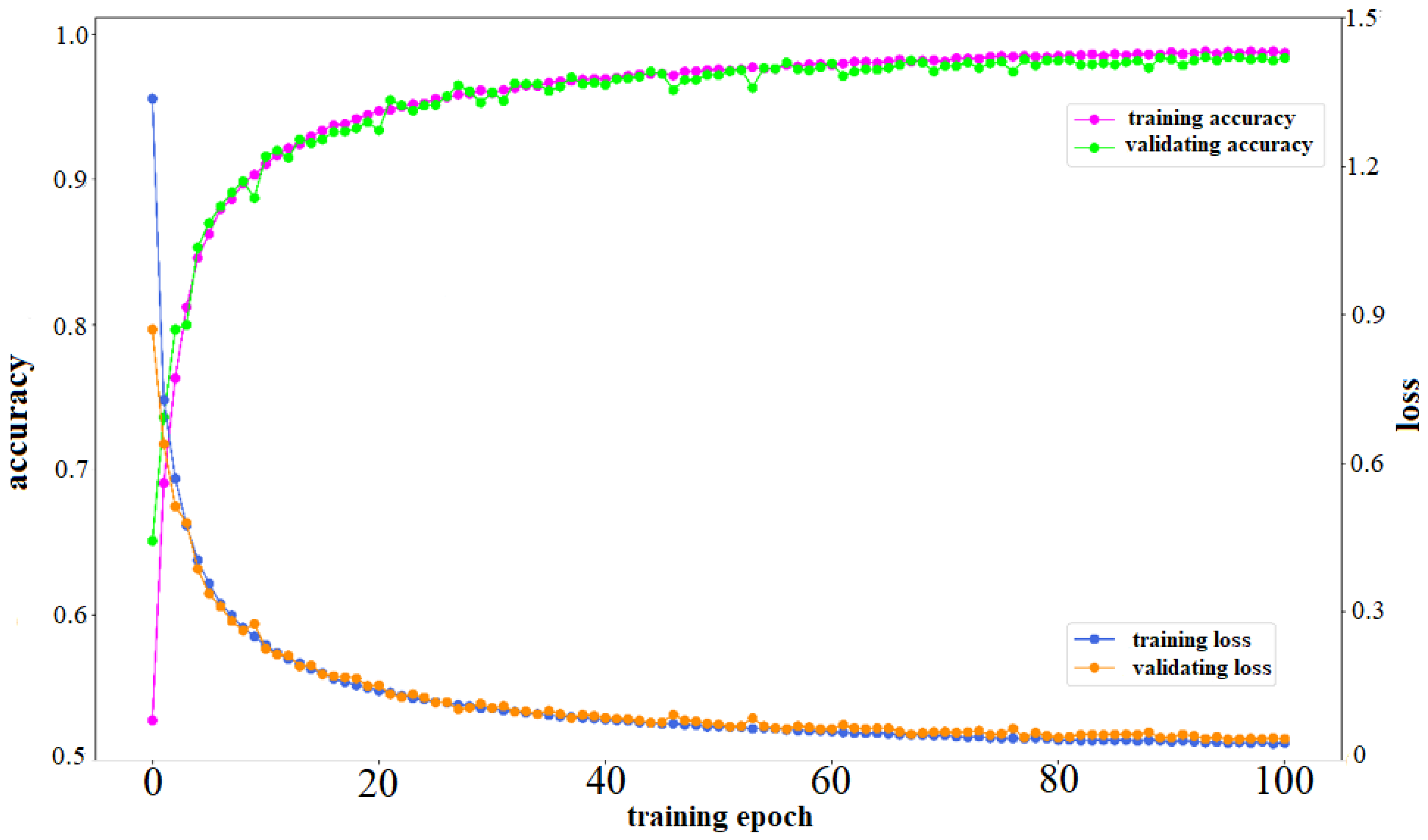
Figure 6 illustrates the accuracy and loss of CNN-GRU-P on both the training set and validation set. The training and validation accuracy of CNN-GRU-P increased, while the training and validation loss decreased. The training accuracy rate increased significantly from 52.7% to 98.7%, while the validation accuracy rate rose from 65.1% to 98.4%. In addition, the training loss decreased from 1.34 to 0.03, and the validation loss decreased from 0.87 to 0.04. These results suggest that the parameters of the network model are reasonable and that the training process is not overfitting the data.
The proposed network CNN-GRU-P along with CNN and GRU in series (called CNN-GRU-S) were first simulated and compared. Under zero-noise condition, the training time for CNN-GRU-P is 34 min and 42 s, while for CNN-GRU-S it is 24 min and 32 s. Despite the difference in training time, both networks have similar classification accuracy for a single PQD. However, there are differences in accuracy for compound PQDs between the two networks. For harmonic with sag, flicker with sag, and harmonic with swell, the accuracy in CNN-GRU-P is 99.9%, 99.0%, and 99.9%, respectively, while in CNN-GRU-S it is 89.5%, 87.6%, and 88.4%, respectively. While CNN-GRU-S has a shorter training time, CNN-GRU-P has demonstrated better performance in classifying compound PQDs, which is more representative of the real situation in a power grid. In order to further reflect the advantages of parallel connection, CNN-GRU-P is compared with CNN [17], GRU [19], and CNN-LSTM [20].
For the 12 PQDs mentioned above, three groups of data were sampled. One group of PQDs had noise, while the other two groups of PQDs had Gaussian noise added at 30 dB and 20 dB, respectively. The same dataset was used to train the CNN, GRU, CNN-LSTM, and CNN-GRU-P neural networks. The training times for these networks were 7 min and 46 s for CNN, 35 min and 29 s for GRU, 15 min and 4 s for CNN-LSTM, and 34 min and 42 s for CNN-GRU-P.
Table 1 displays the classification accuracy results of the CNN, GRU, CNN-LSTM, and CNN-GRU-P neural networks for three datasets.
Among the four neural networks, CNN has the lowest overall performance, but it demonstrates excellent recognition ability for oscillatory transients, achieving a 100% classification accuracy for this type of data. This is due to the strong feature extraction capability of the CNN. However, the CNN is limited in its ability to extract temporal features from PQDs, which ultimately restricts further improvements in classification accuracy.
The GRU network achieved an average accuracy of 89.2% on the 20 dB dataset, which is 4.7% higher than the average accuracy of CNN, which was 84.5%. These results demonstrate that the GRU has a strong anti-noise performance. Unlike CNN, GRU is capable of obtaining temporal features from PQDs, which contributes to its performance.
The CNN-LSTM network achieved an average accuracy of 97.0% on the 20 dB dataset. The classification accuracy of CNN-LSTM on the 20 dB noise dataset is 12.5% higher than that of CNN and 7.8% higher than that of LSTM. These results suggest that CNN-LSTM has excellent noise immunity. By combining CNN for feature extraction and LSTM for filtering and updating features, CNN-LSTM demonstrates a stronger feature extraction ability compared to CNN and LSTM.
The CNN-GRU-P network outperformed the other three neural networks on all three datasets, achieving an average classification accuracy that is higher than theirs. Moreover, the CNN-GRU-P network achieved a remarkable accuracy of 99.6% on the noise-free dataset. For the single PQDs, the CNN-GRU-P network demonstrated high accuracies, achieving 99.4%, 99.8%, 94.8, 100%, 98.5%, and 99.9% for sag, swell, interrupt, oscillatory transient, harmonic, and flicker, respectively. For compound PQDs, the CNN-GRU-P network achieved accuracies of 98.6%, 98.8%, 95.9%, 97.2%, 97.5%, and 95.9% for harmonic with sag, harmonic with swell, harmonic with interrupt, flicker with sag, flicker with swell, and flicker with harmonic, respectively. The results clearly demonstrate the effectiveness of the CNN-GRU-P network in detecting and classifying PQDs. Compared to the other three neural networks, the CNN-GRU-P network achieved a higher overall classification accuracy, and it also demonstrated better performance on compound disturbances. In particular, the CNN-GRU-P network achieved an average accuracy of 98.3% and 99.1% on the 20 dB and 30 dB noise datasets, respectively, indicating its strong anti-noise interference ability. These findings suggest that the CNN-GRU-P network is a promising approach for detecting and classifying PQDs in power systems.
The CNN-GRU-P network combines the strong feature extraction capability of the CNN with the ability of the GRU to extract time series features, making it a powerful approach for detecting and classifying PQDs. Unlike CNN-LSTM, which uses a “series” combination of a CNN and LSTM, CNN-GRU-P can simultaneously extract features from both the CNN and the GRU, enabling it to obtain complete time series features. Moreover, the SE block enhances the network’s ability to extract characteristic signals on different convolution channels, while the attention mechanism strengthens the GRU’s ability to extract timing signals of long timing signals such as PQDs. These features make CNN-GRU-P a highly effective approach for detecting and classifying PQDs in power systems.

5. Conclusions

(1)
This article proposes a novel parallel neural network (CNN-GRU-P) that combines a CNN with SE blocks and a GRU network with an attention mechanism for the classification of PQDs. The CNN-GRU-P method leverages the short-term feature extraction ability of a CNN and the long-term feature extraction ability of a GRU, while adding SE modules and attention mechanisms to enhance the network’s training efficiency. The end-to-end training processes of the network enable automatic feature extraction and selection, merging and replacing existing feature extraction, selection, and classification in the network. Experimental results demonstrate that the classification accuracy of the CNN-GRU-P network in single and composite disturbances outperforms other networks and exhibits good noise resistance. The application of this classification network to power quality classification can improve power quality and ensure the operational reliability of multi-energy systems. It should be noted that the proposed network structure is relatively complex, resulting in longer training times and requiring good training equipment. Nonetheless, the CNN-GRU-P method demonstrates promising results and has the potential to contribute significantly to the field of power quality classification.
(2)
A simulation model was established to analyze the factors leading to microgrid PQDs, such as three-phase faults, nonlinear loads, and large capacitor banks. The simulation results show that this method is suitable for accurately identifying single and composite power quality disturbances and provides a feasible solution for solving serious power quality problems in microgrids.

Author Contributions

Conceptualization, H.J.; methodology, H.J.; software, K.Z.; validation, K.Z.; formal analysis, J.C.; investigation, K.Z.; resources, K.Z.; data curation, K.Z.; writing—original draft preparation, J.C.; writing—review and editing, K.Z. and J.C.; visualization, J.C.; supervision, J.C.; project administration, H.J.; funding acquisition, H.J. All authors have read and agreed to the published version of the manuscript.

Funding

This research was funded by the Shenzhen Science and Technology Innovation Foundation under Grant JCYJ20190808165201648.

Data Availability Statement

The data generated by MATLAB-Simulink have been clearly stated in Section 4.

Conflicts of Interest

The authors declare no conflict of interest.

References

  1. Zhu, R.; Gong, X.; Hu, S.; Wang, Y. Power Quality Disturbances Classification via Fully-Convolutional Siamese Network and k-Nearest Neighbor. Energies 2019, 12, 4732. [Google Scholar] [CrossRef]
  2. Oubrahim, Z.; Amirat, Y.; Benbouzid, M.; Ouassaid, M. Power Quality Disturbances Characterization Using Signal Processing and Pattern Recognition Techniques: A Comprehensive Review. Energies 2023, 16, 2685. [Google Scholar] [CrossRef]
  3. Liao, J.; Zhou, N.; Wang, Q.; Li, C.; Yang, J. Definition and correlation analysis of DC distribution network power quality indicators. Proc. CSEE 2018, 38, 6847–6860+7119. [Google Scholar]
  4. Kumar, R.; Singh, B.; Shahani, D.T. Symmetrical Components-Based Modified Technique for Power-Quality Disturbances Detection and Classification. IEEE Trans. Ind. Appl. 2016, 16, 3443–3450. [Google Scholar] [CrossRef]
  5. Zhang, Y.; Zhang, Y.; Zhou, X. Classification of power quality disturbances using visual attention mechanism and feed-forward neural network. Measurement 2022, 188, 110390. [Google Scholar] [CrossRef]
  6. Wright, P.S. Short-time Fourier transforms and Wigner-Ville distributions applied to the calibration of power frequency harmonic analyzers. IEEE Trans. Instrum. Meas. 1999, 48, 475–478. [Google Scholar] [CrossRef]
  7. Grossmann, A.; Morlet, J. Decomposition of Hardy Functions into Square Integrable Wavelets of Constant Shape. Math. Anal. 1984, 15, 723–736. [Google Scholar] [CrossRef]
  8. Abdelsalam, A.A.; Eldesouky, A.A.; Sallam, A.A. Characterization of power quality disturbances using hybrid technique of linear Kalman filter and fuzzy-expert system. Electr. Power Syst. Res. 2012, 83, 41–50. [Google Scholar] [CrossRef]
  9. Stockwell, R.G.; Mansinha, L.; Lowe, R.P. Localization of the complex spectrum: The S transform. IEEE Trans. Signal Process. 1996, 44, 998–1001. [Google Scholar] [CrossRef]
  10. Huang, N.E.; Shen, Z.; Long, S.R.; Wu, M.C.; Shih, H.H.; Zheng, Q.; Yen, N.; Tung, C.C.; Liu, H.H. The empirical mode decomposition and the Hilbert spectrum for nonlinear and non-stationary time series analysis. Proc. R. Soc. Lond. Ser. A 1998, 454, 903–995. [Google Scholar] [CrossRef]
  11. Huang, N.; Peng, H.; Cai, G.; Xu, D. Power quality composite disturbance feature selection and Optimal Decision Tree construction. Proc. CSEE 2017, 37, 776–786. [Google Scholar]
  12. Cortes, C.; Vapnik, V. Support-vector networks. Mach. Learn. 1995, 20, 273–297. [Google Scholar] [CrossRef]
  13. Yi, L.; Li, K.; Li, L.; Chen, Z.; Meng, Q. Three-Layer Bayesian Network for Classification of Complex Power Quality Disturbances. IEEE Trans. Ind. Inform. 2018, 14, 3997–4006. [Google Scholar]
  14. Wang, H.; Wang, P.; Liu, T.; Zhang, B. Power quality disturbance classification based on growth-pruning optimized RBF neural network. Power Syst. Technol. 2018, 42, 2408–2415. [Google Scholar]
  15. Breiman, L. Random Forests. Machine Learning 2001, 45, 5–32. [Google Scholar] [CrossRef]
  16. Giri, A.K.; Arya, S.R.; Maurya, R.; Babu, B.C. Power Quality Improvement in Stand-alone SEIG based Distributed Generation System using Lorentzian Norm Adaptive Filter. IEEE Trans. Ind. Appl. 2018, 54, 5256–5266. [Google Scholar] [CrossRef]
  17. Garcia, C.I.; Grasso, F.; Luchetta, A.; Piccirilli, M.C.; Talluri, G. A Comparison of Power Quality Disturbance Detection and Classification Methods Using CNN, LSTM and CNN-LSTM. Appl. Sci. 2020, 10, 6755. [Google Scholar] [CrossRef]
  18. Fukushima, K. Neocognitron: A self-organizing neural network model for a mechanism of pattern recognition unaffected by shift in position. Biol. Cybern. 1980, 36, 193–202. [Google Scholar] [CrossRef]
  19. Qiu, W.; Tang, Q.; Liu, J.; Yao, W. An Automatic Identification Framework for Complex Power Quality Disturbances Based on Multi-fusion Convolutional Neural Network. IEEE Trans. Ind. Inform. 2020, 16, 3233–3241. [Google Scholar] [CrossRef]
  20. Deng, Y.; Wang, L.; Jia, H.; Tong, X.; Li, F. A Sequence-to-Sequence Deep Learning Architecture Based on Bidirectional GRU for Type Recognition and Time Location of Combined Power Quality Disturbance. IEEE Trans. Ind. Inform. 2019, 15, 4481–4493. [Google Scholar] [CrossRef]
  21. Cho, K.; Merrienboer, B.V.; Gulcehre, C.; Bahdanau, D.; Bougares, F.; Schwenk, H.; Bengio, Y. Learning Phrase Representations using RNN Encoder-Decoder for Statistical Machine Translation. arXiv 2014, arXiv:1406.1078. [Google Scholar]
  22. Junior, W.L.R.; Borges, F.A.S.; Rabelo, R.D.A.L.; Lima, B.V.A.D.; Alencar, J.E.A.D. Classification of Power Quality Disturbances Using Convolutional Network and Long Short-Term Memory Network. In Proceedings of the 2019 International Joint Conference on Neural Networks (IJCNN), Budapest, Hungary, 14–19 July 2019; pp. 1–6. [Google Scholar]
  23. Mohan, N.; Soman, K.P.; Vinayakumar, R. Deep power: Deep learning architectures for power quality disturbances classification. In Proceedings of the 2017 International Conference on Technological Advancements in Power and Energy (TAP Energy), Kollam, India, 21–23 December 2017; pp. 1–6. [Google Scholar]
  24. Hochreiter, S.; Schmidhuber, J. Long Short-Term Memory. Neural Comput. 1997, 9, 1735–1780. [Google Scholar] [CrossRef]
  25. Kumar, R.; Singh, B.; Shahani, D.T.; Chandra, A.; Al-Haddad, K. Recognition of Power-Quality Disturbances Using S-Transform-Based ANN Classifier and Rule-Based Decision Tree. IEEE Trans. Ind. Appl. 2015, 51, 1249–1258. [Google Scholar] [CrossRef]
  26. Wang, S.; Chen, H. A novel deep learning method for the classification of power quality disturbances using deep convolutional neural network. Appl. Energy 2019, 235, 1126–1140. [Google Scholar] [CrossRef]
  27. Karim, F.; Majumdar, S.; Darabi, H.; Chen, S. LSTM Fully Convolutional Networks for Time Series Classification. IEEE Access 2018, 6, 1662–1669. [Google Scholar] [CrossRef]
  28. Ioffe, S.; Szegedy, C. Batch Normalization: Accelerating Deep Network Training by Reducing Internal Covariate Shift. arXiv 2015, arXiv:1502.03167. [Google Scholar]
  29. Jie, H.; Li, S.; Gang, S.; Albanie, S. Squeeze-and-Excitation Networks. IEEE Trans. Pattern Anal. Mach. Intell. 2020, 42, 2011–2023. [Google Scholar]
  30. Chung, J.; Gulcehre, C.; Cho, K.H.; Bengio, Y. Empirical Evaluation of Gated Recurrent Neural Networks on Sequence Modeling. arXiv 2014, arXiv:1412.3555. [Google Scholar]
  31. Tolosana, R.; Vera-Rodriguez, R.; Fierrez, J.; Ortega-Garcia, J. Exploring Recurrent Neural Networks for On-Line Handwritten Signature Biometrics. IEEE Access 2018, 6, 5128–5138. [Google Scholar] [CrossRef]
  32. Luong, M.T.; Pham, H.; Manning, C.D. Effective Approaches to Attention-based Neural Machine Translation. arXiv 2015, arXiv:1508.04025. [Google Scholar]
  33. Kingma, D.; Ba, J. Adam: A Method for Stochastic Optimization. arXiv 2015, arXiv:1412.6980. [Google Scholar]
  34. Sun, Z. Introduction to Simulink Simulation and Code Generation Technology to Proficiency; Beihang University Press: Beijing, China, 2015. [Google Scholar]
  35. Dhote, P.V.; Deshmukh, B.T.; Kushare, B.E. Generation of power quality disturbances using MATLAB-Simulink. In Proceedings of the 2015 International Conference on Computation of Power, Energy, Information and Communication (ICCPEIC), Melmaruvathur, India, 22–23 April 2015; pp. 0301–0305. [Google Scholar]
  36. Zhang, Q.; Liu, H. Application of LS-SVM in Classification of Power Quality Disturbances. Proc. CSEE 2008, 28, 106–110. [Google Scholar]
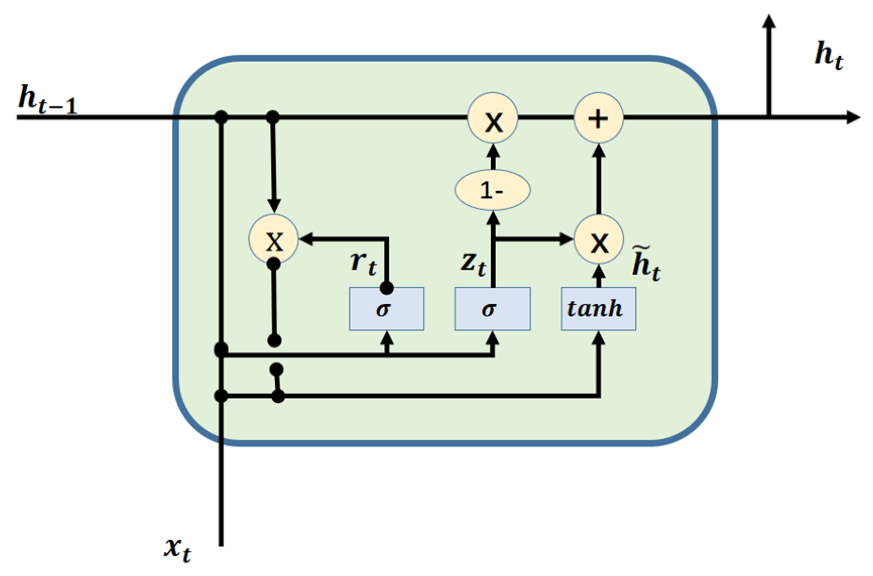
Figure 1. The architecture of GRU.
Energies 16 04029 g001
Figure 2. The attention mechanism in the GRU network.
Energies 16 04029 g002
Figure 3. The architecture of CNN-GRU-P.
Energies 16 04029 g003
Figure 4. Microgrid model for simulation.
Energies 16 04029 g004
Figure 5. Twelve typical PQDs.
Energies 16 04029 g005
Figure 6. The training process.
Energies 16 04029 g006
Table 1. The accuracy comparisons of CNN, GRU, CNN-LSTM, and CNN-GRU-P.
CNNGRUCNN-LSTMCNN-GRU-P’
Types of Disturbances20 dB30 dBNo
Noise
20 dB30 dBNo Noise20 dB30 dBNo Noise20 dB30 dBNo Noise
Sag75.393.799.282.797.999.798.999.599.599.499.8100.0
Swell90.299.899.993.094.3100.099.899.8100.099.899.999.9
Interrupt90.798.099.8100.099.798.795.799.5100.094.899.199.9
Oscillatory Transient100.0100.0100.099.099.7100.0100.0100.0100.0100.0100.0100.0
Harmonic84.383.188.079.784.095.794.591.394.098.598.699.5
Flicker86.997.899.988.394.3100.099.9100.0100.099.9100.0100.0
Harmonic with Sag86.293.998.388.391.799.797.399.499.498.699.799.8
Harmonic with Swell85.997.299.484.085.096.798.099.499.898.899.9100.0
Harmonic with Interrupt83.693.098.896.782.398.393.895.199.595.996.099.0
Flicker with Sag53.071.078.778.388.394.392.293.094.597.298.098.9
Flicker with Swell82.188.788.688.088.093.394.590.096.897.598.497.9
Flicker with Harmonic83.693.098.896.782.398.393.895.199.595.996.099.0
Average84.592.895.789.292.198.097.097.298.698.399.199.6
Disclaimer/Publisher’s Note: The statements, opinions and data contained in all publications are solely those of the individual author(s) and contributor(s) and not of MDPI and/or the editor(s). MDPI and/or the editor(s) disclaim responsibility for any injury to people or property resulting from any ideas, methods, instructions or products referred to in the content.