Maximum Power Tracking Control of Wind Turbines Based on a New Prescribed Performance Function

Abstract

The primary control goals of a wind turbine (WT) are structural load shedding, maximum wind energy capture in the underpowered situation, and consistent power production in the full power condition. A crucial component of the control problem for wind turbines with varying speeds is maximum power tracking control. Conventional maximum power tracking control tracks the ideal blade tip speed ratio to provide the most wind power at the specified wind speeds. However, because of the wind turbine’s great nonlinearity and the significant external disturbances it encounters, it is difficult to react quickly to variations in wind speed, and the tracking speed is sluggish, which lowers the amount of electricity produced annually. In light of this, this work develops a novel preset performance controller for a wind power system maximum power tracking control. With this technique, the convergence rate and tracking precision may be set. In particular, based on the concept of time-varying feedback, a time-varying function, known as the preset performance function, is first created to allow the convergence speed and accuracy to be predetermined; then this time-varying function is used to transform the actual specified time problem of the original system into a bounded time problem of the new system; finally, a direct robust controller design strategy with pre-defined performance is suggested based on the design concept of the backstepping technique. The plan may maximize the rotor power coefficient by altering the wind turbine speed, track the ideal blade tip speed ratio for a given tracking accuracy and speed, and get the most wind power to produce the most power with the strongest robustness. The simulation results show that the recommended control technique works.

1. Introduction

Wind energy is a green and renewable energy source, and the process of generating electricity from wind does not produce any carbon emissions. It is one of the power generation methods with the greatest potential [1]. Wind power generation will unavoidably play a significant role in the worldwide development of clean energy in order to fulfill the objectives of peak carbon and carbon neutrality, accelerate the proportion of renewable energy consumption, decrease the use of fossil fuels, and build a green and hospitable environment. The control of wind turbines has also received a great deal of attention in Europe and in some other countries around the world.

Generally speaking, there are two control loops to control a wind turbine, namely torque control loop and pitch control loop [2]. Figure 1 shows that, depending on the wind speed, the control of a wind turbine may be roughly split into three phases, i.e., the standby segment, the optimal Cp segment, and the rated power segment. The green line depicts the turbine’s actual operating curve, while the blue line shows that the turbine is running at its ideal blade tip speed ratio. Region 1 denotes that the turbine is in standby mode, since the wind speed is too low to generate electricity, with the rotational speed rising and the torque at 0. Region 2 is the optimal Cp section, where the blade tip speed ratio is ideal and the turbine has not yet reached its rated output. The turbine is controlled to maintain constant power by altering the pitch angle and generator torque in Region 3, which shows that the turbine has reached rated power and that the rotational speed is inversely proportional to the torque. Area 1_1/2 indicates the start-up state and area 2_1/2 the transition state where the rated power is about to be reached, these two areas account for very little. The region 2 is under power operation. To utilise wind energy as much as possible in this operating region is the control aim. At this stage, the blade pitch angle is locked at the optimal value in order to optimize power production, and the torque control circuit is used to adjust the rotor speed to run relatively near to the ideal speed. Numerous control techniques, including tip speed ratio (TSR) control [3], optimal torque control [4], power signal feedback control [5], and extremum seeking control [6], etc., have been researched and used in this sector. However, their characteristics include a slow tracking speed and that tracking accuracy cannot be set in advance.

In control engineering, a common control goal is trajectory tracking [7]. The convergence rate and the final tracking error range, two crucial metrics for assessing the controller, must frequently be taken into account when developing a controller. The tracking error needs to converge to a specified precision within a given period for several application scenarios that have higher criteria for safety and reliability, such as target interception, spacecraft docking, and auto parts assembly [1,8]. The latest results of prescribed time control [9,10,11,12,13] solve the problem of system stability in a limited time. The designer can predefine the convergence time, which is a parameter that is independent of the initial situation. Using this method, the control gain is engineered to grow infinitesimally as time moves closer to the terminal time T, resulting in the desired temporal stability [14]. It is challenging to build controllers for systems with the majority of uncertainties and external disturbances in order to achieve zero error tracking. In fact, in practical engineering applications, the tracking error is allowed to have an appropriate accuracy range rather than zero error. Due to this, a few scholars have proposed a useful theory of finite-time control in which the tracking error converges in limited time to a local neighborhood (rather than zero) of the origin [15,16,17,18,19,20,21,22,23]. The tracking error after the stabilization time is uncertain since the size of this neighborhood is unknown, and its value actually depends on some unknowable factors. In the field of engineering, this is quite undesirable.

In order to obtain the maximum power output of a wind turbine at low wind speeds, we attempt to create a new prescribed performance controller (PPC) based on the discussion above. No matter what the initial conditions are, users can fully specify the convergence speed and tracking accuracy in advance. In order to allow the designer to set the convergence rate and accuracy in advance, we first create a time-varying function, known as a prescribed performance function (PPF), with embedded stability time and tracking accuracy. Then, we use this time function to transform the actual specified time problem of the original system into the bounded time problem of the new system. Finally, derived from the design idea of the backstepping method [24], we propose a direct robust controller (DRC) design scheme.

The contributions of this paper include: (1) The convergence rate and tracking precision can both be predetermined by the designer utilizing the new error transformation based on PPF; (2) Not only the tracking error variable, but also all other intermediate error variables will reach the predetermined stable region within a given time; (3) In spite of external disturbance, the WT can respond to the change of wind speed quickly and achieve maximum power control.

2. Preliminaries and Problem Formulation

2.1. Problem Formulation

Take into account the following uncertain nonlinear strict-feedback systems:

$$\{\begin{array}{l}{\dot{x}}_i=f_i\left({\overline{x}}_i\right)+g_i\left({\overline{x}}_i\right)x_{i+1}+d_i,i=1,\dots ,n-1\\ {\dot{x}}_n=f_n\left({\overline{x}}_n\right)+g_n\left({\overline{x}}_n\right)u+d_n\\ y=x_1\end{array}$$

(1)

where ${\overline{x}}_i={\left[x_1,x_2,\cdots ,x_i\right]}^T\in {ℝ}^i$ is the system state; $u\in ℝ$ and $y$ are the system input and the system output, respectively; $f_i\left({\overline{x}}_i\right)$ and $g_i\left({\overline{x}}_i\right)$ represent the uncertain nonlinear continuous function and unknown gain function, respectively; $d_i(.)$ denotes the unknown time-varying disturbances.

Designing a correct $u$ to achieve the following objectives is the main task of this paper:

(a)

In closed-loop systems, the intermediate signals are constrained;

(b)

The preset performance tracking (PPT) is achieved, i.e., there are matching parameter values for every $\epsilon >0$ and $T>0$ ensuring $\left|w_1\left(t\right)\right|=\left|y\left(t\right)-y_d\left(t\right)\right|<\epsilon$ when $t\ge T$, where $y_d\left(t\right)$ is the target reference signal.

Certain assumptions are made in order to accomplish the aforementioned control aims.

Assumption 1.

The gain functions $g_i\left({\overline{x}}_i\right)$ are positive and there are unidentified constants $0<{\underset{\_}{g}}_i<{\overline{g}}_i$ that case $0<{\underset{\_}{g}}_i\le g_i\left({\overline{x}}_i\right)\le {\overline{g}}_i$.

Assumption 2.

For lumped uncertainties there exist unknown constants $a_i$ and known functions ${\phi }_i\left({\overline{x}}_i\right)$ such that $f_i\left({\overline{x}}_i\right)\le a_i{\phi }_i\left({\overline{x}}_i\right)$.

Assumption 3.

The unknown time-varying disturbances $d_i(.)$ are bounded, and there exist unknown positive constant $D_i$ satisfy $\left|d_i(.)\right|\le D_i$.

Assumption 4.

The desired trajectory $y_d$ and its $i\left(i=1,\dots ,n\right)$-order derivatives are known, piecewise continuous and bounded.

2.2. Some Lemmas and Definitions

Lemma 1.

For any $\left|r\right|<1$, the following inequality holds:

$$\ln \left(\frac{1}{1-r^2}\right)\le \frac{r^2}{1-r^2}$$

Lemma 2

([11]). For constants $l>0$ and time-varying functions $v\left(t\right)>0$, there are:

$${\displaystyle {\int }_0^t{\exp }^{-l{\displaystyle {\int }_{\tau }^{t}v\left(s\right)ds}}v\left(\tau \right)d\tau \le \frac{1}{l}}$$

Definition 1

([25]). Semi-global Practical Prescribed Time (PPT) Stability: The practical prescribed time stability of nonlinear system, $\dot{x}=f\left(x\right)$ with $x$ being system state, is said to be reached if for any initial condition $x\left(0\right)=x_0$, there exist constant $\epsilon >0$ and finite time $T<\infty$ (in which $T$ is independent of systems initial conditions and other design parameter vector), such that $\left|x\right|<\epsilon$ for all $t>T$.

It can be seen from Definition 1 that the accuracy $\epsilon$ in the semi-global practical prescribed time (PPT) stability is not a specific value. In other words, there is no explicit need for the size of this domain; just that the system’s state converge to a finite error domain within a certain amount of time. The following practical predefined time and precision stability is defined as the tracking error being restricted to a predetermined compact set around zero within a stipulated period $T$.

Definition 2

([26]). If a time-varying function $\rho \left(t\right)$ holds the following generalized properties, then this function is called a new prescribed performance function (NPPF):

• $\rho \left(t\right)$ is a continuous and non–increasing $C^n$ function from an initial $\rho \left(0\right)={\rho }_0$ to a terminal value $\rho \left(T\right)=\epsilon$, where ${\rho }_0$, $\epsilon$, $T$ are given as constants greater than 0.
• $\dot{\rho }\left(T\right)=0$; When $t>T$, $\rho \left(t\right)=\epsilon$ and thus $\dot{\rho }\left(t\right)=0$.

Immediate examples of such $\rho \left(t\right)$ include the subsequent formulae with $t\ge 0$:

$$\rho =\{\begin{array}{l}{\left(\frac{T-t}{T}\right)}^m\left({\rho }_0-\epsilon \right)+\epsilon ,0\le t<T\\ \epsilon ,t\ge T\end{array},$$

$$\rho =\{\begin{array}{l}{\left(\frac{T-t}{T}\right)}^m{e}^{-t}\left({\rho }_0-\epsilon \right)+\epsilon ,0\le t<T\\ \epsilon ,t\ge T\end{array},$$

$$\rho =\{\begin{array}{l}{\sin }^m\left(\frac{\pi }{2}\frac{T-t}{T}\right)\left({\rho }_0-\epsilon \right)+\epsilon ,0\le t<T\\ \epsilon ,t\ge T\end{array}.$$

where the constant $m$ meets the $m\ge 2$ requirement. It should be noted that there are many functions that satisfy Definition 2, which are not limited to the above examples.

We build the following lemma to continue the control design because it will be vital to our later technological development.

2.3. Definition of a New Variable

Lemma 3.

We firstly define a new variable $h=r\ln \left(1-r^2\right)$, where $r=e/\rho$, $e=y-y_d$. If we can design an appropriate controller $u(.)$ so that $h$ bounded with the condition of the initial state satisfy $\left|e\left(0\right)\right|<{\rho }_0$, then we can get $-\rho <e<\rho$.

Proof of Lemma 3.

Contradiction is the method that we use to provide our proofs. Given that $\left|w\left(0\right)\right|<{\rho }_0$, $-\rho <e\left(0\right)<\rho$ obviously holds, which further implies that $-1<r\left(0\right)<1$. Suppose that $w\left(t\right)\le -\rho$ or $e\left(t\right)\ge \rho$ for $t=t_1$, thus we have $r\left(t_1\right)\le -1$ or $r\left(t_1\right)\ge -1$. Then, from the intermediate value theorem of continuous functions, there exists a time instant $0<t_2<t_1$ such that $r\left(t_2\right)=-1$ or $r\left(t_2\right)=1$. We obtain that $1-r^2\left(t_2\right)=0$, further resulting $h\left(t_2\right)=\infty$, which leads to a contradiction for the boundedness of $h$. Therefore, it is concluded that $-1<r\left(t\right)<1$ and $-\rho \left(t\right)<e\left(t\right)<\rho \left(t\right)$ for every $t\in [0,\infty )$. The proof ends here. □

3. Results

3.1. Modelling of Wind Turbines

A wind turbine is made up of four basic parts, including aerodynamics, mechanics, a generator, and a pitch actuator, as depicted in Figure 2. The two discs on the left and right in Figure 3 are the determinant of inertias, $J_r$ and $J_g$. In other words, $J_r$ and $J_g$ represent the rotor’s and the generator’s respective rotational inertia. The rotation of the rotor shaft at high torques is described as a mass-spring system with damping $D_s$ and a spring constant $K_s$. In addition, $T_r$ and $T_g$ stand for the torque on each side of the rotor and generator, respectively. The transmitted torques $T_{rs}$ and $T_{gs}$ are interconnected via the gear ratio $N_g$.

The aerodynamic model of a wind turbine is

$$\{\begin{array}{l}{P}_a=\frac{1}{2}\rho \pi R^2{v}^3{C}_p\left(\lambda ,\beta \right)\\ \lambda =\frac{R\omega }{v}\end{array}$$

(2)

where $\rho$ represents air density; $R$ represents rotor radius; and $v$ represents wind speed; the rotor power coefficient, denoted by the symbol $C_p\left(\lambda ,\beta \right)$, is as follows [27]:

$$C_p\left(\lambda ,\beta \right)=c_1\left(\frac{c_2}{{\lambda }_0}-c_3\beta -c_4\right)\exp \left(\frac{-c_5}{{\lambda }_0}\right)+c_6\lambda$$

(3)

$$\frac{1}{{\lambda }_0}=\frac{1}{\lambda +0.08\beta }-\frac{0.035}{{\beta }^3+1}$$

(4)

$${\omega }_d=\frac{{\lambda }_{opt}R}{v}$$

(5)

where ${\omega }_d$ is the optimal generator speed.

The single mass block model of the wind turbine drive train is as follows

$$J\dot{\omega }=T_a-r_g{T}_g-B\omega$$

(6)

$$T_a=K_a{\omega }^2$$

(7)

where $J$ is the total moment of inertia of the wind turbine; $K_a=1/2\rho \pi R^5{C}_p/{\lambda }^3$ is wind turbine’s operational state coefficient; $T_g$ is generator torque; $B$ is the total damping coefficient of the transmission system; $r_g$ is the gear ratio.

You may rewrite System (6) as

$$\dot{x}=f\left(x\right)+gu+d(.)$$

(8)

where $x=\omega$, $f\left(x\right)=-B/Jx$, $g=-r_g/Jg$, $d(.)=D(.)$, $u=T_g$.

3.2. Error Transformation

Based on Assumption 4 in Section 2.1, the tracking error is defined as:

$$w_1=y-y_d$$

(9)

Obviously, the control objective (b) holds if the controller can be designed so that the tracking error satisfies the following inequality:

$$-\rho <w_1<\rho$$

(10)

Then, we have $\left|w_1\right|<\epsilon$ for $t\ge T$.

Define the intermediate error variable as:

$$w_i=x_i-{\overline{\partial }}_{i-1},i=2,\dots ,n$$

(11)

where ${\overline{\partial }}_{i-1}$ stand for output signal of virtual controller ${\partial }_{i-1}$ to be designed through the first-order filter with variable time constant as follows:

$$\rho l_{i-1}{\dot{\overline{\partial }}}_{i-1}+{\overline{\partial }}_{i-1}={\partial }_{i-1},{\partial }_{i-1}\left(0\right)={\overline{\partial }}_{i-1}\left(0\right)$$

(12)

Filtering errors are defined as follows:

$${\varphi }_{i-1}={\overline{\partial }}_{i-1}-{\partial }_{i-1}$$

(13)

To guarantee that the error variables $w_i$ are constrained to the specified precision $\epsilon$ at the same rate, and that the system’s state $x_i$ does not go beyond a predetermined bound, we define the transformation error variable:

$$h_i=r_i\ln \left(1-r_i{}^2\right)$$

(14)

where $r_i=v{w}_i$, $v=1/\rho$. Take the derivative of $h_i$, the following transformation is performed on system (1):

$$\{\begin{array}{l}{\dot{h}}_1={\lambda }_1+{\pi }_1\left(f_1+g_1{w}_2+g_1{\varphi }_1+d_1-{\dot{x}}_d+g_1{\partial }_1\right)\\ {\dot{h}}_i={\lambda }_i+{\pi }_i\left(f_i+g_i{w}_{i+1}+g_i{\varphi }_i+d_i-{\dot{\overline{\partial }}}_{i-1}+g_n{\partial }_i\right),i=2,\dots ,n-1\\ {\dot{h}}_n={\lambda }_n+{\pi }_n\left(f_n+d_n-{\dot{\overline{\partial }}}_{n-1}+g_{n}u\right)\end{array}$$

(15)

where

$$\begin{array}{l}{\lambda }_i={\overline{\lambda }}_{i}v,{\overline{\lambda }}_i=-\left(\ln \left(1-r_i{}^2\right)+\frac{-2r_i{}^2}{1-r_i{}^2}\right)r_i\dot{\rho }\\ {\pi }_i=v{\overline{\pi }}_i,{\overline{\pi }}_i=\left(\ln \left(1-r_i{}^2\right)+\frac{-2r_i{}^2}{1-r_i{}^2}\right)\end{array}$$

(16)

According to Lemma 3 in Section 2.3, if the virtual controller $\partial =\left[{\partial }_1\cdots {\partial }_{n-1}\right]$ and controller $u(.)$ are designed to make the conversion error variable $h=\left[h_1\cdots h_n\right]$ bounded, then we will get $-\rho <w_i<\rho ,i=1,\dots ,n$. The PPT control issue of (1) is simplified to building a controller such that the state of the system shown in (15) is limited, hence simplifying the previously complex control problem.

3.3. Direct Robust Control (DRC) Scheme

The backstepping method divides a complex nonlinear system into subsystems no larger in size than the system itself, designs partial Lyapunov functions for each subsystem, “backstepping” all the way to the whole system, and then integrates them to finish designing the entire control law.

Step 1: From (15), it follows that

$${\dot{h}}_1={\lambda }_1+{\pi }_1\left(f_1+g_1{w}_2+g_1{\varphi }_1+d_1-{\dot{x}}_d+g_1{\partial }_1\right)$$

(17)

Then, the time derivative of $\frac{1}{2}{h}_1{}^2$ along (17) is

$$h_1{\dot{h}}_1=h_1{\lambda }_1+h_1{\pi }_1\left(f_1+g_1{w}_2+g_1{\varphi }_1+d_1-{\dot{x}}_d+g_1{\partial }_1\right)$$

(18)

It is simple to obtain that with the aid of Assumptions 1–3 in Section 2.1 and Young’s inequality [28]:

$$\begin{array}{l}{h}_1{\lambda }_1\le v{\underset{\_}{g}}_1{h}_1{}^2{\overline{\lambda }}^2{}_1+v\frac{1}{4{\underset{\_}{g}}_1}\\ h_1{\pi }_1{f}_1\le \left|h_1{\pi }_1\right|a_1{\phi }_1\le v{\underset{\_}{g}}_1{\phi }_1{}^2{h}_1{}^2{\overline{\pi }}_1{}^2+v\frac{a_1{}^2}{4{\underset{\_}{g}}_1}\\ h_1{\pi }_1{d}_1\le v{\underset{\_}{g}}_1{h}_1{}^2{\overline{\pi }}_1{}^2+v\frac{d_1{}^2}{4{\underset{\_}{g}}_1}\\ -h_1{\pi }_1{\dot{x}}_d\le v{\underset{\_}{g}}_1{h}_1{}^2{\overline{\pi }}_1{}^2{\dot{x}}_d{}^2+\frac{1}{4{\underset{\_}{g}}_1}\\ h_1{\pi }_1{g}_1{w}_2\le v\frac{g_1}{2}{h}_1{}^2{\overline{\pi }}_1{}^2{w}_2{}^2+v\frac{{\overline{g}}_1}{2}\le \rho \frac{g_1}{2}{h}_1{}^2{\overline{\pi }}_1{}^2+v\frac{{\overline{g}}_1}{2}\\ h_1{\pi }_1{g}_1{\varphi }_1\le v\frac{g_1}{2}{h}_1{}^2{\overline{\pi }}_1{}^2+v\frac{{\overline{g}}_1}{2}{\varphi }_1{}^2\end{array}$$

(19)

Adding the aforementioned disparities’ two sides gives us

$$h_1{\dot{h}}_1\le h_1{\pi }_1{g}_1{\partial }_1+v{\underset{\_}{g}}_1{h}_1{}^2{\overline{\pi }}_1{}^2\left(\frac{{\overline{\lambda }}_1{}^2}{{\overline{\pi }}_1{}^2}+{\phi }_1{}^2+{\dot{x}}_d{}^2+{\rho }^2+\frac{3}{2}\right)+v\frac{{\overline{g}}_1}{2}{\varphi }_1{}^2+v{\Delta }_1$$

(20)

where ${\Delta }_1=\frac{2+a_1{}^2+D_1{}^2}{4{\underset{\_}{g}}_1}+\frac{{\overline{g}}_1}{2}$. Hence the virtual control is constructed as

$${\partial }_1=-h_1\frac{{\overline{\lambda }}_1{}^2}{{\overline{\pi }}_1}-h_1{\overline{\pi }}_1{\phi }_1{}^2-h_1{\overline{\pi }}_1{\dot{x}}_d{}^2-\frac{1}{2}{h}_1{\overline{\pi }}_1{\rho }^2-\frac{3}{2}{h}_1{\overline{\pi }}_1-k_1{r}_1$$

(21)

where $k_1>0$. Using Lemma 1 in Section 2.2, we can get:

$$\begin{array}{l}-k_1{r}_1{h}_1{\pi }_1{g}_1=-k_{1}v{g}_1{h}_1\left(\ln \left(1-r_1{}^2\right)+\frac{-2r_1{}^2}{1-r_1{}^2}\right)r_1\\ =-k_{1}v{g}_1{r}_1{}^{2}ln(1-r_1{}^2)(ln(1-r_1{}^2)+\frac{-2r_1{}^2}{1-r_1{}^2})\\ =-k_{1}v{g}_1\left\{h_1{}^2+r_1{}^{2}ln(1-r_1{}^2)\frac{-2r_1{}^2}{1-r_1{}^2}\right\}\\ \le -3k_{1}v{\underset{\_}{g}}_1{h}_1{}^2\end{array}$$

(22)

Combining (16) and (21), we get

$$h_1{\pi }_1{g}_1{\partial }_1\le -v{\underset{\_}{g}}_1{h}_1{}^2{\overline{\pi }}_1{}^2\left(\frac{{\overline{\lambda }}_1{}^2}{{\overline{\pi }}_1{}^2}+{\phi }_1{}^2+{\dot{x}}_d{}^2+{\rho }^2+\frac{3}{2}\right)-3k_{1}v{\underset{\_}{g}}_1{h}_1{}^2$$

(23)

A candidate for a Lyapunov function is now defined as

$$V_1=\frac{1}{2}{h}_1{}^2+\frac{1}{2}{\varphi }_1{}^2$$

(24)

Differentiating (24) and combining (20)–(23), we have

$${\dot{V}}_1\le -3k_{1}v{\underset{\_}{g}}_1{h}_1{}^2+{\varphi }_1\dot{\varphi }+v\frac{{\overline{g}}_1}{2}{\varphi }_1{}^2+v{\Delta }_1$$

(25)

where ${\varphi }_1$ is the filtering error, and its derivative is:

$${\dot{\varphi }}_1=\frac{-{\varphi }_1}{l_1}v-{\dot{\partial }}_1=\frac{-{\varphi }_1}{l_1}v+{\kappa }_1\left(r_1,\rho ,\dot{\rho },x_d,{\dot{x}}_d,{\varphi }_1,{\phi }_1\right)$$

(26)

Each variables of the function ${\kappa }_1$ are in the compact sets, at the same time, ${\kappa }_1$ is a smooth function, it follows that the largest $\left|{\kappa }_1\right|$ is ${\overline{\kappa }}_1$, i.e., $\left|{\kappa }_1\right|<{\overline{\kappa }}_1$ with ${\overline{\kappa }}_1$ being an unknown constant. Thus, we have:

$${\varphi }_1{\dot{\varphi }}_1=\frac{-{\varphi }_1{}^2}{l_1}v-{\varphi }_1{\dot{\partial }}_1\le v\left\{-\left(\frac{1}{l_1}-\frac{{\rho }_0}{2}\right){\varphi }_1{}^2+\frac{{\overline{\kappa }}_1{}^2}{2}{\rho }_0\right\}$$

(27)

Substituting (27) into (25), we have

$$\begin{array}{l}{\dot{V}}_1\le -3k_{1}v{\underset{\_}{g}}_1{h}_1{}^2-v\left(\frac{1}{l_1}-\frac{{\rho }_0}{2}-\frac{{\overline{g}}_1}{2}\right){\varphi }_1{}^2+v{\Delta }_1\\ \le -{\overline{k}}_{1}v{V}_1+v{\Delta }_1,{\overline{k}}_1=\min \left\{6k_1{\underset{\_}{g}}_1,\frac{2}{l_1}-{\rho }_0-{\overline{g}}_1\right\}\end{array}$$

(28)

Step $i\left(i=2,\mathrm{\dots },n-1\right)$. Similar to step 1, combined with the system (15), $\frac{1}{2}{h}_i{}^2$ derivative of time is:

$$h_i{\dot{h}}_i=h_i{\lambda }_i+h_i{\pi }_i\left(f_i+g_i{w}_{i+1}+g_i{\varphi }_i+d_i-{\dot{\overline{\partial }}}_{i-1}+g_i{\partial }_i\right)$$

(29)

The virtual controller is designed as

$${\partial }_i=-h_i\frac{{\overline{\lambda }}^2{}_i}{{\overline{\pi }}_i}-h_i{\overline{\pi }}_i{\phi }_i{}^2-h_i{\overline{\pi }}_i{\dot{\overline{\partial }}}^2{}_{i-1}-\frac{1}{2}{h}_i{\overline{\pi }}_i{\rho }^2-\frac{3}{2}{h}_i{\overline{\pi }}_i-k_i{r}_i$$

(30)

Define a positive definite Lyapunov function

$$V_i=\frac{1}{2}{h}_i{}^2+\frac{1}{2}{\varphi }_i{}^2$$

(31)

Differentiating (31) and combining (29), we have

$${\dot{V}}_i=h_i{\lambda }_i+h_i{\pi }_i\left(f_i+g_i{w}_{i+1}+g_i{\varphi }_i+d_i-{\dot{\overline{\partial }}}_{i-1}+g_i{\partial }_i\right)+{\varphi }_1{\dot{\varphi }}_1$$

(32)

With the help of Young’s inequality and also considering the approach described in (19), we have

$$\begin{array}{l}{h}_i{\lambda }_i+h_i{\pi }_i(f_i+g_i{w}_{i+1}+g_i{\varphi }_i+d_i-{\dot{\overline{\partial }}}_{i-1})\le \frac{1}{\rho }{\underset{\_}{g}}_i{h}_i{}^2{\overline{\pi }}_i{}^2(\frac{{\overline{\lambda }}^2{}_i}{{\overline{\pi }}_i{}^2}+{\phi }_i{}^2+{\dot{\overline{\partial }}}_{i-1}{}^2+{\rho }^2+\frac{3}{2})+v{\Delta }_i\\ h_i{\pi }_i{g}_i{\partial }_i\le -v{\underset{\_}{g}}_i{h}_i{}^2{\overline{\pi }}_i{}^2\left(\frac{{\overline{\lambda }}_i{}^2}{{\overline{\pi }}_i{}^2}+{\phi }_i{}^2+{\dot{\overline{\partial }}}_{i-1}{}^2+{\rho }^2+\frac{3}{2}\right)-3k_i\rho {\underset{\_}{g}}_i{h}_i{}^2\end{array}$$

(33)

where ${\Delta }_i=\frac{2+a_i{}^2+D_i{}^2}{4{\underset{\_}{g}}_i}+\frac{{\overline{g}}_i}{2}$.

Using a similar approach as in Step 1, we have

$${\dot{\varphi }}_i=\frac{-{\varphi }_i}{l_i}v+{\kappa }_i\left(r_1,\dots ,r_i,\rho ,\dot{\rho },x_d,{\dot{x}}_d,{\varphi }_i,{\phi }_1,\dots ,{\phi }_i\right)$$

(34)

and the largest $\left|{\kappa }_1\right|$ is ${\overline{\kappa }}_1$, i.e., $\left|{\kappa }_i\right|<{\overline{\kappa }}_i$ with ${\overline{\kappa }}_i$ being an unknown constant. Therefore, it is possible to obtain that:

$${\varphi }_i{\dot{\varphi }}_i=\frac{-{\varphi }_i{}^2}{l_i}v-{\varphi }_i{\dot{\partial }}_i\le -v\left(\frac{1}{l_i}-\frac{{\rho }_0}{2}\right){\varphi }_i{}^2+\frac{{\overline{\kappa }}_i{}^2}{2}{\rho }_{0}v$$

(35)

Substituting (33) and (35) into (32), we get:

$${\dot{V}}_i\le -3k_{i}v{\underset{\_}{g}}_i{h}_i{}^2-v\left(\frac{1}{l_i}-\frac{{\rho }_0}{2}-\frac{{\overline{g}}_i}{2}\right){\varphi }_i{}^2+v{\Delta }_i\le -{\overline{k}}_{i}v{V}_1+v{\Delta }_i$$

(36)

where ${\overline{k}}_i=\min \left\{6k_i{\underset{\_}{g}}_i,\frac{2}{l_i}-{\rho }_0-{\overline{g}}_i\right\}$.

Step $n$. Select the following choice for the Lyapunov function

$$V_n=\frac{1}{2}{h}_n{}^2$$

(37)

Then, we obtain ${\dot{V}}_n$ as

$${\dot{V}}_n=h_n{\lambda }_n+h_n{\pi }_n\left(f_n+d_n-{\dot{\overline{\partial }}}_{n-1}+g_{n}u\right)$$

(38)

Design the actual control $u$ as

$$u=-h_n\frac{{\overline{\lambda }}^2{}_n}{{\overline{\pi }}_n}-h_n{\overline{\pi }}_n{\phi }_n{}^2-h_n{\overline{\pi }}_n{\dot{\overline{\partial }}}^2{}_{n-1}-h_n{\overline{\pi }}_n-k_n{r}_n$$

(39)

Consider (37) and Assumptions 1–3 in Section 2.1, with the help of Young’s inequality, there is

$$\begin{array}{l}{h}_n{\lambda }_n\le v{\underset{\_}{g}}_n{h}_n{}^2{\overline{\lambda }}^2{}_n+v\frac{1}{4{\underset{\_}{g}}_n}\\ h_n{\pi }_n{f}_n\le \left|h_n{\pi }_n\right|a_n{\phi }_n\le v{\underset{\_}{g}}_n{\phi }_n{}^2{h}_n{}^2{\overline{\pi }}_n{}^2+v\frac{a_n{}^2}{4{\underset{\_}{g}}_n}\\ h_n{\pi }_n{d}_n\le v{\underset{\_}{g}}_n{h}_n{}^2{\overline{\pi }}_n{}^2+v\frac{D_n{}^2}{4{\underset{\_}{g}}_n}\\ -h_n{\pi }_n{\dot{\overline{\partial }}}_{n-1}\le v{\underset{\_}{g}}_n{h}_n{}^2{\overline{\pi }}_n{}^2{\dot{\overline{\partial }}}_{n-1}{}^2+v\frac{1}{4{\underset{\_}{g}}_n}\end{array}$$

(40)

Substituting (39) and (40) into (38), we have

$${\dot{V}}_n\le -3k_{n}v{\underset{\_}{g}}_n{h}_n{}^2+v{\Delta }_n=-{\overline{k}}_{n}v{V}_n+v{\Delta }_n$$

(41)

where ${\overline{k}}_n=3k_n{\underset{\_}{g}}_n$, ${\Delta }_n=\frac{2+a_n{}^2+D_n{}^2}{4\underset{\_}{g}n}$.

Figure 4 shows the structure of the DRC controller designed in this paper. Where, $\omega$ is the actual generator speed, ${\omega }_d$ is the desired generator speed, $T_g$ stand for the electromagnetic torque, $\epsilon$ and $T$ are the pre-settable tracking accuracy and convergence speed respectively.

3.4. System Feasibility Analysis

Theorem 1.

Think about the closed-loop system (1) that complies with Assumptions 1–3 in Section 2.1. If the virtual controllers ${\partial }_i,i=1,\dots ,n-1$ in (21), (30) with the first-order variable time constant filter (12) and the actual controller $u$ in (39) are constructed, then the subsequent goals are accomplished:

(a)

The closed-loop system is stable.

(b)

The tracking error converges to the designated area $\Omega =\left\{w_i\in ℝ,i=1,\dots ,n:\left|w_i\left(t\right)\right|<\epsilon \right\}$ within the designated period $T$ , where $\epsilon$ and $T$ are predetermined values provided by the user.

(c)

Each and every intermediate signal has a limit, i.e., bounded.

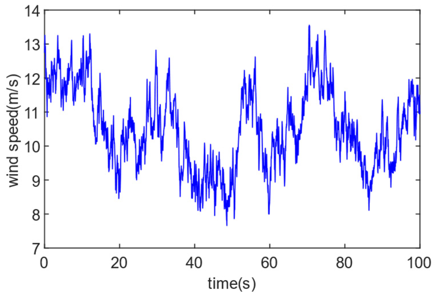
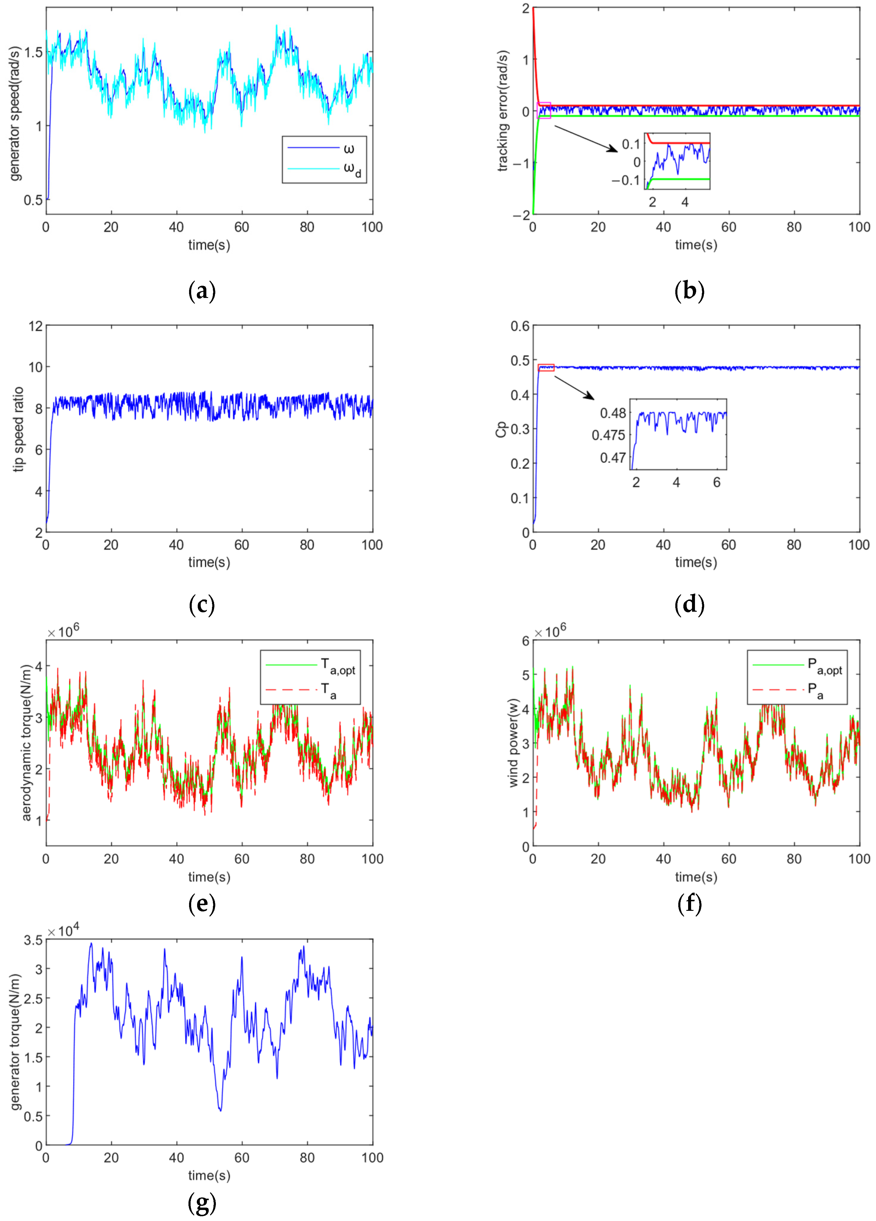
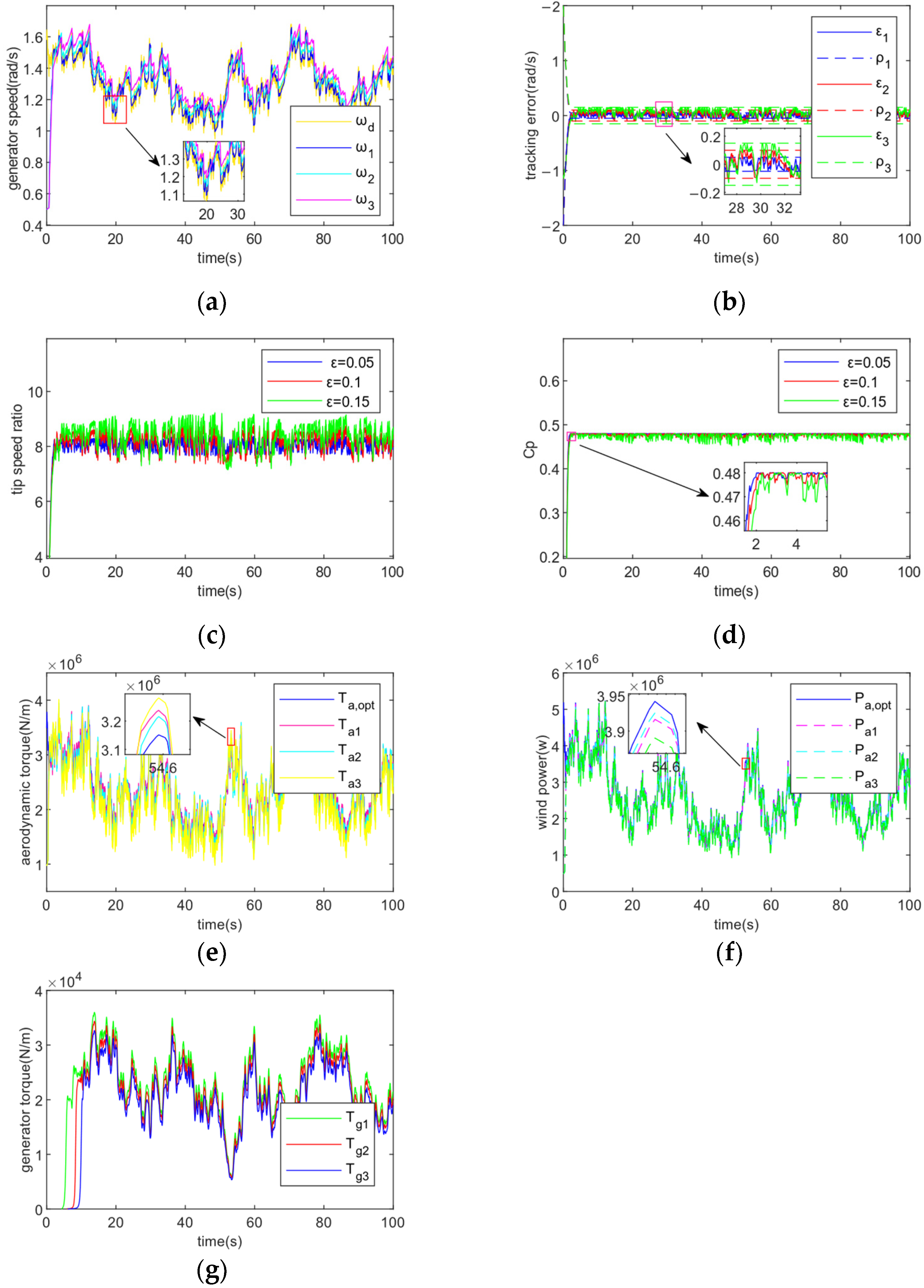
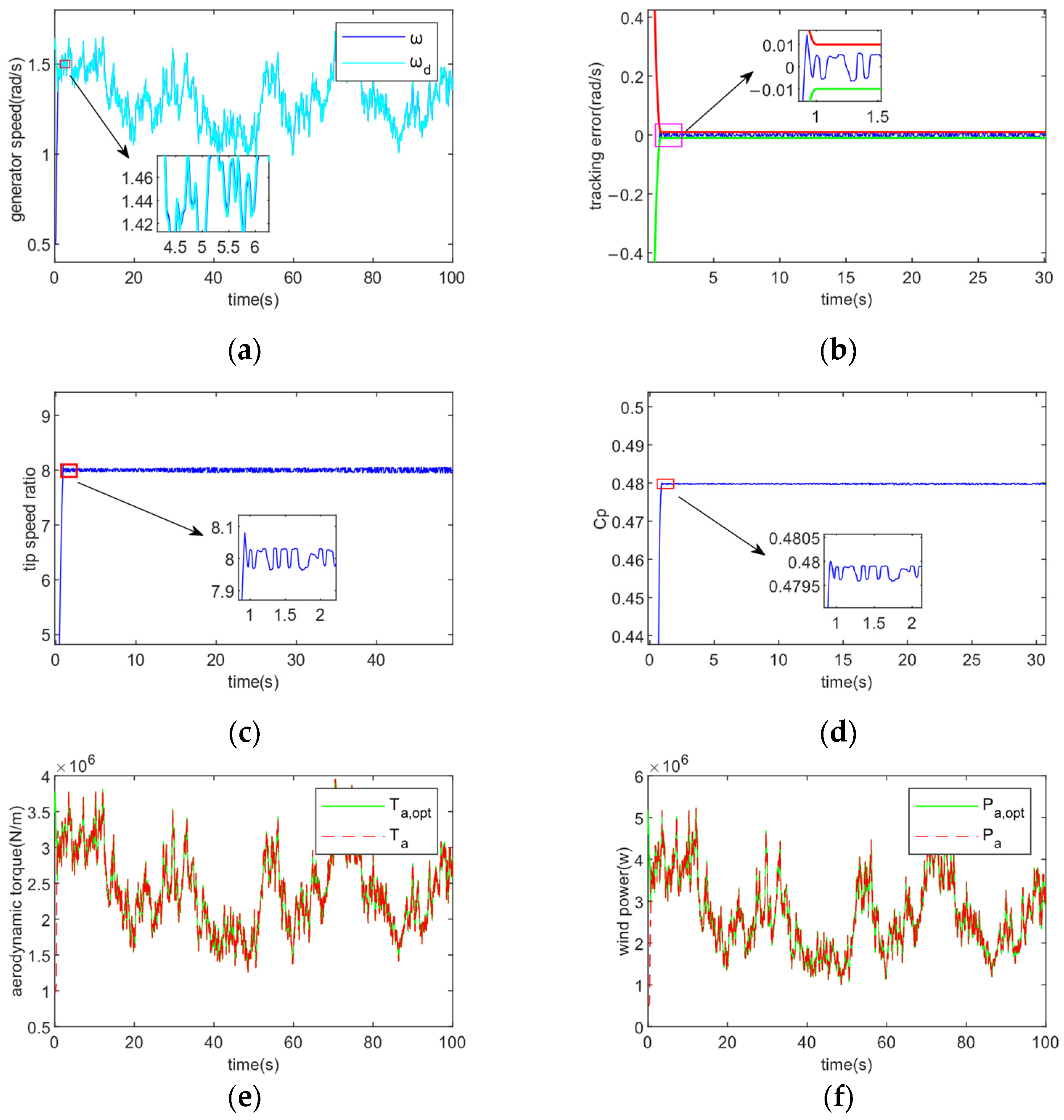
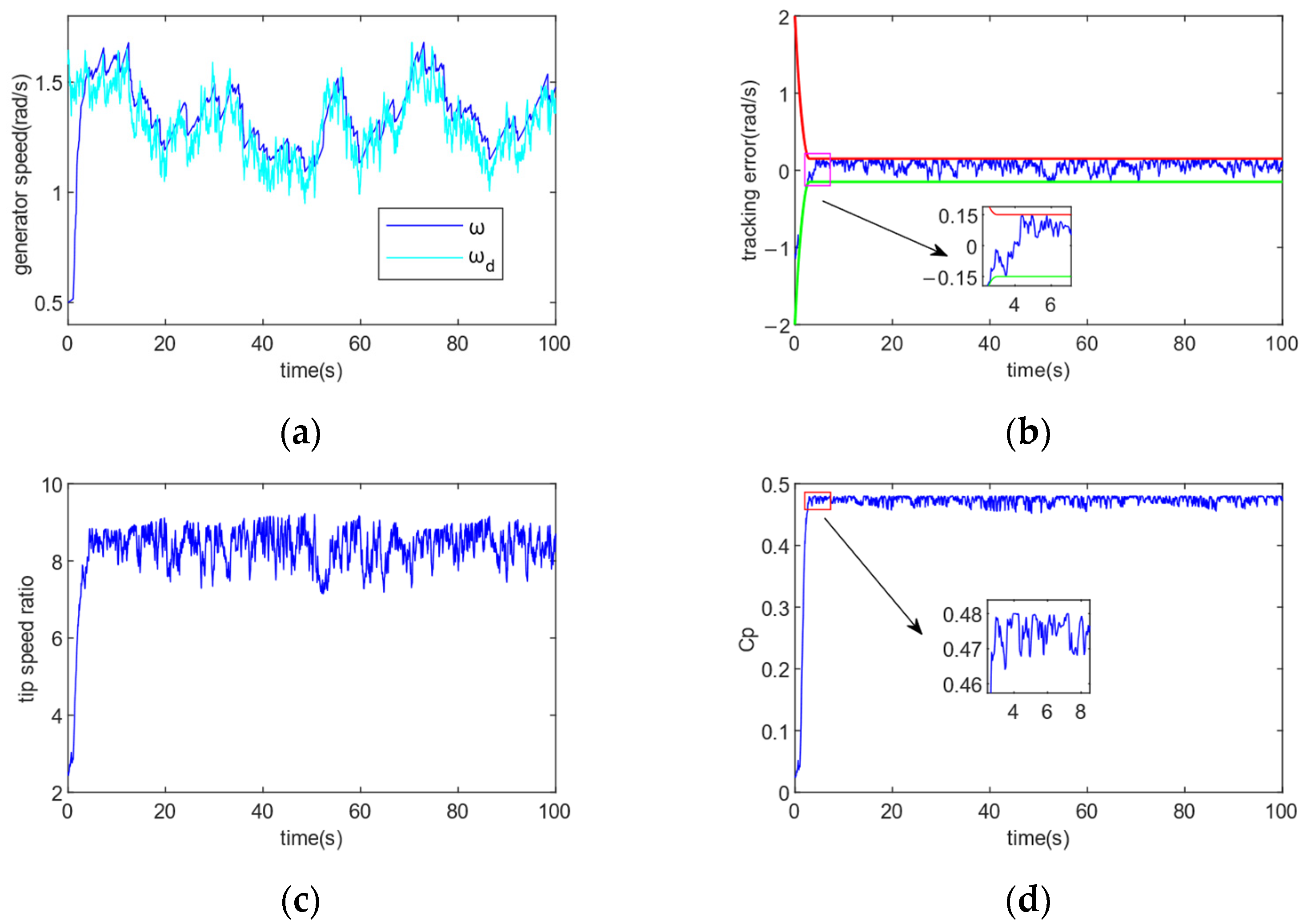
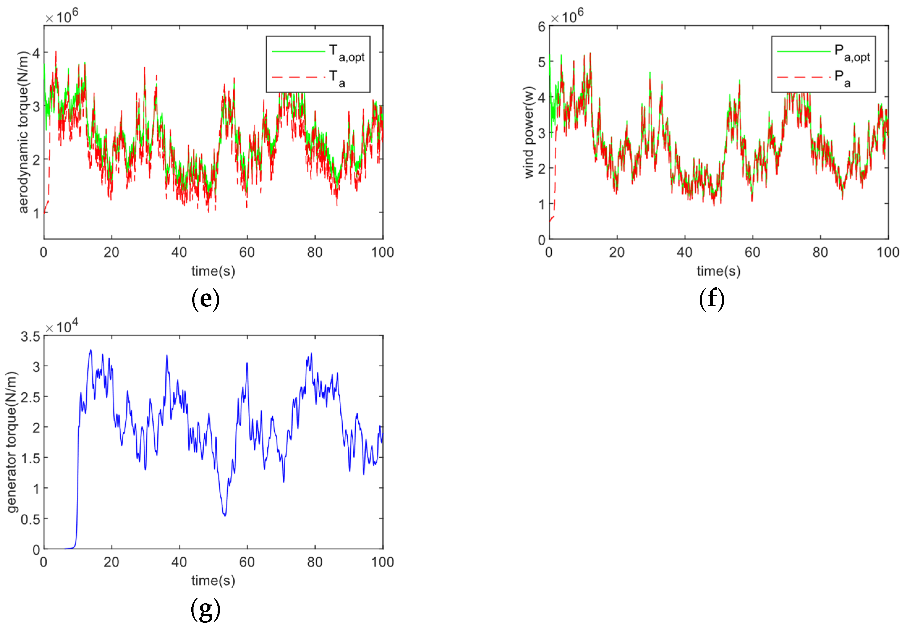
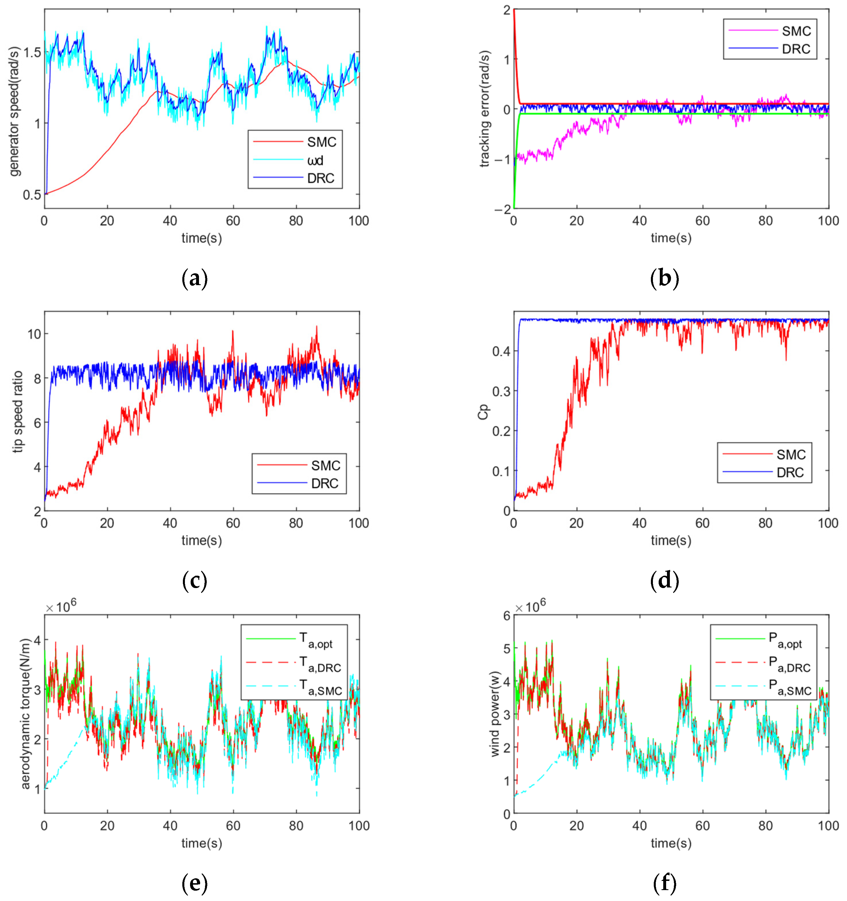
Proof of Theorem 1.

Consider the following Lyapunov function:

$$V=V_1+\cdots +V_n$$

(42)

By combining (28), (36) and (41), it follows that

$$\dot{V}\le -v{\displaystyle {\sum }_{i=1}^n{\overline{k}}_i{V}_i+v}{\displaystyle {\sum }_{i=1}^n{\Delta }_i\le -v\overline{k}}V+v\Delta$$

(43)

where $\overline{k}=\min \left\{{\overline{k}}_i,i=1,\cdots ,n\right\}$, $\Delta ={\displaystyle {\sum }_{i=1}^n{\Delta }_i}$.

To solve the above differential equation, we have:

$$V\le {\exp }^{-\overline{k}{\displaystyle {\int }_0^{t}v\left(s\right)ds}}V\left(0\right)+\Delta {\displaystyle {\int }_0^t{\exp }^{-\overline{k}{\displaystyle {\int }_{\tau }^{t}v\left(s\right)ds}}}v\left(\tau \right)d\tau$$

(44)

Using Lemma 2 in Section 2.2, we can get:

$$V\le {\exp }^{-\overline{k}{\displaystyle {\int }_0^{t}v\left(s\right)ds}}v\left(0\right)+\frac{\Delta }{\overline{k}}$$

(45)

We are now prepared to establish the following theorem’s conclusions.

Firstly, we show that objective $\left(\mathrm{a}\right)$ is achieved. Since we may deduce from (45) that $V\in L_{\infty }$ holds for every constrained beginning condition, it follows that $h_i\in L_{\infty }$, ${\varphi }_i\in L_{\infty }$. Thus, the closed-loop system is stable, the signals $h_i$ and ${\varphi }_i$ are ultimately uniformly bounded.

Next, we show that objective $\left(\mathrm{b}\right)$ is achieved. Since $h_i$ is bounded, we can derive $-\rho <w_i<\rho$ according to Lemma 3 in Section 2.3. The tracking error obeys the performance constraint $\left|w_i\left(t\right)\right|<\rho$ and converges to the specified region $\Omega =\left\{w_i\in ℝ,i=1,\dots ,n:\left|w_i\left(t\right)\right|<\epsilon \right\}$ within the predetermined time $T$, as shown by the fact that $\rho \left(t\right)$ as defined in Definition 2 of Section 2.2 will fall to $\epsilon$ within finite time $T$.

Finally, we show that objective $\left(\mathrm{c}\right)$ is achieved. Since $-\rho <w_i<\rho$, it follows that $w_i$ are constrained, which also suggests that ${\lambda }_i$ and ${\pi }_i$ are constrained. Note that $r_i$ is bounded, then it fellows from (9), (11), (13), (21), (30), (34) and (39) that the virtual controllers ${\partial }_i,{\overline{\partial }}_i,i=1,\dots ,n-1$ and actual controller $u$ are bounded. The proof is completed. □

4. Simulation Study

In this paper, Matlab (Version 9.12, R2022a) is used for simulation studies and Simulink (Version 10.5, R2022a) is used for controller design; the simulation model built is shown in Figure 5.

Table 1. Specific parameters of wind turbines.

Parameter Description	Value
Rated Power	5 MW
Rotor Radius	63 m
Gear Box Ratio	97
Cut-in Wind Speed	3 m/s
Cut-out Wind Speed	25 m/s
Rated Speed	1173.7 rpm
Rated Torque	43.093 KN∙m

displays the precise wind turbine specifications [29]. The simulation model includes wind speed disturbance uncertainty, and the control effect of the designed direct robust controller (DRC) is compared with that of the sliding mode controller (SMC) commonly used in maximum power tracking control. The turbulent wind model is produced using the Turbsim simulator, the use of which can be found in the OpenFAST|TurbSim User Manual. The resulting turbulent wind has an effective wind speed of 10 m/s and is used to simulate natural winds.

We now confirm that the suggested direct robust controller can provide the needed tracking precision $\left|e\left(t\right)\right|=\left|x\left(t\right)-y_d\left(t\right)\right|<0.1$ radians within the required time T = 2 s. The WT is first set up with $x\left(0\right)=0.5$ radians, since $x\left(0\right)-y_d\left(0\right)=0.5$, the prescribed performance functions is chosen as:

$$\rho =\{\begin{array}{l}{\left(\frac{T-t}{T}\right)}^2\left({\rho }_0-\epsilon \right)+\epsilon ,0\le t<T\\ \epsilon ,t\ge T\end{array}$$

(46)

where ${\rho }_0=2$, $\epsilon =0.1$, $T=2$. In simulation, the direct robust control algorithm (32) is utilized to deduce the control input $u$.

Figure 6 shows the turbulent winds with effective speed being 10 m/s. Figure 7 displays the controller’s tracking performance for tracking accuracy $\epsilon =0.1$ and convergence time $T=2$. In Figure 7, (a) shows that the control method achieves sensitive tracking of the generator speed $\omega$ against the optimal generator speed ${\omega }_d$ under random fluctuations in wind speed; (b) demonstrates that the tracking error achieves the control goal of error tracking by converging to the required accuracy range in the provided convergence period t = 2 s; (c) demonstrates how the tip speed ratio is kept to vary about the ideal value even after the tracking error has converged to the defined range; (d) demonstrates how the rotor power coefficient is maximized and the greatest amount of wind energy is captured by altering the tracking wind turbine’s ideal speed; (e) and (f) show that the control method enables fast tracking of its optimal trajectory by aerodynamic torque and wind power; (g) shows that the speed is varied by adjusting the generator torque to cope with wind speed variations. Fast tracking is accomplished via the control approach.

The impact of various controller settings on the system is then confirmed. The effect of convergence time $T$ on the system is first verified. Figure 8 shows the control performance of the controller for a fixed tracking accuracy $\epsilon =0.1$ and varying the controller convergence time $T$ to 1, 2, and 3 respectively. (a) shows that the magnitude of the convergence time $T$ affects how fast the wind turbine speed tracks to the desired speed trajectory; the smaller $T$, the faster the tracking speed, where ${\omega }_1$, ${\omega }_2$, and ${\omega }_3$ are the wind turbine speeds at convergence times $T$ = 1, 2, and 3, respectively, and ${\omega }_d$ stands for desired speed; (b) demonstrates how the size of the convergence time $T$ affects how quickly the tracking error converges to within a certain accuracy; the smaller the $T$, the quicker the convergence, where ${\epsilon }_1$, ${\epsilon }_2$, and ${\epsilon }_3$ correspond to convergence times $T$ of 1, 2, and 3 respectively; (c) and (d) show that the smaller the convergence time T, the shorter the time taken to reach the ideal blade tip speed ratio and the highest rotor power coefficient. Panels (e), (f) and (g) show that the smaller the convergence time $T$, the shorter the time to track the optimal aerodynamic torque and wind power trajectory, and the faster the generator torque is involved in the regulation process.

The system’s impact on tracking accuracy is then confirmed. Figure 9 demonstrates the control performance of the controller for fixed convergence time $T$ = 2 and varying the tracking accuracy $\epsilon$ of the controller to 0.05, 0.1 and 0.15 respectively. (a) shows that the magnitude of the tracking accuracy $\epsilon$ affects the sensitivity of the generator speed to the optimal generator speed trajectory tracking, the tracking is more sensitive and precise when $\epsilon$ is smaller, where ${\omega }_1$, ${\omega }_2$, and ${\omega }_3$ are the turbine speeds at tracking accuracy $\epsilon$ = 0.05, 0.1, and 0.15 respectively, and ${\omega }_d$ is the desired turbine speed; from (b) it is clear that the magnitude of the tracking accuracy $\epsilon$ affects the final convergence range of the tracking error, tracking accuracy is increased by decreasing the $\epsilon$, where the values of ${\epsilon }_1$, ${\epsilon }_2$, and ${\epsilon }_3$ are 0.05, 0.1, and 0.15, respectively, and ${\rho }_1$, ${\rho }_2$, and ${\rho }_3$ are the corresponding performance bounds at different tracking accuracies; (c) and (d) show the different fluctuations of the blade tip speed ratio and rotor power coefficient around the optimal value at different tracking accuracies, the larger the $\epsilon$, the greater the fluctuation amplitude, and vice versa, the flatter the fluctuation amplitude; (e) and (f) show that the smaller the tracking accuracy $\epsilon$, the higher the coincidence of optimal aerodynamic torque and wind power trajectory tracking, i.e., the higher the tracking accuracy; (g) shows how the smaller the tracking accuracy $\epsilon$, the more sensitive the regulation of the generator torque and the greater the regulation when the wind speed changes rapidly.

Next, we verify that preset performance tracking (PPT) can be achieved. We demonstrate that, given various beginning circumstances, the suggested controller can successfully perform PPT tracking. Figure 10 shows the tracking performance when $\epsilon =0.01$, $T=1$. In Figure 10, compared to Figure 7a, (a) shows that the generator speed $\omega$ tracks the ideal speed ${\omega }_d$ trajectory more sensitively after changing the initial conditions; the tracking error converges to a smaller error range more quickly, as seen in (b), improving the tracking accuracy; (c) and (d) show that after changing the initial conditions, the rotor power coefficient and tip speed ratio fluctuate less and stay close to their ideal levels; (e) and (f) show that the tracking sensitivity of the aerodynamic torque and wind power to their desired values becomes higher after changing the combination of controller parameters; (g) shows how the improved control accuracy results in a more rapid and sensitive adjustment of the generator torque to cope with rapid changes in wind speed. The control objective is achieved.

Subsequently, we varied the parameters of the controller so that $\epsilon =0.15$, $T=3$ to verify the effect of different parameter combinations on the performance of the controller. Figure 11 shows the tracking performance when $\epsilon =0.01$, $T=1$. Figure 11 compares with Figure 7 as well as Figure 10. The corresponding panel (a) show a decrease in the sensitivity of the turbine speed $\omega$ to the desired trajectory ${\omega }_d$ tracking and a decrease in trajectory coincidence after increasing the tracking accuracy and convergence time T. Panel (b) shows a slowdown in the convergence of the tracking error to within a given accuracy range, with a larger accuracy range leading to a decrease in control accuracy; panels (c) and (d) show controller parameter combinations show a significant increase in the fluctuation of the leaf tip speed ratio and rotor power coefficient around the optimum value. It can be seen that the selection of suitable controller parameters is crucial to improve the control effect; (e) and (f) show a reduction in sensitivity to optimal trajectory tracking of aerodynamic torque and wind power after increasing the convergence time $T$ and tracking accuracy $\epsilon$; (g) shows the slower and less regulated involvement of the generator torque in the regulation. Choosing the right controller parameters is crucial.

In this paper the controllers are selected as direct robust controllers and sliding mode controllers, and the simulation curves are compared. The SMC controllers used are as follows [30]:

First define a sliding surface:

$$s=\dot{e}+\lambda e=0;\lambda >0$$

(47)

Consider the following systems:

$$\ddot{y}=f(y)+u$$

(48)

where $y$ represents the system status, the control laws of the system are as follows

$$u=u_0=-f+\ddot{y}-\lambda \dot{e}$$

(49)

produces $\dot{s}=0$. For a zero starting condition, the system converges exponentially $s(t_0)$.

By introducing a discontinuous term as $KSgn(s)$ in the control $u_0$ for $K>0$, the system’s closed-loop dynamics are brought closer to a sliding surface. The system will arrive to the sliding surface in a limited amount of time at $s=0$. If a parametric estimate of $f$, $\widehat{f}$ is provided in the presence of uncertainties, the control rule changes to $\widehat{u}=KSgn(s)+u$. Thus there are:

$$u=-f+{\ddot{y}}_d-\lambda \dot{e}-KSgn(s)$$

(50)

This results in $\dot{s}=f-\widehat{f}-KSgn(s)$.

It is clear from Figure 12 that the DRC controller is more effective. (a) and (b) show that under the strong disturbance of external perturbation, the DRC control makes the tracking error converge quickly to the specified accuracy range, achieving sensitive tracking of the required speed trajectory and ensuring the best speed of the generator, while the tracking error under the SMC control gradually maintains stability after 35 s and the fluctuation amplitude exceeds the given accuracy range; (c) and (d) show that the DRC controller is able to track the TSR more accurately and quickly, and achieves the tracking of the optimal tip speed ratio within the preset time of 2 s, so that the rotor power coefficient reaches the maximum value to obtain the best wind power and achieve the control targets, while the SMC controller has a slower tracking speed and the control effect is unstable, and the TSR and C_p fluctuate more around the optimal value; (e) and (f) show that the DRC controller is more responsive to rapid changes in wind speed than the SMC controller, enabling maximum capture of wind energy by maximising aerodynamic torque and wind power within a pre-given time of T = 2 s.

5. Conclusions

In this study, a DRC control strategy for WT systems’ maximum power tracking is suggested. The control scheme can be pre-given arbitrary parameters and can make all tracking errors converge to within a specified accuracy range $\epsilon$ within a time $T$ given by the designer. Experiments prove that the size of the convergence time $T$ determines how fast the tracking error converges to within the given accuracy range; the smaller the $T$, the faster the speed. While the tracking accuracy $\epsilon$ determines the final convergence range of the tracking error, i.e., it affects the accuracy of the control, the smaller the $\epsilon$, the higher the control accuracy. Choosing the right tracking accuracy $\epsilon$ and convergence time $T$ can achieve sensitive tracking of the error. For wind turbine systems, the control scheme can track the optimal blade tip speed ratio for a given tracking accuracy and speed, and achieve fast and accurate tracking of the optimal turbine speed trajectory, e.g., within a convergence time $T=1\mathrm{s}$, so that the tracked speed error converges to an accuracy range of 0.01 for the upper and lower limits, and the rotor power coefficient reaches its maximum. Further, the tracking accuracy can be changed to reduce the fluctuation of wind energy utilization coefficient and TSR near the ideal value, with the goal to achieve the greatest power tracking control and the most wind energy collection, with strong robustness in the face of complex wind speed changes, and the control input is bounded and smooth. However, the wind turbine model is simplified for research, and a complicated non-linear wind turbine model will be incorporated in further work to confirm the controller’s effectiveness in terms of control.

References

1. Cao, Y.; Cao, J.; Song, Y. Practical prescribed time tracking control over infinite time interval involving mismatched uncertainties and non-vanishing disturbances. Automatica 2022, 136, 110050. [Google Scholar] [CrossRef]
2. Cheng, M.; Zhu, Y. The state of the art of wind energy conversion systems and technologies: A review. Energy Convers. Manag. 2014, 88, 332–347. [Google Scholar] [CrossRef]
3. Jin, F.; Ran, Q. Maximum Power Control of Wind Turbines with Practical Prescribed Time Stability Based on Wind Estimation. In Proceedings of the 2022 IEEE 6th Information Technology and Mechatronics Engineering Conference (ITOEC), Chongqing, China, 4–6 March 2022; pp. 1775–1778. [Google Scholar]
4. Yin, M.; Li, W.; Chung, C.Y.; Zhou, L.; Chen, Z.; Zou, Y. Optimal torque control based on effective tracking range for maximum power point tracking of wind turbines under varying wind conditions. IET Renew. Power Gener. 2017, 11, 501–510. [Google Scholar] [CrossRef]
5. Abdullah, M.A.; Yatim, A.; Tan, C.W. A study of maximum power point tracking algorithms for wind energy system. In Proceedings of the 2011 IEEE Conference on Clean Energy and Technology (CET), Kuala Lumpur, Malaysia, 27–29 June 2011; pp. 321–326. [Google Scholar]
6. Hu, L.; Xue, F.; Qin, Z.; Shi, J.; Qiao, W.; Yang, W.; Yang, T. Sliding mode extremum seeking control based on improved invasive weed optimization for MPPT in wind energy conversion system. Appl. Energy 2019, 248, 567–575. [Google Scholar] [CrossRef]
7. Song, D.; Yang, J.; Cai, Z.; Dong, M.; Su, M.; Wang, Y. Wind estimation with a non-standard extended Kalman filter and its application on maximum power extraction for variable speed wind turbines. Appl. Energy 2017, 190, 670–685. [Google Scholar] [CrossRef]
8. Tan, Y.; Wu, L. Neuro-adaptive practical prescribed-time control for pure-feedback nonlinear systems without accurate initial errors. Int. J. Adapt. Control Signal Process. 2023, 37, 915–933. [Google Scholar] [CrossRef]
9. Krishnamurthy, P.; Khorrami, F.; Krstic, M. Robust adaptive prescribed-time stabilization via output feedback for uncertain nonlinear strict-feedback-like systems. Eur. J. Control 2020, 55, 14–23. [Google Scholar] [CrossRef]
10. Krishnamurthy, P.; Khorrami, F.; Krstic, M. A dynamic high-gain design for prescribed-time regulation of nonlinear systems. Automatica 2020, 115, 108860. [Google Scholar] [CrossRef]
11. Song, Y.; Wang, Y.; Holloway, J.; Krstic, M. Time-varying feedback for regulation of normal-form nonlinear systems in prescribed finite time. Automatica 2017, 83, 243–251. [Google Scholar] [CrossRef]
12. Wang, Y.; Song, Y. A general approach to precise tracking of nonlinear systems subject to non-vanishing uncertainties. Automatica 2019, 106, 306–314. [Google Scholar] [CrossRef]
13. Chang, L.; Han, Q.-L.; Ge, X.; Zhang, C.; Zhang, X. On designing distributed prescribed finite-time observers for strict-feedback nonlinear systems. IEEE Trans. Cybern. 2019, 51, 4695–4706. [Google Scholar] [CrossRef]
14. Chen, X.; Zhang, X.; Zhang, C.; Chang, L. A time-varying high-gain approach to feedback regulation of uncertain time-varying nonholonomic systems. ISA Trans. 2020, 98, 110–122. [Google Scholar] [CrossRef]
15. Huang, J.; Wen, C.; Wang, W.; Song, Y.-D. Design of adaptive finite-time controllers for nonlinear uncertain systems based on given transient specifications. Automatica 2016, 69, 395–404. [Google Scholar] [CrossRef]
16. Li, H.; Zhao, S.; He, W.; Lu, R. Adaptive finite-time tracking control of full state constrained nonlinear systems with dead-zone. Automatica 2019, 100, 99–107. [Google Scholar] [CrossRef]
17. Li, K.; Tong, S. Fuzzy adaptive practical finite-time control for time delays nonlinear systems. Int. J. Fuzzy Syst. 2019, 21, 1013–1025. [Google Scholar] [CrossRef]
18. Mao, J.; Huang, S.; Xiang, Z. Adaptive practical finite-time stabilization for switched nonlinear systems in pure-feedback form. J. Frankl. Inst. 2017, 354, 3971–3994. [Google Scholar] [CrossRef]
19. Song, Y.; Huang, X.; Wen, C. Tracking control for a class of unknown nonsquare MIMO nonaffine systems: A deep-rooted information based robust adaptive approach. IEEE Trans. Autom. Control 2015, 61, 3227–3233. [Google Scholar] [CrossRef]
20. Sun, Z.-Y.; Xue, L.-R.; Zhang, K. A new approach to finite-time adaptive stabilization of high-order uncertain nonlinear system. Automatica 2015, 58, 60–66. [Google Scholar] [CrossRef]
21. Wang, F.; Chen, B.; Liu, X.; Lin, C. Finite-time adaptive fuzzy tracking control design for nonlinear systems. IEEE Trans. Fuzzy Syst. 2017, 26, 1207–1216. [Google Scholar] [CrossRef]
22. Zhang, C.H.; Yang, G.H. Event-triggered practical finite-time output feedback stabilization of a class of uncertain nonlinear systems. Int. J. Robust Nonlinear Control 2019, 29, 3078–3092. [Google Scholar] [CrossRef]
23. Zhang, Z.; Wu, Y. Fixed-time regulation control of uncertain nonholonomic systems and its applications. Int. J. Control 2017, 90, 1327–1344. [Google Scholar] [CrossRef]
24. Yang, J.; Jie, W.U.; Yue, H.U. Backstepping method and its applications to nonlinear robust control. Control Decis. 2002, 17, 641–647. [Google Scholar]
25. Zhao, K.; Song, Y.; Wang, Y. Regular error feedback based adaptive practical prescribed time tracking control of normal-form nonaffine systems. J. Frankl. Inst. 2019, 356, 2759–2779. [Google Scholar] [CrossRef]
26. Bu, X.; He, G.; Wei, D. A new prescribed performance control approach for uncertain nonlinear dynamic systems via back-stepping. J. Frankl. Inst. 2018, 355, 8510–8536. [Google Scholar] [CrossRef]
27. Abdellatif, W.S.; Hamada, A.; Abdelwahab, S.A.M. Wind speed estimation MPPT technique of DFIG-based wind turbines theoretical and experimental investigation. Electr. Eng. 2021, 103, 2769–2781. [Google Scholar] [CrossRef]
28. Kamarudin, M.N.; Husain, A.R.; Ahmad, M.N. Control of uncertain nonlinear systems using mixed nonlinear damping function and backstepping techniques. In Proceedings of the 2012 IEEE International Conference on Control System, Computing and Engineering, Penang, Malaysia, 23–25 November 2012; pp. 105–109. [Google Scholar]
29. Shanzhi, L.I.; Wang, H.; Tian, Y.; Aitouche, A. A RBF Neural Network based MPPT Method for Variable Speed Wind Turbine System—ScienceDirect. IFAC-PapersOnLine 2015, 48, 244–250. [Google Scholar]
30. Gambhire, S.; Kishore, D.R.; Londhe, P.; Pawar, S. Review of sliding mode based control techniques for control system applications. Int. J. Dyn. Control 2021, 9, 363–378. [Google Scholar] [CrossRef]
Figure 1. Speed-torque curve of wind turbine.
Energies 16 04022 g001
Figure 2. Schematic diagram of the wind turbine structure.
Energies 16 04022 g002
Figure 3. Transmission system model.
Energies 16 04022 g003
Figure 4. Diagram of the controller.
Energies 16 04022 g004
Figure 5. Simulation system construction diagram.
Energies 16 04022 g005
Figure 6. Turbulent wind speed.
Energies 16 04022 g006
Figure 7. Tracking performance under ε = 0.1, T = 2. (a) Generator speed; (b) Tracking error; (c) Tip speed ratio; (d) Rotor power coefficient; (e) Aerodynamic torque; (f) Wind power; (g) Generator torque.
Energies 16 04022 g007
Figure 8. Tracking performance at fixed ε = 0.1, T for 1, 2, and 3 respectively. (a) Generator speed; (b) Tracking error; (c) Tip speed ratio; (d) Rotor power coefficient; (e) Aerodynamic torque; (f) Wind power; (g) Generator torque.
Energies 16 04022 g008
Figure 9. Tracking performance at fixed T = 1, ε 0.05, 0.1, and 0.15 respectively. (a) Generator speed; (b) Tracking error; (c) Tip speed ratio; (d) Rotor power coefficient; (e) Aerodynamic torque; (f) Wind power; (g) Generator torque.
Energies 16 04022 g009
Figure 10. Tracking performance under ε = 0.01, T = 1. (a) Generator speed; (b) Tracking error; (c) Tip speed ratio; (d) Rotor power coefficient; (e) Aerodynamic torque; (f) Wind power; (g) Generator torque.
Energies 16 04022 g010aEnergies 16 04022 g010b
Figure 11. Tracking performance under ε = 0.15, T = 3. (a) Generator speed; (b) Tracking error; (c) Tip speed ratio; (d) Rotor power coefficient; (e) Aerodynamic torque; (f) Wind power; (g) Generator torque.
Energies 16 04022 g011aEnergies 16 04022 g011b
Figure 12. Comparison of the control effects of different controllers for ε = 0.1, T = 2. (a) Generator speed; (b) Tracking error; (c) Tip speed ratio; (d) Rotor power coefficient; (e) Aerodynamic torque; (f) Wind power.
Energies 16 04022 g012