Abstract
Uniaxial trackers are widely employed as the frame for solar photovoltaic (PV) panel installation. However, when used in sloping terrain scenarios such as mountain and hill regions, it is essential to apply a solar-tracking strategy with the sloping factors considered, to eliminate the shading effects between arrays and reduce the electricity production loss due to terrain changes. Based on a uniaxial tracker on the sloping terrain of a PV farm located in Ningxia, this study established a uniaxial solar-tracking strategy for sloping terrain by integrating a spatial projection model with a dynamic shadow assessment method. In the proposed strategy, the optimal tilt angle of the PV array and related desirable adjustment are identified taking into consideration major parameters such as the shadow area ratio S and the average solar irradiance intensity G. A tool underpinned by Matlab Simulink has also been developed to realize the proposed solar-tracking strategy. With the input of a simulated ramp signal β and the dynamically changed time parameters, the tracking angle of PV arrays over the simulated duration is accurately predicted, followed by a series of experimental validations conducted on the winter solstice and a typical sunny day (15 September). Moreover, the study also explored the terrain impacts on solar tracking by comparing the sloping terrain and flat terrain applications. The analytic and experimental results indicate that (a) the maximum value of the G(β) function could serve as the input to identify the optimal tracking angle; (b) the application of the flat terrain tracking (FTT) strategy in sloping terrain would result in a reduction of average solar irradiance intensity harvested by the PV arrays with varying degrees; (c) in the context of an east–west −7° sloping terrain, compared with the FTT strategy, the sloping terrain tracking (STT) strategy enabled anti-shading tracking, and then increased the daily PV electricity yield by 0.094 kWh/kWp, which is around 1.48% of the daily energy production; (d) given a measurement with annual scale, the STT strategy could cause a 1.26% increase in the energy harvesting with a flat uniaxial PV array on a −7° slope terrain, achieving an annual increase of 25.16 kWh/kWp. The experimental comparative analysis validated the precision of the proposed solar-tracking model, which has far-reaching significance for achieving automatic solar-tracking of PV modules, as well as improving the capacity and efficiency of PV systems.
1. Introduction
The ongoing global energy crisis and the climate change challenge have found wide applications for clean energy sufficiency and green economy, which are becoming key factors for countries worldwide with respect to overcoming the barriers of resource depletion and achieving sustainable development [1,2]. Among the diverse sources of clean energy, PV electricity has attracted considerable attention due to its outstanding economic returns, flexible modular design, benefit of downsizing and lower application threshold [3]. To improve the sufficiency in land use and promote the penetration of solar PV systems, innovative application models and scenarios such as “PV farms” [4], “PV lakes” [5,6] and “PV mountains” [7,8] have emerged rapidly in recent years, among which the mountain PV farms have shown the most significant growth.
However, the mainstream fixed arrays, which are widely used in current mountain PV farms, often suffer low efficiency in solar radiation harvesting and are sensitive to the shading between PV arrays, resulting in high solar energy loss [9]. Therefore, study on automatic solar trackers for PV arrays has attracted wide attention from both academia and industry communities [10]. In line with the system structure, automatic solar-tracking systems can be classified as uniaxial/single-axis tracking and dual-axis tracking. Despite the dual-axis tracking system being normally of higher efficiency, it is technically unfeasible for large-scale applications at the current stage due to its system complexity, higher energy consumption and maintenance costs. A literature review indicates that with the integration of intelligent solar-tracking tools and strategies, a horizontal single-axis tracker could also achieve an equivalent improvement by reducing shading between PV arrays and promote the harvesting of solar radiation, thereby resulting in an increase around 15~20% in PV electricity generation [11]. In addition, the effect of east–west horizontal single-axis tracking is found to be better than that in the north–south direction [12].
In recent years, a considerable number of studies have been conducted to promote the optimal control of PV uniaxial solar tracking, aiming to promote the harvesting of on-panel solar energy. Batayneh et al. proposed a discrete uniaxial tracking system which enabled solar tracking by changing three optimal angles with a per hour resolution. Through this, the system solar energy harvesting was increased by 91~94% [13]. Lee et al. developed a uniaxial solar-tracking strategy which can automatically control the PV panels’ rotation from east 50° to west 50° through recording and comparing the instantaneous energy generated with different angles applied. With completion of detection, the PV modular would then be rotated to a desirable angle to maximize the power output. Results show that the PV electricity yield could be increased by 3.4~8.3% [14].
The literature review also demonstrates that astronomical calculations and sensors are widely integrated in the current uniaxial PV systems to track the orientation of sunlight and maximize the energy production. However, the performance of photoelectric sensors is sensitive to reflections or scattering from surrounding obstacles, which might lead to measurement or even functional errors [15]. Moreover, in adverse weather conditions, the strong scattering caused by sunlight passing through clouds can also significantly increase the energy consumption of PV tracking systems. Therefore, tracking systems based on sensor monitoring are limited for automatic tracking with clear sky views and good weather conditions [16]. Based on their studies of PV performance on complex weather conditions, Kuttybay et al. claimed that time-based uniaxial tracking systems taking into consideration the sun’s daily path are approximately 4.2% more efficient than those sensors’ integrated tracking systems, as PV sensor tracking could not accurately identify the sun’s position on rainy days [17]. Carlos et al. conducted comparative studies on two types of solar-tracking strategies, tracking the maximum direct irradiance and tracking the optimal orientation for maximum total irradiance. Simulation results illustrate that in the regions below latitude 60°, the total daily solar harvesting efficiency with respect to tracking the optimal orientation strategy is slightly better; normally, an increase of less than 1.8% can be achieved [18].
Recent studies in mountainous PV system performance also indicate that the slope terrain is one of the major factors affecting energy production, especially for those uniaxial systems. Underpinned by their PV performance studies in southern Spain, Francisco et al. found that in non-south-facing slope terrain, the azimuth of the rotation axis of the uniaxial trackers needs to be adjusted to the same direction as the slope azimuth rather than zero, to maximize the PV energy generation [19]. Leung et al. studied the terrain loss of a horizontal single-axis solar-tracking system on a 4% southwest slope, and the results show that the standard inverse tracking had a terrain loss of 2%, while the application of the slope-aware inverse tracking strategy could eliminate the terrain loss successfully [20].
In light of the above, for a horizontal single-axis array on slope terrain, an east–west tracking system is technically feasible, and the astronomical calculation approach could be selected for maximum total irradiance tracking. The inverse tracking technology based on slope factor analysis can be integrated to reduce terrain losses and promote PV power generation. According to the existing studies, this research organically integrated a dynamic shading analysis model, a total solar irradiance model and a PV power generation assessment model to optimize the solar tracking for horizontal single-axis PV arrays on sloping terrains (referred to as the slope terrain tracking strategy hereafter). The shadow area ratio S and average irradiance intensity G are employed as the judgment criteria. Related Simulink models are established based on the derived mathematical formulas. The control of PV tracking is simulated by inputting a slope signal β, and then the S-β and G-β curves can be obtained, respectively, to calibrate the optimal tracking angle. By comparing the simulation and experimental results, the impact of shadow on PV energy output is analyzed, and the efficiency of the proposed sloping terrain tracking strategy is verified. The rest of this article is organized as follows: Section 2 introduces the modelling and formulation, followed by simulations with different scenarios included in Section 3; Section 4 presents comparative studies and discussions, and after that come the concluding remarks and future study recommendations in Section 5.
2. Modeling of Automatic Tracking for Horizontal Single-Axis PV Arrays on Sloping Terrain
2.1. Formulation of Solar Irradiance Intensity
In the horizontal single-axis axis tracking systems, the PV panel tilt angle is adjusted to maximize the overall irradiance harvesting, which is dependent on the real-time monitoring data and serials of pre-set control rules. However, the generic meteorological data commonly obtained from the current practices can only provide the measured irradiance intensities on the horizontal plane; therefore, they are insufficient with respect to identifying the desired tilt angle for PV panels to maximize the overall irradiance received. To overcome this barrier, this study developed a solar irradiance intensity model based on astronomical calculations, by integrating it with a numerical simulation analysis, to determine the desirable tilt angle for PV panels to enable the highest solar irradiation harvesting.
The overall solar irradiance intensity on the horizontal plane Ih is composed of direct irradiance intensity Ibh and diffuse irradiance intensity Idh [21], which can be expressed as:
where h is the solar altitude angle (°), m is the air mass coefficient which refers to the ratio of the actual path to the shortest path of solar radiation passing through the Earth’s atmosphere, P is the atmospheric transparency coefficient and I0 is the solar irradiance at the top of the vertical atmospheric boundary (W/m2).
The total solar irradiance on a tilted surface It is determined by the direct irradiance Ibt, diffuse irradiance Idt and reflected irradiance Irt. Given the tilt angle β and the azimuth angle γ (0° for true south, 90° for true west and −90° for true east) of the tilted surface, the total solar irradiance on the tilted surface can be calculated by converting the irradiance components on the horizontal plane [22], which then can be determined by:
In these equations, θ is the solar incidence angle (in degrees) on the inclined surface; φ denotes the local latitude (in degrees); γ represents the azimuth angle (in degrees) of the inclined surface; δ refers to the declination angle (in degrees); ω is the hour angle (in degrees); and ρ is the mean value of ground reflectance (with a default value of 0.2).
2.2. Shadow Modelling for the Horizontal Single-Axis Tracker
The data used for the model validation and case analysis of this article come from a solar farm located in Ningxia, China. Horizontal single-axis PV arrays with a uniform north–south orientation are used in this solar farm. The PV arrays track the solar by rotating round east–west to eliminate array shadings. Limited by the land use and array space, it is essential to adjust the tracking angle in a timely manner especially when the solar altitude is low, to avoid array shadings. In this study, the formation mechanism of shading between arrays is analyzed using a proposed spatial projection method, and a dynamic shading model is developed to support the shadow area calculation in the sloping terrain context.
2.2.1. Shadow Model on the Horizontal Plane
Given a uniaxial PV array placed on the horizontal plane, the generated shading between front and rear PV strings can be shown as in Figure 1. Suppose the longitudinal length of PV string is b, the width is a, the length of the shaded part of the PV panel is by, the width is ay and the shaded area is C. The horizontal spacing of the PV array is L, the inclination angle of the PV panel is β (positive facing west, negative facing east), the solar altitude angle is h, and the solar azimuth angle is α (with due south as 0°, positive westward and negative eastward). As demonstrated in the figure, the shading of the PV array would be affected by the position of the sun, as well as the array dimensions. The geometric relationship between the width of the shaded area and the width of the PV string, spacing and solar altitude angle can be presented as in Figure 1b,c. Thus, the shaded width ay can be determined via Equation (9).
where the solar azimuth angle α is the angle formed by the solar ray projection on the horizontal plane and the due south direction, as shown in Figure 1a. The shade length is only related to the magnitude of the solar azimuth. Thus, the shaded length by can be expressed as:
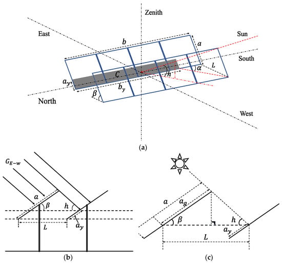
Figure 1.
Shading of PV strings on the horizontal ground: (a) Shading illustration, (b) Sideview of cross-section, (c) Geometric interactions.
Since solar rays are approximately a kind of parallel light source, according to the principle of parallel projection, it is known that given a plane is parallel to the projection plane, its projection will reflect the original shape. With the same tracking angle applied, uniaxial PV strings are parallel to each other; thus, the shape of the shaded area would be rectangular. Therefore, the shading area C on the horizontal plane is determined as:
2.2.2. Shadow Model on the Sloping Terrain
Despite the fact that changes in terrain factors might occur in arbitrary directions, the uniaxial arrays can eliminate the north–south terrain differences by adjusting the PV mounting angle to keep the axis horizontal. Therefore, on flat ground and sloping terrain, the difference in shading mainly comes from the elevation difference D between the front and rear PV strings in the east–west direction. Setting D = 0 on the flat ground as a reference, when the foundation of the rear row PV strings is higher, then D > 0. Therefore, sloping terrain can help to reduce shading. In contrast, when D < 0, the sloping terrain would exacerbate the shading between arrays. The slope angle i in the east–west direction can be used to represent the slope value, and its sign can be defined as i > 0 for a slope facing west, i < 0 when it faces east and i = 0° on flat ground. These data can be obtained from the on-field measurement.
As shown in Figure 2, the tilt angle of a PV array varies with the solar azimuth, which might reverse the front and rear arrays, resulting in a change in the sign of the elevation difference D. With the sign of the constant sloping angle i as a baseline, when the solar azimuth angle α < 0, the PV panel would face east, and the sign of D is opposite to that of i, while for α > 0, the PV panel faces west, and D has the same sign as i. By integrating the geometric relationship, the formula for D value can be obtained as:
where α > 0, ± takes a positive sign and α < 0, ± takes a negative sign.
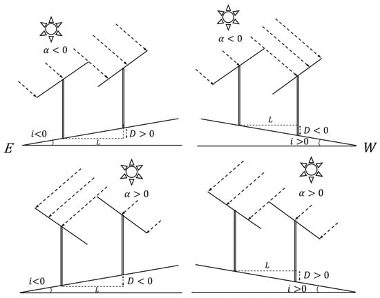
Figure 2.
Foundation height differences of PV arrays on the sloping terrain.
Figure 3a shows the shading of horizontal single-axis arrays for when the foundation height of the front array is lower than that of the rear array (D > 0). For a given position of the sun, the shading width of arrays on a sloping terrain would be reduced to ay′ (with a relative decrease amount of Δay) compared to the scenario of arrays on the horizontal ground. According to the geometric relationships shown in Figure 3b,c, the formula for the width of the shadow ay′ can be obtained from:
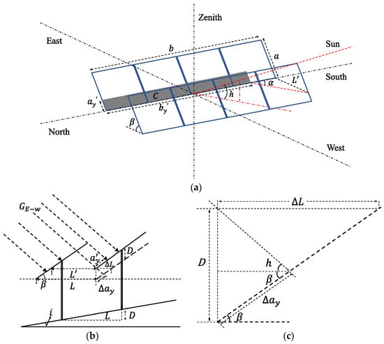
Figure 3.
Shading of PV strings on the sloping terrain: (a) Shading illustration, (b) Sideview of cross-section, (c) Geometric interactions.
As the width of the shadow area on the rear PV string ay′ is limited by the dimensions of the string, its value range should be [0, a], where ay′ < 0 means that the rear PV string would not be affected by the shadow; thus, ay′ can be set as 0. ay′ > a means the shadow width has exceeded the rear PV string, and ay′ needs to be set as a.
Due to the influence of slope topography, the horizontal spacing between the front and rear PV arrays would be reduced to L′ (with a relative reduction amount of ∆L), and the length of shadow blocking between arrays would be by′. Based on Equation (10), the formula for by′ calculation can be expressed as:
In Equation (16), 0 ≤ by′ ≤ b. Similarly, when by′ < 0, set by′ as 0; when by′ > b, set by′ as b.
According to the principle of the visual realism of parallel projection, it can be known that the shape of the shadow area between the horizontal single-axis arrays on the sloping terrain is still rectangular. Thus, the shadow blocking area can be determined by:
2.3. Horizontal Single-Axis Tracking Strategy for Sloping Terrain
The maximum on-panel solar irradiance can be obtained on the condition that the incident sunlight is aligned with the normal vector of the solar panel. Therefore, with the decrease in solar altitude, the tilt angle of the PV panel needs to be increased to reduce the angle formed by the panel normal vector and the incident sunlight, to maximize the on-panel solar irradiance. However, increasing the tilt angle would result in the growth of the shadow area between the arrays. Therefore, to determine the tracking angle for horizontal single-axis arrays, a model needs to be developed to reflect the interaction among the solar irradiance received by the array, the shadow area and the tilt angle of PV panels.
The ratio of the shadow area to the total area of PV array can be presented as the shadow area ratio S. When there is direct sunlight, the direct irradiance is much greater than the scattered and reflected ones; thus, the total irradiance at the shadow blockage point is much smaller than that at the unshaded point. Due to the significant difference in irradiance, the PV panel at the shadow blockage point would not work properly, and the solar irradiance at this point could be considered as complete loss. The average irradiance G received by the PV array can be calculated with Equation (19).
where the average radiation intensity G can be defined as the total solar radiation received by the unshaded part of the PV array. During the tracking process of a horizontal single-axis PV array, since the total PV panel area remains constant, the value of G varies with the amount of solar radiation received by the PV array. Therefore, the S-β and G-β curves obtained in this study can serve as a basis to identify the tracking angle for the horizontal single-axis PV array on sloping terrain. That is, under the condition of S = 0, the optimal tracking angle β is the one that could maximize the value of G.
2.4. PV Power Output Model
Figure 4 shows the equivalent circuit of a PV cell, which consists of an equivalent current source, a diode and a shunt resistance Rsh connected in parallel, and then connected in series with a resistance Rs. In this circuit, the photocurrent Iph from the current source flows out in three directions, the forward current Id of the diode, the shunt resistance current Ish, and the output current I flows through the series resistance Rs to the load [23].
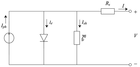
Figure 4.
Equivalent circuit of the PV module.
According to this equivalent circuit, the mathematic model of PV power output can be described as [24]:
In this equation, Np is the number of PV cells connected in parallel, while Ns represents the number of PV cells connected in series, Ir denotes reverse saturation current, Rs is the equivalent series resistance (Ω) of the load, Rsh is the equivalent parallel resistance (Ω) of the load, V is the output voltage (V), T refers to the PV module temperature (K), q represents electron charge (C), n is the diode ideality factor, and K is the Boltzmann constant. The photocurrent Iph is affected by the irradiance received by the PV module, which can be formulated as:
where Isc represents the short-circuit current (A), ki is the temperature coefficient of the photocurrent and Tn refers to the reference temperature (with a default value of 298 K).
In the simulation operations, the average irradiance intensity G of the entire array are assessed, then the photocurrent of PV cells is obtained by substituting the G-value into Equation (21). After that, the Iph is substituted into Equation (20) to obtain the theoretical I–V characteristic curve and output power of the PV module. Finally, the experimental data are compared and analyzed.
3. Simulation of a Flat Uniaxial Tracking Strategy on Sloping Terrain
3.1. Site Characteristic Parameters
On-site experiments were conducted in this study to validate the proposed solar-tracking strategy and models were developed using a horizontal single-axis PV array at a solar farm located in Ningxia, China. The current solar-tracking strategy for PV arrays was to ensure no shading between the arrays from 9 am to 3 pm on the winter solstice. Field measurements indicated that the ground coverage ratio (GCR) of the array on both flat and sloped terrains at this solar farm is 40%, and the essential parameters are shown in Table 1.

Table 1.
Key parameters of PV arrays.
The solar farm adopts horizontal uniaxial PV arrays that track in the north–south and east–west directions. The PV module is SPICM6(MAR)-72-365/PR, which was manufactured by the State Power Investment Corporation Xi’an Solar Power Co., Ltd. (Beijing, China). The main parameters of the PV modules are listed in Table 2.
Table 2.
Key Parameters of PV Modules.
3.2. Development of Simulation Modules
Based on the astronomical calculation formula and the mathematical model developed in this study, a Matlab/Simulink model was created to calculate the solar irradiance, dynamic shadow area and PV module output power. Input and output parameters are set and encapsulated as shown in Appendix A, Figure A1 and Figure A2. The slope signal β varies within the range [−45°, +45°], which is consistent with the tracking angle range. By inputting parameters such as date, time and slope angle i, the dynamic S-β and G-β curves can be obtained, which change over time and are used to determine the tracking angle of the slope terrain single-axis array. When the calculated target tracking angle differs from the current tracking angle by more than 1°, the motor is activated for tilt correction. The process of calculating and adjusting the tracking angle of the single-axis tracker using this tracking strategy is shown in Figure 5, where the date and time point are dynamic.
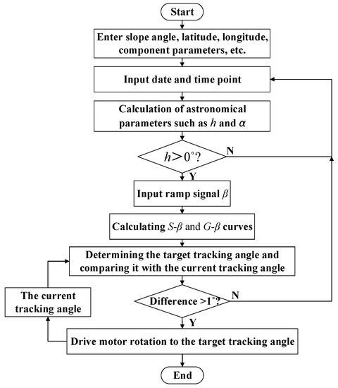
Figure 5.
Flowchart of the solar-tracking process.
3.3. Winter Solstice Typical Moments Simulation
As the solar farm is located in the Northern Hemisphere, the solar altitude angle on the winter solstice (22 December) is the lowest of the year. At this time, there might be shading and obstruction between the horizontal single-axis arrays. Therefore, the winter solstice is selected in this study as a typical day for simulations. The solar altitude and azimuth angles for each moment are shown in Figure 6. The corresponding parameters from Table 1 and Table 2 are involved as the inputs of the Simulink model, with the slope angle set as the typical slope of the solar farm (−7°). There are four typical moments on the winter solstice, including 15:30, 16:00, 16:30 and 17:00, selected for analysis.
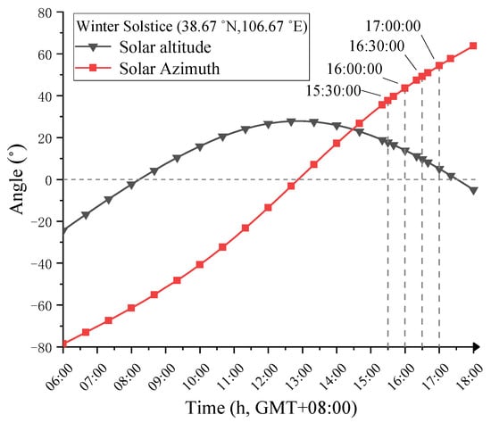
Figure 6.
Solar altitude and azimuth angles on the winter solstice.
The selected solar azimuth angles for the four time points are all greater than 0°. Therefore, the tracking range of the PV panel tilt angle β is from 0° to 45°. As shown in Figure 7, with a step size of 1°, S-β and G-β curves can be obtained by calculating the corresponding shadow area ratio S and the average irradiance G for each tilt angle β.

Figure 7.
Shadow area ratio and average solar irradiance variation curves.
According to the calculation results, when S = 0, the average irradiance intensity G might not obtain its maximum value; however, when G reached the maximum value, the corresponding tilt angle β would make S = 0, which aligns with the requirement of no shading between arrays and the maximum irradiance intensity received. Therefore, the optimal tracking angle βGmax can be obtained by solving for the maximum value of the function G(β).
3.4. Simulation Analysis of Different Sloping Terrains on the Winter Solstice
Given S(β) ≡ 0, the tracking angles of the horizontal single-axis arrays on different slopes would be the same. According to Equation (19), when S = 0, the average irradiance of the PV array G(β) equals the total irradiance on the tilted surface It(β); therefore, the optimal tracking angle β corresponds to the slope angle i where It is maximum. However, as shown in Equations (4)–(8), the calculation value of It is independent of the slope angle I; thus, the tracking angles of horizontal single-axis arrays on different slopes are the same.
To compare the tracking angles and average irradiance of horizontal single-axis PV arrays on different slopes, a Simulink numerical simulation was carried out at a typical time of 16:00 on the winter solstice day, with the range of slope parameters set to [−9°, +9°] and the step length set as 3°. The average solar irradiance G corresponding to each tilt angle β on seven typical slopes was obtained, and the G-β curves for each slope are demonstrated in Figure 8.

Figure 8.
Average irradiance curve of PV arrays on different slopes.
The following can be concluded from the simulation results: (1) On the −9° slope, the maximum average solar irradiance Gmax obtained by the PV array is 60.90% of that on the 9° slope, indicating that the slope topography factor has a significant impact on the irradiance that a fixed-axis array can receive at a given time. (2) Given a tracking strategy without consideration of the slope topography factors, according to the G-β curve on the 0° slope, it can be seen that the tracking angles on each slope are 23.5°. Compared with the βGmax on each slope, as the tracking angles of the array on −9°, −6° and −3° slopes are too large, the corresponding G values are reduced by 25.59%, 13.22% and 6.69%, respectively. The tracking angles of the array on 9°, 6° and 3° slopes are too small, resulting in a decrease in G values by 14.60%, 14.60% and 8.39%, respectively. (3) For a fixed-axis array on 6° and 9° slopes, S = 0 can be satisfied with any tracking angle β, since the G-β curve on the 6° slope coincides with that on the 9° slope.
To explore the impacts of slope topography on the tracking angle and average irradiance intensity of a horizontal single-axis solar tracker, a slope topography tracking strategy was established in this study. After that, numerical simulations were conducted based on the proposed strategy to identify the tracking angle βGmax and the average solar irradiance intensity Gmax considering seven typical slope scenarios on a winter solstice day. According to the solar altitude and azimuth angles presented in Figure 6, it can be seen that the power generation period on the winter solstice day mainly concentrates from 8:00 to 17:30. With a time step of 5 min, the βGmax and Gmax curves on each slope scenario can be obtained and shown as in Figure 9.
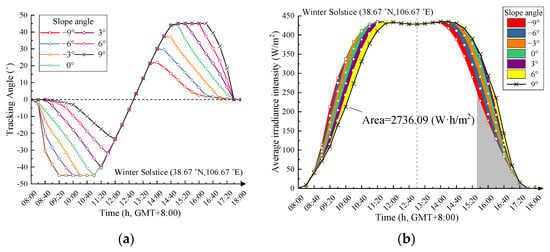
Figure 9.
Comparison of tracking angles and average irradiance intensity over slope terrains, (a) Tracking angles, (b) Average irradiance intensity.
As demonstrated in Figure 9a, compared to PV arrays installed on horizontal ground (i = 0°), the tracking angle of a uniaxial solar tracker on slopes was significantly affected by the sloping terrains especially in the morning and evening. Neglecting or underestimating the topographic factors would result in serious shading between PV arrays. In Figure 9b, the area enclosed by the average irradiance intensity curve and the X-axis represents the solar irradiance that a unit PV surface can receive. Taking i = 9° as the baseline, the area above the curve represents the positive irradiance, and vice versa. From 8:00 to 13:00, a smaller slope angle (which means the slope facing eastward) results in more irradiance received by the PV array. While from 13:00 to 18:00, a larger slope angle (which means the slope facing westward) would contribute more irradiance received by the PV array. By integrating the solar irradiance on various slopes and comparing it with that on the horizontal ground (i = 0°), the irradiance difference on different slope contexts then can be obtained and listed as in Table 3.
Table 3.
Solar irradiances under different sloping scenarios.
Despite the sloping tracking strategy being applied to adjust the tilt angle for the uniaxial array on sloped terrains, the solar irradiance harvesting in the slope scenarios remains lower than the peak harvesting with arrays installed on the horizontal ground. Moreover, the solar irradiation loss is proportional to the absolute value of the slope angle. Therefore, it can be concluded that the solar-tracking strategy can promote irradiation harvesting; however, it cannot eliminate the impacts of sloping topographies.
4. Comparative Study and On-Site Validation
4.1. Comparison of Simulation Results
To further explore the impacts of various tracking strategies on the solar energy harvesting efficiency of horizontal single-axis PV arrays on sloped terrains, both the simulation results and monitoring data on a typical sunny day (15th September) are collected for comparative studies in this project. Using the horizontal single-axis PV array (with −7° slope) in the solar farm, both the flat terrain uniaxial tracking (FTT) strategy and the sloping terrain uniaxial tracking (STT) strategy are applied in simulation analysis. The slope angle is employed as the control variable, with the slope angle of the FTT set as I = 0° and the slope angle of the STT set as I = −7° to match the real slope angle. All other variables and parameters remained the same. The FTT strategy is based on the astronomical formulas that track the maximum total irradiance and perform shadow avoidance, so it is equivalent to the standard tracking strategy for horizontal single-axis PV arrays on flat terrain, without consideration of sloping terrain.
Simulink simulation was performed with a step size of 2 min, and the uniaxial tracking angle data for both tracking strategies during the power generation period of 6:00–19:00 were obtained and are shown in Figure 10a. In order to investigate the differences in PV power output between the two tracking strategies and their causes, the differences in tracking angles between 16:30 and 16:50 were selected for analysis. According to Equation (19), the average irradiance collected by the uniaxial PV array at −7° slope with different tracking angles was calculated, and finally, the PV panel yield was assessed with the proposed PV model; the results are shown in Figure 10b.
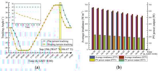
Figure 10.
Comparison of simulation results: (a) Tracking angles, and (b) Average irradiance and PV power output.
Results indicate that when compared to the FTT, the STT could significantly reduce the tracking angle of the uniaxial array over the studied period. Within the duration of 16:30 to 16:50, the STT promoted the harvesting of solar irradiance intensity by 2.67%, thereby enabling the average yield of PV arrays by 2.88%.
4.2. On-Site Validations
To further explore the impacts of tracking strategies on the efficiency of horizontal single-axis PV systems, on-site validations have been conducted in the solar farm located in Ningxia, China (as shown in Figure 10a). The PV arrays are installed in sloping terrain, and the parameter settings are aligned with those used in simulations. An experimental group and a control group were set up, and horizontal single-axis PV arrays on a 7° slope on 15 September (typical sunny day) were selected as the target objects. The tracking angles of the two groups of horizontal single-axis arrays were adjusted throughout the day in line with the STT and the FTT strategies, respectively.
Each group of horizontal single-axis PV arrays consists of 16 PV strings, and each string contains 27 monocrystalline silicon PV panels, with an installed capacity of 157.68 kWp. The shadow occlusion length and width of the PV strings were measured with 2 min intervals, then the shadow area ratio S between PV arrays was calculated. Monitoring power output and daily PV electricity yield were obtained from the inverter reading. The data collected within the period of 16:30 to 16:50 are presented in Figure 11.
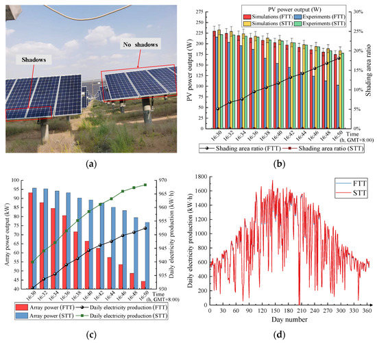
Figure 11.
Comparison of experimental results with the two tracking strategies: (a) FTT (left) and STT (right) at 16:30, (b) Shading area ratio and PV power output, (c) Monitoring array power output and daily electricity production and (d) Comparison of the array’s annual electricity yield.
As shown in Figure 11a,b, shading occurs between the horizontal single-axis arrays that adopt the FTT strategy; however, there is no shading occlusion in the PV arrays using the STT strategy over the entire monitoring period. Based on the on-site results of a typical sunny day with −7° slope terrain, by adjusting the tracking angle obtained from the STT strategy, the horizontal single-axis arrays could achieve shading-avoidance tracking.
In Figure 11b, the power output data of the studied PV panels obtained from both simulations and experiments are compared. For the horizontal single-axis arrays using STT, the error between the simulated and monitoring data in PV output is less than 5%. Therefore, the STT simulation model possesses higher degree alignment with the experimental results, with a maximum error of less than 5%. For the FTT, the larger shading occlusion area between arrays often means greater deviation between monitoring and simulated data in power output. As this deviation is less than 5% without shading occlusion, it can be concluded that the deviation resulted from the shading occlusion.
Except for the on-panel loss of solar radiation, shading is also the major contributor to the “hot spot effects”, which would consume the electricity generated by the PV cells as a load [25,26], resulting in a decrease in PV power output. Therefore, in the process of horizontal single-axis tracking, it is important to reduce the shading between arrays, which would correspondingly increase the PV power output, as well as extend the lifespan of PV components.
As shown in Figure 11c, compared to the FTT strategy, the STT strategy can significantly increase the average power output of PV arrays (up to 22.58%) during the period from 16:30 to 16:50. Comparative study of the simulation and experimental results could further identify the “hot spot effect” as the main contributor to the 19.7% power output loss of the FTT arrays.
The daily PV electricity generation of the experimental group and the control group measured at 19:00 were 1010.66 kWh and 995.93 kWh, respectively. Compared with the FTT, the STT strategy enabled a growth in daily energy harvesting by 1.48% (based on the horizontal single-axis array installed on a −7° slope), and the daily power generation per unit installed capacity was increased by 0.094 kWh/kWp. However, as the solar radiation intensity during the periods from 6:30 to 8:30 and 16:20 to 19:00 is relatively low, the growth of daily energy yield is relatively insignificant.
Figure 11d demonstrates the results of a comparative study; given the experimental results of a typical sunny day and supported by further simulation analysis, according to the weather conditions and annual power generation of the PV array in 2021, it is reasonable to expect that using the STT strategy could contribute an annual energy harvesting increase of 1.26% to the flat uniaxial array located on the −7° sloping terrain, resulting in an increase in the unit installed capacity of 25.16 kWh/kWp annually.
5. Concluding Remarks
Similar to the inverse tracking technology used in the solar tracking for the horizontal single-axis arrays, shading is prone to occur between PV arrays when the sun is at a low altitude, namely in the morning and evening. In these scenarios, shadow avoidance realized by applying tracking strategies is of great importance to improve the PV electricity yield and extend the lifespan of modules, particularly for those horizontal single-axis PV arrays installed on sloping terrains. In this study, a mathematical model was developed underpinned by a spatial projection method to identify the shadow area dynamically for the horizontal single-axis PV arrays installed on sloping terrains. The tracking angle at S = 0 is obtained from the S-β curve generated via the proposed model. Meanwhile, the tracking angle relative to the maximum average irradiance can be obtained from the G-β curve. Simulation results show that the related optimal tracking angle βGmax can be obtained by solving the maximum value of the G(β) function, which then can be used in the automatic solar tracking of the PV arrays.
Case studies indicate that to increase the on-panel irradiance received by PV arrays and thereby increase the power output of the system, when the PV arrays are installed on sloping terrains, the array spacing needs to be adjusted to avoid shading. Similarly, when the horizontal single-axis tracking is applied on sloping terrains, the tracking strategy also needs to be modified accordingly. This is confirmed by the validated simulations, showing that the application of FTT strategies on sloping terrain could result in tracking angles that are either too small or too large relative to βGmax on various sloping terrains, leading to a decrease in the harvesting of average solar irradiance and thus reducing the energy production of PV systems.
Experimental results on a typical sunny day (September 15th) with a −7° slope installation indicate that compared to the FTT strategy, the uniaxial arrays boosted via STT completely avoided shading between arrays, resulting in a 0.094 kWh/kWp increase in daily PV electricity generation, accounting for around 1.48% of the cumulative power output. Further simulations also indicate that the STT could contribute to an annual increase of 25.16 kWh energy production for each kWp PV installed on the −7° sloping terrain, which is around 1.26% promotion annually. Due to the site and time limits, this study is preliminarily focused on the analysis of horizontal single-axis arrays on an east–west −7° slope in a solar farm located in Ningxia, and a typical sunny day was selected to validate the efficiency improvement of PV electricity production achieved by the proposed slope tracking strategy. However, this automatic tracking strategy is also of technical feasibility and could be applied to different slope scenarios for year-round, all-weather analysis and tracking. Preliminary simulations indicate that the higher the latitude, the greater the increase in power generation of the sloping flat single-axis array after using the STT strategy. Due to the lower solar altitude angle at the same time in high latitude areas, arrays using the FTT strategy will experience larger shadowing areas. Therefore, by using the STT strategy to eliminate shading, a greater power generation improvement can be achieved. Future studies would be conducted via year-round, all-weather and multiple-scenario (by varying slope angles, geographic locations and array parameters) analyses to further improve the model accuracy and promote the overall power output of PV modules installed on sloping terrains.
Author Contributions
Conceptualization, B.H.; methodology, J.H.; validation, J.H. and M.X.; investigation, J.H. and L.L.; data curation, P.X. and W.Z.; writing—original draft preparation, B.H. and J.H.; writing—review and editing, K.X. and L.L.; visualization, P.X.; supervision, B.H. and K.X.; funding acquisition, B.H. and L.L. All authors have read and agreed to the published version of the manuscript.
Funding
This research was granted by the National Natural Science Foundation of China (Grant No. 51908064 and 52078060), Australia Cooperative Research Centre (CRC) for Low Carbon Living through the project ‘‘Integrated Carbon Metrics (ICM)” (RP2007), Changsha University of Science & Technology by the program ‘‘International Collaborative Research Underpinning Double-First-Class University Development” (2018IC19 and 2019IC17) and University of South Australia.
Data Availability Statement
The data presented in this study are available on request from the corresponding author. The data are not publicly available due to the contracts with the PV site.
Acknowledgments
We would like to thank Wuling Power Ningxia Branch and the Solar PV Farm for their support and assistance.
Conflicts of Interest
The authors declare no conflict of interest.
Appendix A

Figure A1.
Solar radiation intensity calculation model.

Figure A2.
PV power output simulation model.
References
- Brosemer, K.; Schelly, C.; Gagnon, V. The energy crises revealed by COVID: Intersections of Indigeneity, inequity, and health. Energy Res. Soc. Sci. 2020, 68, 5. [Google Scholar] [CrossRef] [PubMed]
- Wang, C.H.; Padmanabhan, P.; Huang, C.H. The impacts of the 1997 Asian financial crisis and the 2008 global financial crisis on renewable energy consumption and carbon dioxide emissions for developed and developing countries. Heliyon 2022, 8, 12. [Google Scholar] [CrossRef] [PubMed]
- Hill, C.A.; Such, M.C.; Chen, D.M. Battery Energy Storage for Enabling Integration of Distributed Solar Power Generation. IEEE Trans Smart Grid 2012, 3, 850–857. [Google Scholar] [CrossRef]
- Kim, J.H.; Hansora, D.; Sharma, P. Toward practical solar hydrogen production—an artificial photosynthetic leaf-to-farm challenge. Chem. Soc. Rev. 2019, 48, 1908–1971. [Google Scholar] [CrossRef]
- Hafeez, H.; Janjua, A.K.; Nisar, H. Techno-economic perspective of a floating solar PV deployment over urban lakes: A case study of NUST lake Islamabad. Sol. Energy 2022, 231, 355–364. [Google Scholar] [CrossRef]
- Perez, M.; Perez, R.; Ferguson, C.R. Deploying effectively dispatchable PV on reservoirs: Comparing floating PV to other renewable technologies. Sol. Energy 2018, 174, 837–847. [Google Scholar] [CrossRef]
- Sun, Q.Q.; Zhong, X.; Liu, J.Y. Three-dimensional modeling on lightning induced overvoltage for photovoltaic arrays installed on mountain. J. Clean. Prod. 2021, 288, 19. [Google Scholar] [CrossRef]
- Bellocchi, S.; De Iulio, R.; Guidi, G.; Manno, M.; Nastasi, B.; Noussan, M.; Prina, M.G.; Roberto, R. Analysis of smart energy system approach in local alpine regions—A case study in Northern Italy. Energy 2020, 202, 14. [Google Scholar] [CrossRef]
- Fathy, A. Reliable and efficient approach for mitigating the shading effect on photovoltaic module based on Modified Artificial Bee Colony algorithm. Renew Energy 2015, 81, 78–88. [Google Scholar] [CrossRef]
- Rahbar, K.; Eslami, S.; Pouladian-Karir, R. 3-D numerical simulation and experimental study of PV module self-cleaning based on dew formation and single axis tracking. Appl. Energy 2022, 316, 21. [Google Scholar] [CrossRef]
- Lazaroiu, G.C.; Longo, M.; Roscia, M.; Pagano, M. Comparative analysis of fixed and Sun tracking low power PV systems considering energy consumption. Energy Convers. Manag. 2015, 92, 143–148. [Google Scholar] [CrossRef]
- Nsengiyumva, W.; Chen, S.G.; Hu, L.H. Recent advancements and challenges in Solar Tracking Systems(STS):A review. Renew. Sustain. Energy Rev. 2018, 81, 250–279. [Google Scholar] [CrossRef]
- Batayneh, W.; Batainen, A.; Soliman, I. Investigation of a single-axis discrete solar tracking system for reduced actuations and maximum energy collection. Autom. Constr. 2019, 98, 102–109. [Google Scholar] [CrossRef]
- Lee, K.Y.; Chung, C.Y.; Huang, B.J. A novel algorithm for single-axis maximum power generation Sun trackers. Energy Convers. Manag. 2017, 149, 543–552. [Google Scholar] [CrossRef]
- Wang, Y.J.; Shi, Y.B.; Yu, X.Y. Intelligent Photovoltaic Systems by Combining the Improved Perturbation Method of Observation and Sun Location Tracking. PLoS ONE 2016, 11, e0156858. [Google Scholar] [CrossRef] [PubMed]
- Chowdhury, M.E.H.; Khandakar, A.; Hossain, B. A Low-Cost Closed-Loop Solar Tracking System Based on the Sun Position Algorithm. J. Sens. 2019, 2019, 3681031. [Google Scholar]
- Kuttybay, N.; Saymbetov, A.; Mekhilef, S. Optimized Single-Axis Schedule Solar Tracker in Different Weather Conditions. Energies 2020, 13, 5226. [Google Scholar] [CrossRef]
- Rodriguez-Gallegos, C.D.; Gandhi, O.; Panda, S.K. On the PV Tracker Performance: Tracking the Sun Versus Tracking the Best Orientation. IEEE J. Photovolt. 2020, 10, 1474–1480. [Google Scholar] [CrossRef]
- Gomez-Uceda, F.J.; Moreno-Garcia, I.M.; Jimenez-Martinez, J.M. Analysis of the Influence of Terrain Orientation on the Design of PV Facilities with Single-Axis Trackers. Appl. Sci. 2020, 10, 8531. [Google Scholar] [CrossRef]
- Liu, L.Q.; Han, X.Q.; Liu, C.X. The influence factors analysis of the best orientation relative to the sun for dual-axis sun tracking system. J. Vib. Control. 2015, 21, 328–334. [Google Scholar] [CrossRef]
- Housmans, C.; Ipe, A.; Bertrand, C. Tilt to horizontal global solar irradiance conversion: An evaluation at high tilt angles and different orientations. Renew. Energy 2017, 113, 1529–1538. [Google Scholar] [CrossRef]
- Jordehi, A.R. Parameter estimation of solar photovoltaic (PV) cells: A review. Renew. Sustain. Energy Rev. 2016, 61, 354–371. [Google Scholar] [CrossRef]
- Li, Z.; Ql, A.; Mc, A. A simplified mathematical model for power output predicting of Building Integrated Photovoltaic under partial shading conditions. Energy Convers. Manag. 2019, 180, 831–843. [Google Scholar]
- Zhang, F.; Wu, M.Y.; Hou, X.T. The analysis of parameter uncertainty on performance and reliability of photovoltaic cells. J. Power Sources 2021, 30, 507. [Google Scholar] [CrossRef]
- Ge, Q.; Li, Z.; Sun, Z. Low Resistance Hot-Spot Diagnosis and Suppression of Photovoltaic Module Based on I-U Characteristic Analysis. Energies 2022, 15, 3950. [Google Scholar] [CrossRef]
- Dhimish, M.; Holmes, V.; Mather, P. Novel hot spot mitigation technique to enhance photovoltaic solar panels output power performance. Sol. Energy Mater. Sol. Cells 2018, 179, 72–79. [Google Scholar] [CrossRef]
Disclaimer/Publisher’s Note: The statements, opinions and data contained in all publications are solely those of the individual author(s) and contributor(s) and not of MDPI and/or the editor(s). MDPI and/or the editor(s) disclaim responsibility for any injury to people or property resulting from any ideas, methods, instructions or products referred to in the content. |
© 2023 by the authors. Licensee MDPI, Basel, Switzerland. This article is an open access article distributed under the terms and conditions of the Creative Commons Attribution (CC BY) license (https://creativecommons.org/licenses/by/4.0/).