Optimizing Power Demand Side Response Strategy: A Study Based on Double Master–Slave Game Model of Multi-Objective Multi-Universe Optimization

Abstract

In the pilot provinces of China’s electricity spot market, power generation companies usually adopt the separate bidding mode, which leads to a low willingness of demand-side response and poor flexibility in the interaction mechanism between supply and demand. Based on the analysis of the demand response mechanism of the power day-ahead market with the participation of power sales companies, this paper abstracted the game process of the “power grid-sales company-users” tripartite competition in the electricity market environment into a two-layer (purchase layer/sales layer) game model and proposed a master–slave game equilibrium optimization strategy for the day-ahead power market under the two-layer game. The multi-objective multi-universe optimization algorithm was used to find the Pareto optimal solution of the game model, a comprehensive evaluation was constructed, and the optimal strategy of the demand response was determined considering the peak cutting and valley filling quantity of the power grid, the profit of the electricity retailers, the cost of the consumers, and the comfort degree. Examples are given to simulate the day-ahead electricity market participated in by the electricity retailers, analyze and compare the benefits of each market entity participating in the demand response, and verify the effectiveness of the proposed model.

1. Introduction

The new round of reform in the power sector has promoted the diversified development of market players, and the power demand-side response system has been gradually improved [1]. The electricity retailer has upgraded its revenue model from relying solely on price differentials to offering load integration and diversified comprehensive energy services. By balancing the varying demands of user groups and participating in demand-side response programs, the company not only actively cooperates with the peak-shaving and valley-filling measures of the power system but also increases its revenue. As the electricity market reform continues to deepen and the establishment of the electricity spot market gradually improves, the implementation model of demand response in the power sector is shifting from the “demand-side bidding + fixed compensation price” model to a market-oriented “demand-side bidding + maximum price limit” model [2,3]. The ability to optimize resource allocation by fully considering the demand side is crucial [4]. In this context, exploring the supply–demand interaction between the “grid–user–retailer” triad under market competition mechanisms and studying demand-side response strategies have become a pressing research topic.

Demand response subsidy pricing is an incentive measure established by grid companies to encourage consumers to reduce electricity consumption during peak periods, thereby reducing the burden on the power grid. Currently, there have been significant developments in the field of research related to demand-side resource prices [5] and the formulation of incentive mechanisms [6]. The traditional optimization theory system, which relies on single-agent decision-making, is unable to effectively address the challenges in actual power demand response management.Some artificial intelligence technology [7] and game theory methods [8] are applied to solve the power demand side response strategy [9]. Among them, there are two main types of applications for game theory: (1) The goal of studying demand-side electricity consumption behavior based on demand response optimized equipment is to discover the best strategy for arranging the power consumption of each device. Reference [10] presents a multi-layer game model that involves power companies, multiple home power management centers, and multiple devices within a household. This paper also proposed a response mechanism for managing household power load in a smart grid environment; (2) Investigate the game between the electricity demand side and the electricity supply company [11,12]. In reference [13], a game between electricity consumers and the power grid to determine the optimal price set by the grid, and users adjusting their optimal power consumption based on the price. Reference [14] thoroughly investigated decision-making behavior in power demand response management from the perspective of multi-population evolutionary game theory. At the same time, considering the master–slave game [15] very suitable for analyzing sequential decision-making problems in competitive environments [16], the basic theory of the modern engineering game has found extensive application in the domain of power system control and decision-making. Reference [17] tackles the issue of demand response subsidy pricing set by power grid companies. The research established a master–slave game model to illustrate the interaction between grid operators and multiple stakeholders. In reference [18], a master–slave game model was constructed with the aim of maximizing the interests of both users and load aggregator businesses. The optimal compensation pricing strategy for the load aggregator was obtained by solving the model, and the elasticity of user electricity consumption was analyzed to optimize user response. In the future, the demand response market will become more and more perfect, and the demand response model needs to consider the game of more market players.

In this paper, the response mechanism of the power market under the participation of retail electricity companies was analyzed, considering a more complete range of demand response participants in the market. With the goals of peak shaving and valley filling on the grid side, maximizing the profit of retail electricity companies and minimizing the electricity cost and ensuring the electricity comfort of users, the game process of “power grid-sales e-commerce-user” in the competitive environment of the power market was abstracted into a two-layer (power purchase layer/power sales layer) master–slave game model. After analyzing and solving the model, we proposed a new solution by introducing the multi-objective multiverse optimizer (MOMVO) algorithm [19]. This method converts the objective functions and constraints in the model into multiple fitness functions and seeks the Pareto front of the model. Finally, in the interactive game, by continuously interacting the respective benefit information between each subject, the Nash equilibrium solution that satisfies its own benefits is obtained, that is, the distribution of electricity and subsidy prices in which each market entity participates in demand response. By simulating the electricity market in which electricity sales companies participate, the benefits of demand response from various market entities were analyzed and compared, and the validity of the proposed model was confirmed.

2. Demand Response Revenue Model for Individual Market Players

In the event of power shortage (surplus) in the real-time balancing market, the power grid initiates a demand response mechanism for peak shaving (valley filling). Retail electricity companies participate in the demand response by purchasing electricity based on the electricity usage patterns of their customers, and then selling the electricity to them. This helps balance the demand and supply of electricity in the market. Upon receiving the incentive notification from the retail electricity company to reduce the load or the signal of rising electricity prices, the electricity users change their inherent electricity consumption patterns [20]. To guarantee the stability of the electricity network and regulate the increase of electricity costs, it is imperative to respond to power supply by reducing or shifting the electricity load during a specific time period. In response to the demand response programs issued by the grid, decisions are made by the demand side with the aim of maximizing the benefits of participation.

2.1. Demand Response Revenue Model for Grid

The benefits of the grid release of the peak-shaving demand response mainly include reduced power generation costs and avoidable transmission and distribution capacity costs; costs mainly include reduced electricity sales gains and compensatory costs for publishing demand responses.

(1) Reduced power generation costs:

$$C_f\left(Q\right)=a{Q}^2+bQ+c,$$

(1)

$$\mathrm{\Delta }{C}_f\left(Q\right)=C_f\left(Q\right)-C_f\left(Q^{\prime }\right),$$

(2)

where $a,b,c$ is the cost factor of power generation. Generally, $a>0$ and $2a$ represent the slope of the marginal cost price curve, b is the starting marginal cost of the unit, c is the loss when the unit does not contribute, Q is the amount of electricity generated before demand response, $Q^{\prime }$ is the amount of power generated after demand response, and $\mathrm{\Delta }{C}_f\left(Q\right)$ is the reduced power generation cost of the grid company.

(2) It can avoid transmission and distribution capacity costs.

The avoidable transmission and distribution capacity cost can be addressed through the avoidable transmission and distribution capacity per unit cost $c_g$ and the actual $\mathrm{\Delta }Q$ of avoided transmission and distribution capacity, as shown in Equation (3).

$$C_{con}=c_g·\mathrm{\Delta }Q.$$

(3)

Considering transmission and distribution losses, user participation in demand response does not directly correspond to load reduction on the grid side. The actual avoided transmission and distribution capacity $\mathrm{\Delta }Q$ can be calculated as follows:

$$\mathrm{\Delta }Q=\frac{1}{1-\alpha }.$$

(4)

Among them, $Q_t$ stands for the total response of users during the time interval t, and $\alpha$ denotes the coefficient of transmission and distribution losses in the grid.

(3) Publish demand response subsidy fees.

To incentivize retail electricity companies to participate in demand response, the grid provides them with a compensation price. The compensation cost $C_{r,g}$ can be calculated as follows:

$$C_{r,g}=\sum _{t=1}^T\sum _{k\in N}{r}_k^t{q}_k^t,k=1,2,\dots ,N,t=1,2,\dots ,T.$$

(5)

Here, T represents the set of time periods for demand response, N denotes the set of sales companies, $r_k^t$ is the subsidy unit price that the power grid provides to electricity retailer $k(k=1,2,\dots ,N)$ at period $t(t=1,2,\dots T)$, and $q_k^t$ refers to the response quantity of electricity retailer k during time period t.

(4) Reduced income from electricity sales.

$$B_{s,g}=\sum _{t=1}^T\sum _{k\in N}{q}_k^t{\lambda }_t,k=1,2,\dots ,N,t=1,2,\dots ,T.$$

(6)

Among them, $B_s,g$ denotes the reduction in electricity sales revenue for the power grid, $q_k^t$ is the response quantity of the electricity retailer k at time t, and ${\lambda }_t$ stands for the spot electricity price in the market at time t.

Equation (7) depicts the revenue function of the power grid when it engages in demand response.

$$U_G=C_{con}+\mathrm{\Delta }{C}_f-C_{r,g}-B_{s,g}.$$

(7)

2.2. Demand Response Revenue Model for Electricity Retailers

The cost of participating in pre-day peak shaving response of the grid is mainly comprised of reduced electricity sales revenue and allowance fees issued to users, while the income mainly consists of the response subsidies obtained.

(1) Demand response subsidies obtained.

The electricity retailer k participates in the day-ahead peak load reduction demand response program and receives subsidy payments, denoted by ${\overline{B}}_{r,k}$, as shown in Equation (8). Here, $r_k^t$ is the subsidy unit price received by electricity retailer k during time period t, and $q_k^t$ is the response amount of electricity sales company k during time period t.

$${\overline{B}}_{r,k}=\sum _{t=1}^T{r}_k^t{q}_k^t,k\in N,t=1,2,\dots ,T.$$

(8)

(2) Reduced power purchase costs.

The electricity retailer k participates in demand response and lowers the cost of procuring electricity from the grid, denoted by ${\overline{C}}_{g,k}$.

$${\overline{C}}_{g,k}=\sum _{t=1}^T{q}_k^t{\lambda }_k^t,k\in N,t=1,2,\dots ,T.$$

(9)

(3) Reduced electricity sales revenue.

This paper considered the signed time-of-use electricity pricing contract between the electricity sales company and users, where the electricity sales company determines the time-of-use periods and prices for the 24 h in a day in advance. The reduced electricity sales revenue ${\overline{R}}_{s,k}$ for the electricity sales company k is shown in Equation (10).

$${\overline{R}}_{s,k}=\sum _{t=1}^T\sum _{i\in M_k}{\tilde{q}}_i^t{\tilde{\lambda }}_k^t,k\in N,i\in M_k,t=1,2,\dots ,T.$$

(10)

Among them, ${\tilde{\lambda }}_k^t$ is the live electricity rate of the electricity retailer k corresponding to the user in the t period, $M_k$ represents the collection of users under the electricity sales company k, and ${\tilde{q}}_i^t$ is the response volume of the user $i(i=1,2,\dots ,M_k)$ during the t period.

(4) Published user response subsidy fees.

The subsidy price published by the electricity retailer to the user i during the t period is recorded as ${\tilde{r}}_i^t$, then the response subsidy fee ${\overline{D}}_{r,k}$ issued by electricity retailer k to user is shown in Formula (11).

$${\overline{D}}_{r,k}=\sum _{t=1}^T\sum _{i\in M_k}{\tilde{q}}_i^t{\tilde{r}}_i^t,k\in N,i\in M_k,t=1,2,\dots ,T.$$

(11)

(5) Penalty fees.

When the actual response amount of the users under the electricity retailer k is lower than 95% of the declared response amount or higher than 105% of the declared response amount by the electricity retailer, the penalty fee ${\overline{F}}_{\omega ,k}$ will be as shown in Formula (12), where ${\omega }_k$ is the penalty price of the electricity retailer k.

$${\overline{F}}_{\omega ,k}=\left\{\begin{array}{c}\hfill (q_k^t·95\%-\sum _{i\in M_k}{\tilde{q}}_i^t)·{\omega }_k,\sum _{i\in M_k}{\tilde{q}}_i^t<q_k^t·95\%,\\ \hfill (\sum _{i\in M_k}{\tilde{q}}_i^t-q_k^t·105\%)·{\omega }_k,\sum _{i\in M_k}{\tilde{q}}_i^t>q_k^t·105\%,\end{array}\right.k\in N,i\in M_k,t=1,2,\dots T.$$

(12)

The income of the electricity sales company k participating in the demand response ${\overline{U}}_{S,k}$ is as in Equation (13):

$${\overline{U}}_{S,k}={\overline{B}}_{r,k}+{\overline{C}}_{g,k}-{\overline{R}}_{s,k}-{\overline{D}}_{r,k}-{\overline{F}}_{\omega ,k},k\in N.$$

(13)

2.3. User Demand Response Revenue Model

(1) Response costs.

The cost of user response refers to the losses incurred by users reducing electricity consumption. In this paper, the user response cost ${\tilde{C}}_{q,i}$ is expressed as a quadratic function, as shown in Equation (14).

$${\tilde{C}}_{q,i}={\beta }_i{\left({\overline{q}}_i\right)}^2+\gamma {\overline{q}}_i,i\in M$$

(14)

$${\overline{q}}_i=\sum _{t=1}^T{\tilde{q}}_i^t,i\in M,t=1,2,\dots ,T,$$

(15)

where ${\beta }_i$ and ${\gamma }_i$ are the user i response cost factors, both constants greater than 0, and the response amount of the user is recorded as ${\overline{q}}_i$.

(2) Response subsidy fees received by users.

The subsidy price that user i receives during the t session is ${\tilde{r}}_i^t$, and the response subsidy fee that user i receives is ${\tilde{B}}_{dr,i}$.

$${\tilde{B}}_{dr,i}=\sum _{t=1}^T{\tilde{r}}_i^t{\tilde{q}}_i^t,i\in M,t=1,2,\dots ,T.$$

(16)

(3) Reduced power purchase costs.

In peak periods, users have the option to engage in demand response by either decreasing their consumption or shifting their usage, meaning that the demand response quantity of users includes both load reduction and load transfer.

Among them, the load transfer quantity for demand response scheduling by the user is mainly based on the demand elasticity theory. According to the demand principle of economics, the elasticity coefficient of electricity price may be characterized as the proportionate alteration in load demand resulting from the proportionate alteration in electricity price over a certain period, and the price elasticity coefficients are represented by Equation (17).

$$\left\{\begin{array}{cc}\hfill e^{t_1,t_2}& =\frac{\mathrm{\Delta }{L}_{t_1}/L_{t_1}^0}{\mathrm{\Delta }{P}_{t_2}/P_{t_2}^0}\hfill \\ \hfill e^{t_1,t_2}& \le 0,t_1=t_2;e^{t_1,t_2}\ge 0,t_1\hfill & \hfill \ne t_2.\end{array}\right.$$

(17)

Among them, $L_{t_1}^0$, $\mathrm{\Delta }{L}_{t_1}$ are the initial electricity load at the user’s $t_1$ moment and the load change before and after demand response, respectively. $P_{t_2}^0$, $\mathrm{\Delta }{P}_{t_2}$ are the initial electricity price at $t_2$ and the price change before and after demand response, respectively. When $t_1=t_2$, $e^{t_1,t_2}$ is called the self-elastic response coefficient, the increase in electricity price will cause a decrease in the user’s electricity demand, and its value is negative; when $t_1\ne t_2$, then $e^{t_1,t_2}$ is called the cross-elasticity coefficient, and the increase in the price at $t_2$ will cause users to transfer the load to the $t_1$ period, where the electricity price is lower, with a positive value.

According to the time-of-use electricity price contract signed between the selling company and the user, this paper considered that the user’s transferable electricity occurs in the two periods of the highest and lowest real-time electricity prices. As a result of the varying response characteristics of different users towards electricity prices, the corresponding elasticity coefficients [21] are also different, so the corresponding elasticity coefficient is also different, and the elastic coefficient matrix of user i is:

$$E_i=\left(\begin{array}{cc}{e}_i^{ff}& e_i^{fg}\\ e_i^{gf}& e_i^{gg}\end{array}\right).$$

(18)

Among them, the superscripts f and g, respectively, correspond to peak and valley periods, and the elements in the matrix correspond to the self-elasticity coefficient and the cross-elasticity coefficient of each time period. By deducing price-based demand response, the demand quantity of each user and the total load demand of each time period can be obtained.

$$L_i=L_i^0+\left(\begin{array}{cc}{L}_i^{f,0}& 0\\ 0& L_i^{g,0}\end{array}\right)E_i\left(\begin{array}{c}\mathrm{\Delta }{P}_i^{gf}/P_i^{f,0}\\ \mathrm{\Delta }{P}_i^{fg}/P_i^{g,0}\end{array}\right).$$

(19)

Among them, $L_i^0$, $L_i$ represent the power consumption before and after load transfer when user i participates in demand response, respectively. $L_i^{f,0}$, $L_i^{g,0}$ indicate the electricity consumption during the peak and trough periods before user i participates in demand response, respectively; $P_i^{f,0}$, $P_i^{g,0}$ indicate that user i participates in the power purchase price during the peak and trough periods before responding, respectively; $\mathrm{\Delta }{P}_i^{fg}$ indicates the electricity purchase price differential during the user’s peak-valley period; $\mathrm{\Delta }{P}_i^{gf}$ represents the electricity purchase price differential between the user’s trough and peak hours.

The reduced cost of power purchase for user i is denoted as ${\tilde{G}}_{k,i}$ and is expressed as follows:

$${\tilde{G}}_{k,i}=\sum _{t=1}^T{\tilde{\lambda }}_k^t{\tilde{q}}_i^t+\mathrm{\Delta }{P}_i^{fg}\mathrm{\Delta }{L}_i,k\in N,i\in M,$$

(20)

where ${\tilde{\lambda }}_k^t$ represents the electricity price of the electricity retailer k corresponding to the user during time period t, and $\mathrm{\Delta }{L}_i$ represents the load transfer quantity of user i participating in the demand response.

In summary, the demand response benefit ${\tilde{U}}_{k,i}$ of user i is:

$${\tilde{U}}_{k,i}=-{\tilde{C}}_{k,i}+{\tilde{B}}_{dr,i}+{\tilde{G}}_{k,i},k\in N,i\in M.$$

(21)

One of the constraints is that the response quantity ${\tilde{q}}_i^t$ of user i during time period t cannot exceed the maximum response capacity $h_i^t$ of any user during the same period, while it must also be higher than the minimum response quantity $d_i^t$. Therefore, the response quantity must satisfy the condition: $d_i^t\le {\tilde{q}}_i^t\le h_i^t$.

3. Master–Slave Game Model and Solution of Demand-Side Response

3.1. Master–Slave Game Model

In 1952, Stackel-berg proposed the concept of the leader–follower game, where the leader has a strategic advantage and occupies a dominant or advantageous position, while the follower makes decisions following the leader. In real life, there are many specific examples of leader–follower games, such as the game between central and local governments, between a company and their subsidiaries, etc.

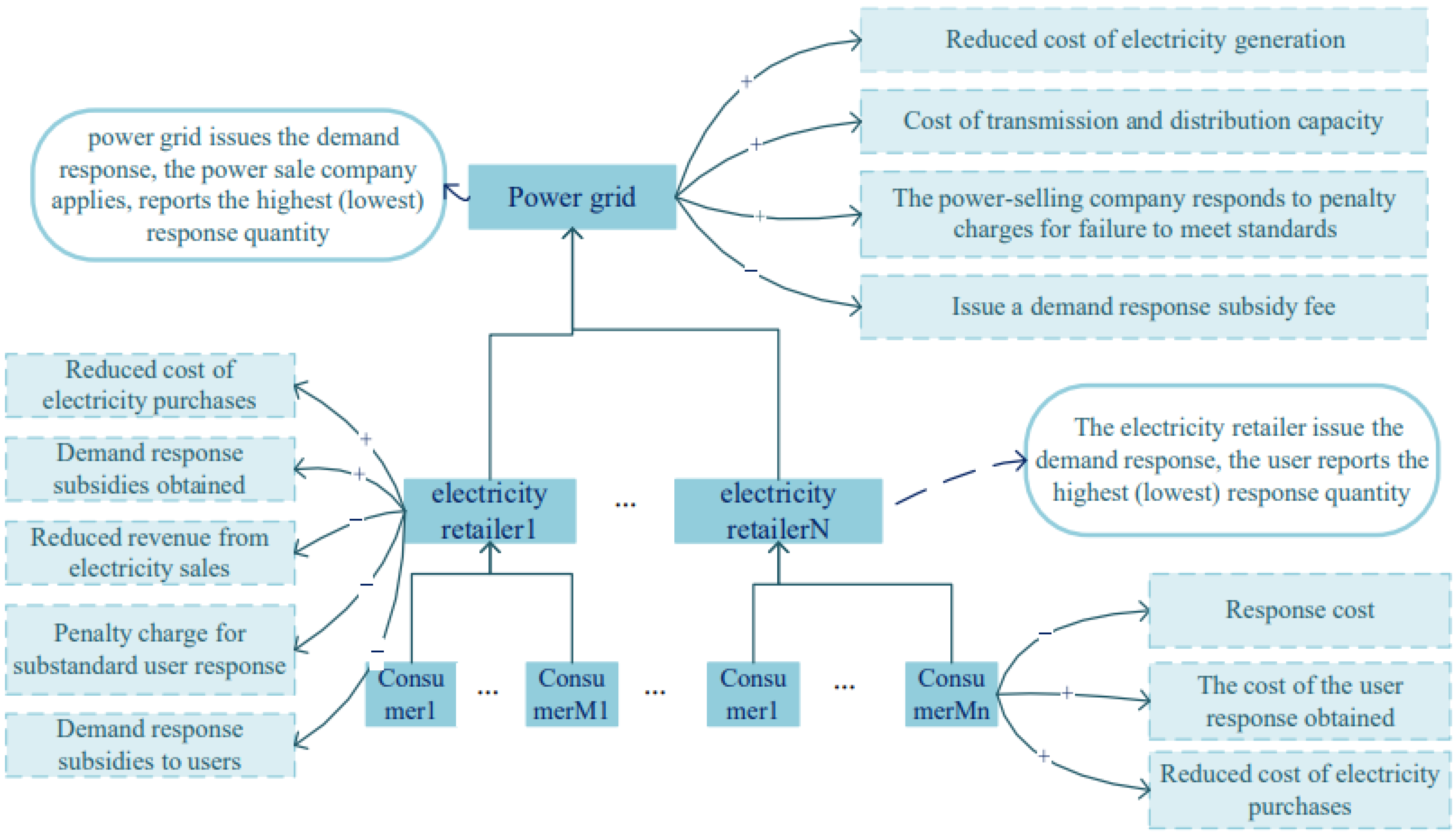
This paper considered the competition relationship between the three parties of “power grid–electricity retailer–user” and constructs a two-layer master–slave game model, as depicted in Figure 1. The higher-level demand response model involves the grid, which acts as a leader in the game. The grid publishes demand responses and takes into account constraints based on market electricity prices and electricity sales. The subsidy unit price of each electricity sales company is set with the aim of maximizing the grid’s own income. Each electricity retailer in the lower-level model acts as a follower. After receiving the demand response information of the grid, they optimize their internal response volume and subsidy price to the user with the aim of maximizing their own revenue. The grid then adjusts the subsidy price according to the response strategy of the electricity retailer. This process creates a leader–follower sequential game and constitutes a Stackelberg game relationship [22], as well as a non-cooperative game relationship between each electricity seller.

In the lower-level model, the electricity sales company plays the role of a leader, publishes demand responses, combines its own power purchase constraints, and sets the subsidy unit price of each user with the goal of maximizing its personal income. Each user also acts as a follower. After receiving the demand response information from the electricity retailer, they optimize the response volume and power purchase period in order to maximize their own income. The electricity retailer then adjusts the subsidy price again based on the user’s response strategy. This creates a leader–follower sequential game, constituting a Stackelberg game relationship. Each user also constitutes a non-cooperative game relationship in this model.

3.2. Game Model Solving

The game flow is as follows: The game model proposed earlier transforms the demand-side electricity purchasing decision problem into a multi-objective optimization problem, enabling more comprehensive and scientific purchasing decisions. The MOMVO algorithm [23] is a global search optimization algorithm with strong convergence speed, fast convergence rate, and good robustness, and it has been widely applied in many fields. In this paper, the game model was combined with the MOMVO algorithm by converting the objective functions and constraints in the master–slave game model into multiple fitness functions, and using the MOMVO algorithm to solve it. This method not only improves the efficiency of solving game models but also provides a new method for addressing optimization problems with multiple objectives.

The MOMVO algorithm utilizes the multiverse theory [24], which regards each optimal solution as a universe, to find all optimal solutions by simulating the interaction and variation of universes. The algorithm includes steps such as population initialization, individual evaluation, individual selection, individual evolution, and determining stopping conditions, and ultimately outputs all the found optimal solutions. This algorithm boasts several benefits, including potent global search capability, swift convergence speed and exceptional robustness, and has found extensive application across various domains.

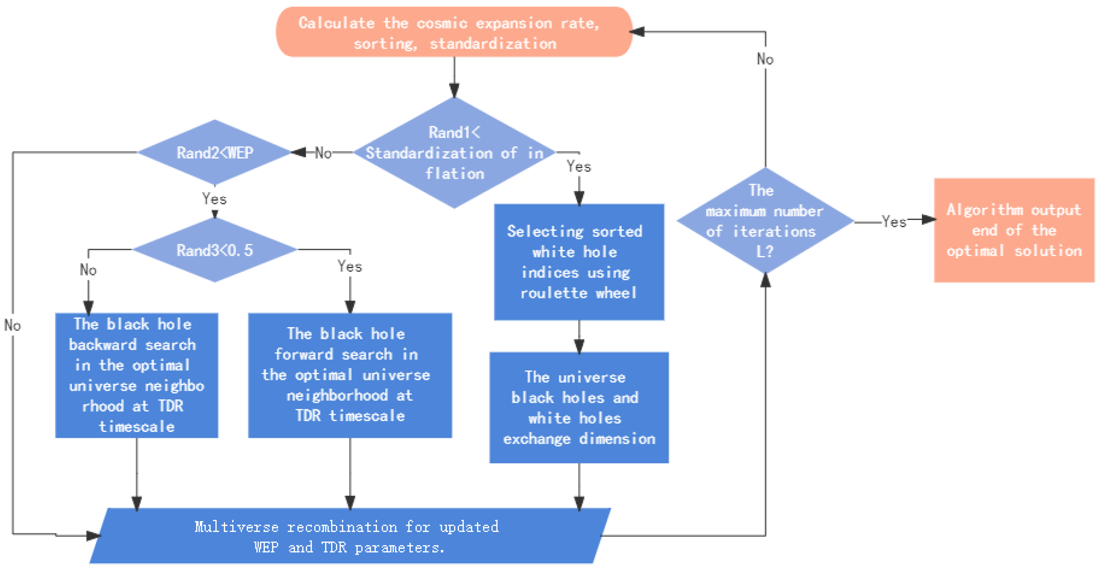
The MVO algorithm is based on the multiverse theory’s three main concepts: white hole, black hole, and wormhole. It establishes a mathematical model for optimization with candidate solutions defined as universes and their fitness measured by expansion rates. Each iteration uses black holes as candidate solutions, selecting better universes as white holes via roulette wheel selection. Black and white holes exchange their contents while some black holes can use wormholes to search for the best universes. The algorithm’s internal loop structure’s logical flow is illustrated in Figure 2.

In Figure 2, black holes update dimensions using two mechanisms.

(1) Based on sorted normalized expansion rates, white hole indices are selected using the roulette wheel selection principle and black holes exchange dimensional information with the selected white hole.

(2) When $Rand2<WEP$, black holes travel through wormholes and update their dimensions using $TDR$ parameters in the optimal universe neighborhood. The iteration Formula (22) is used, with j representing the specific dimension of the optimized problem.

$$X_j^i=\left\{\begin{array}{ccc}\hfill Best{X}_j-TDR(u{b}_j-l{b}_j)·rand+l{b}_j,& \hfill & \hfill Rand3\ge 0.5\\ \hfill Best{X}_j+TDR(u{b}_j-l{b}_j)·rand+l{b}_j,& \hfill & \hfill Rand3<0.5\end{array}\right.$$

(22)

$$TDR=1-{(\frac{1}{Len})}^{\frac{1}{6}}$$

(23)

$$WEP=WE{P}_{min}+\frac{1en}{Len}·(WE{P}_{max}-WE{P}_{min}).$$

(24)

In Formulas (22)–(24), $len$ and $Len$ represent the current and maximum iterations, $ub$ and $lb$ represent the boundaries of the problem, $BestX$ represents the position of the optimal universe, and $WEP$ and $TDR$ are important parameters of the Multiverse Optimization Algorithm for the probability of wormhole existence and the travel distance rate. Formula (23) indicates that the $TDR$ parameter of the Multiverse Optimization Algorithm is a concave decreasing function during the iteration, decreasing rapidly at first and gradually slowing down, while the WEP parameter increases linearly.

MOMVO is the multi-objective version of MVO, designed to store the best non-dominant solutions. To select the best solutions from the archive, a tunnel is established between solutions using the leader selection mechanism. In this approach, the crowding distance between each solution in the archive is initially selected, and the number of solutions in its neighborhood is used as a measure of coverage or diversity. MOMVO uses roulette wheel selection to improve the distribution of solutions across all objectives, favoring solutions with fewer individuals in the archive. The following equation is used to achieve this improvement.

$$P_r=h/N_m.$$

(25)

Using a constant parameter h greater than 1 and kept constant, the equation favors solutions near the i-th solution while reducing the fitness of hypercubes with more particles as a form of fitness sharing. This equation provides high probability solutions for regions with fewer solutions, improving other areas and attracting solutions to these regions with fewer individuals in the archive. It ultimately increases the coverage of the obtained Pareto optimal front.

Archives can only accommodate a limited number of non-dominated solutions and can become full during the optimization process. Therefore, a mechanism is needed to remove unnecessary solutions from the archive. An unnecessary solution is one that is surrounded by many solutions and thus requires cleanup to save space. The inverse Equation (26) is used to discard unwanted solutions from the archive and provide high probability for the MOMVO algorithm.

$$P_r^{\prime }=N_m/h.$$

(26)

To quantify convergence, this paper selected the generational distance (GD) [25] and inverted generational distance (IGD) [26] proposed by Veldhuizen in 1998. These performance metrics serve to quantify the distribution of Pareto optimal solutions obtained. The corresponding mathematical equations for these performance measures are as follows:

$$GD=\frac{\sqrt{{\sum }_{i_1=1}^{no}{s_i}_1^2}}{no}$$

(27)

$$IGD=\frac{\sqrt{{\sum }_{i_2=1}^{nt}{\left({s_i^{\prime }}_2\right)}^2}}{nt},$$

(28)

where $no,nt$ indicate the count of Pareto optimal solutions, and ${s_i}_1,{s_i}_2^{\prime }$ represent the Pareto optimal solution, and reference concentration is the most close to the true Pareto optimal solutions of m Euclidean distance. Please note that the Euclidean distances are calculated respectively in their target space.

In order to assist decision makers in selecting the optimal solution from the Pareto frontier, this paper modified the weights of individual indicators using a comprehensive evaluation index method and integrated them into a single objective function. The considered indicators included grid revenue, electricity retailer revenue, user revenue, peak load (valley filling) reduction, user electricity consumption comfort, and participation response satisfaction. The changes in indicator weights are related to the fairness of demand response and the optimal strategy chosen by the decision maker.

The electricity consumption comfort level u of users represents the sum of the standard deviations of the response volume in which all users are involved in the demand response, as in Equation (29). User satisfaction v represents the sum of the standard deviations of the unit price of subsidies obtained by all users participating in demand response, as shown in Equation (30), where M is a collection of all users, and $i=1,2,...,M$.

$$u=\sum _{t=1}^T\sum _{i\in M}\sqrt{\left({\tilde{q}}_i^t\right)-{\overline{\tilde{q}}}_i^t{)}^2},t=1,2,\dots ,T,i\in M$$

(29)

$$v=\sum _{t=1}^T\sum _{i\in M}\sqrt{{({\tilde{r}}_i^t-{\overline{\tilde{r}}}_i^t)}^2},t=1,2,\dots ,T,i\in M.$$

(30)

In the model, the weight coefficient matrix of each index is formulated as $\mathbf{l}=(l_{U_G},l_{U_S},l_{U_E},l_Q,l_u,l_v)$, where $l_{U_G},l_{U_S},l_{U_E},l_Q,l_u,l_v$ represent the weights of grid, electricity retailer, user revenue, peak load (valley filling) reduction, user electricity consumption comfort, and participation response satisfaction, respectively. The process of determining the indicator weights in this paper involved employing the CRITIC method, as expounded in [27], which is an objective weighting method that is superior to entropy weighting and standard deviation weighting methods. The CRITIC method takes into account the conflict and contrast intensity among indicators, and can simultaneously consider the size and correlation of indicator variability, using the inherent properties of the data for scientific evaluation.

4. Example Analysis

The reform of China’s electricity spot market is in its early stages, with limited marketization and trading volume, making it difficult to obtain real-time electricity price data due to the need for mature market mechanisms and trading platforms for accurate price determination and real-time data acquisition. Therefore, this paper used real-time electricity price data from established electricity markets, such as PJM, which can be more practical and reliable. This paper selected data from one day in the PJM market to verify and analyze the model, which has a total of 24 time periods. In the power grid’s demand response implementation phase, there could be multiple electricity retailers who are interested in taking part in the demand response program. This paper considered one power grid company, two electricity retailers, and three users participating in the demand response released by the electricity retailers. It was assumed that the total maximum response capacity of the users can meet the power grid’s maximum response demand.

4.1. Parameter Settings

The user’s time-of-use pricing schedule was set in intervals as shown in

Table 1. Time-of-use price contract time segment of users.

Type	Period of Time
Valley period	1, 2, 3, 4, 5, 6, 23, 24
Normal period	7, 8, 13, 14, 15, 16, 17, 18
Peak period	9, 10, 11, 12, 19, 20, 21, 22

, while the utility company’s time-of-use pricing is presented in

Table 2. Time-of-use price of electricity retailers.

	Valley Period	Normal Period	Peak Period
electricity retailers A ($/MWh)	28.26	34.42	38.33
electricity retailers B ($/MWh)	26.21	33.65	39.21

. The differentiated elasticity coefficient for users was also set simultaneously, as shown in

Table 3. Customers differentiation elasticity.

Type of Load	Coefficient of Self-Elasticity	Cross Elastic Coefficient
		Peak-Normal	Peak-Valley	Normal-Valley
user1	−0.05	0.02	0.04	0.02
user2	−0.12	0.02	0.03	0.11
user3	−0.38	0.03	0.23	0.03
user4	−0.56	0.02	0.04	0.02
user5	−0.14	0.15	0.03	0.18
user6	−0.23	0.03	0.08	0.06

, while the response cost coefficient for different users is presented in

Table 4. Response cost coefficient of different consumers (unit: $(MW·h)${}^{-1}$).

User	Response Cost Factor $\mathit{\beta }$	Response Cost Factor $\mathit{\gamma }$
user1	0.2	60
user2	0.2	62
user3	0.2	58
user4	0.2	58
user5	0.2	60
user6	0.2	56

.

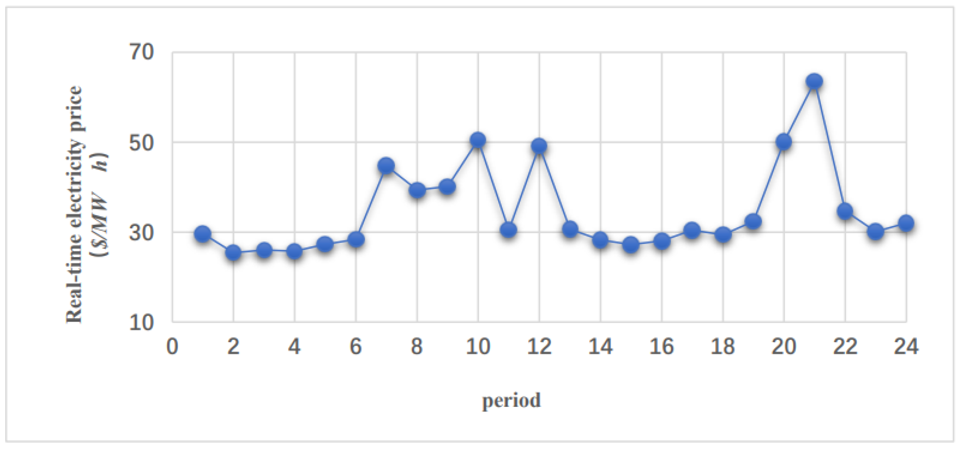
The cost-per-unit of avoiding transmission and distribution capacity in the power grid was set at 2 $/MW, while the transmission and distribution loss coefficient was $\alpha =0.04$, and the cost coefficient for power generation was $a=0.06$, $b=20$, and $c=5$. The originally planned power output capacity for the day was $Q=6000$ MW·h, and Figure 3 illustrates the live electricity rate prediction value. The grid plans to release a peak-shaving demand response project during the high-load peak period, which lasts for two hours (19:00–21:00).

4.2. Scene Settings

This paper proposed a master–slave game model and used Python for simulation programming to obtain the equilibrium solution of the game between the power grid, retail electricity companies, and users. Four scenarios were set up for comparative analysis to verify the effectiveness of the optimization strategy, with different algorithms used to solve the game model’s optimal solution while considering the impact of price elasticity on user demand response.

• Scenario 1 did not consider price elasticity on user demand response and used the MOMOV algorithm to solve the game model’s optimal solution.
• Scenario 2 considered price elasticity and used the MOMOV algorithm.
• Scenario 3 considered price elasticity and used the MOPSO algorithm to solve the game model’s optimal solution.
• Scenario 4 considered price elasticity and used the NSGA-II algorithm to solve the game model’s optimal solution.

4.3. Comparative Analysis

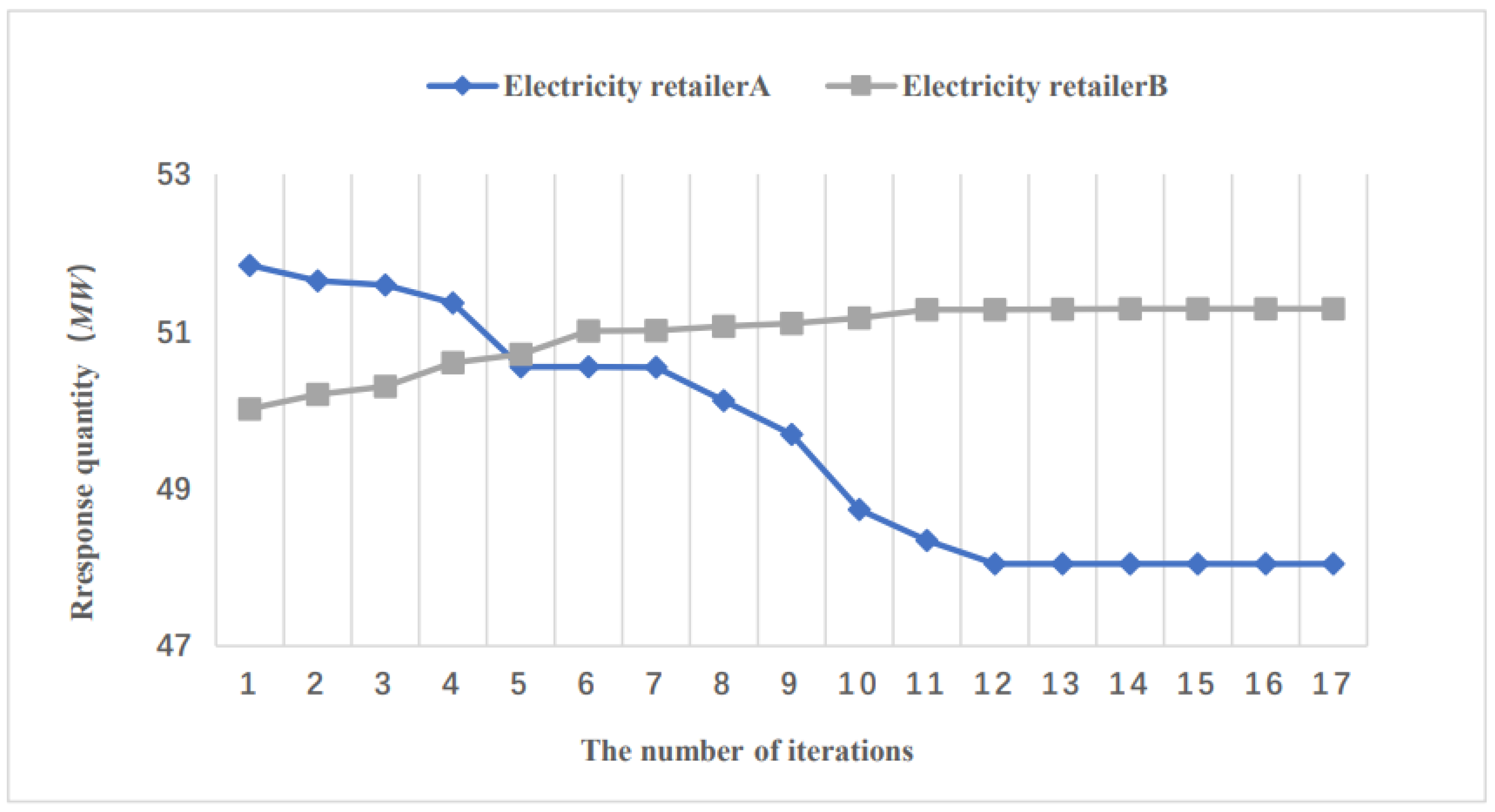
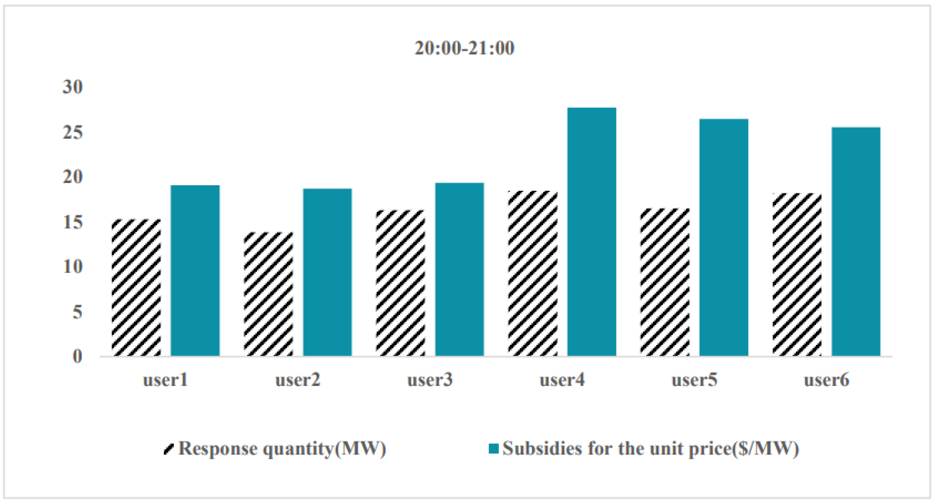
When using the MOMOV algorithm for solving, $Len$ was set to 100, while $WEP$ linearly increased from 0.2 to 1 and $TDR$ decreased concavely from 0.6 to 0. According to Scenario 1, the model converged in the 16th iteration. The optimal response of the retail electricity companies showed a convergence trend as the iteration increased, as shown in Figure 4.

Table 5. The optimal response quantity and subsidy unit price of electricity retailers.

Electricity Retailers	Period	Response Amount ($/MW)	Subsidy Unit Price ($/MW·h)
electricity retailers A	19:00–20:00	48.044	24.64
	20:00–21:00	49.068	25.07
electricity retailers B	19:00–20:00	51.417	27.09
	20:00–21:00	51.057	26.35

shows the optimal response of the retail electricity companies and their corresponding subsidy price. Figure 5 shows the optimal response and subsidy price of users during the 20:00–21:00 period. It can be seen that user 4 has the highest response and subsidy price at 27.16 MW and 18.53 USD/MW, respectively, while user 2 has the lowest response and subsidy price at 18.85 MW and 13.37 USD/MW, respectively. When the user response is high, a corresponding high subsidy price can be obtained to stimulate users to increase their response.

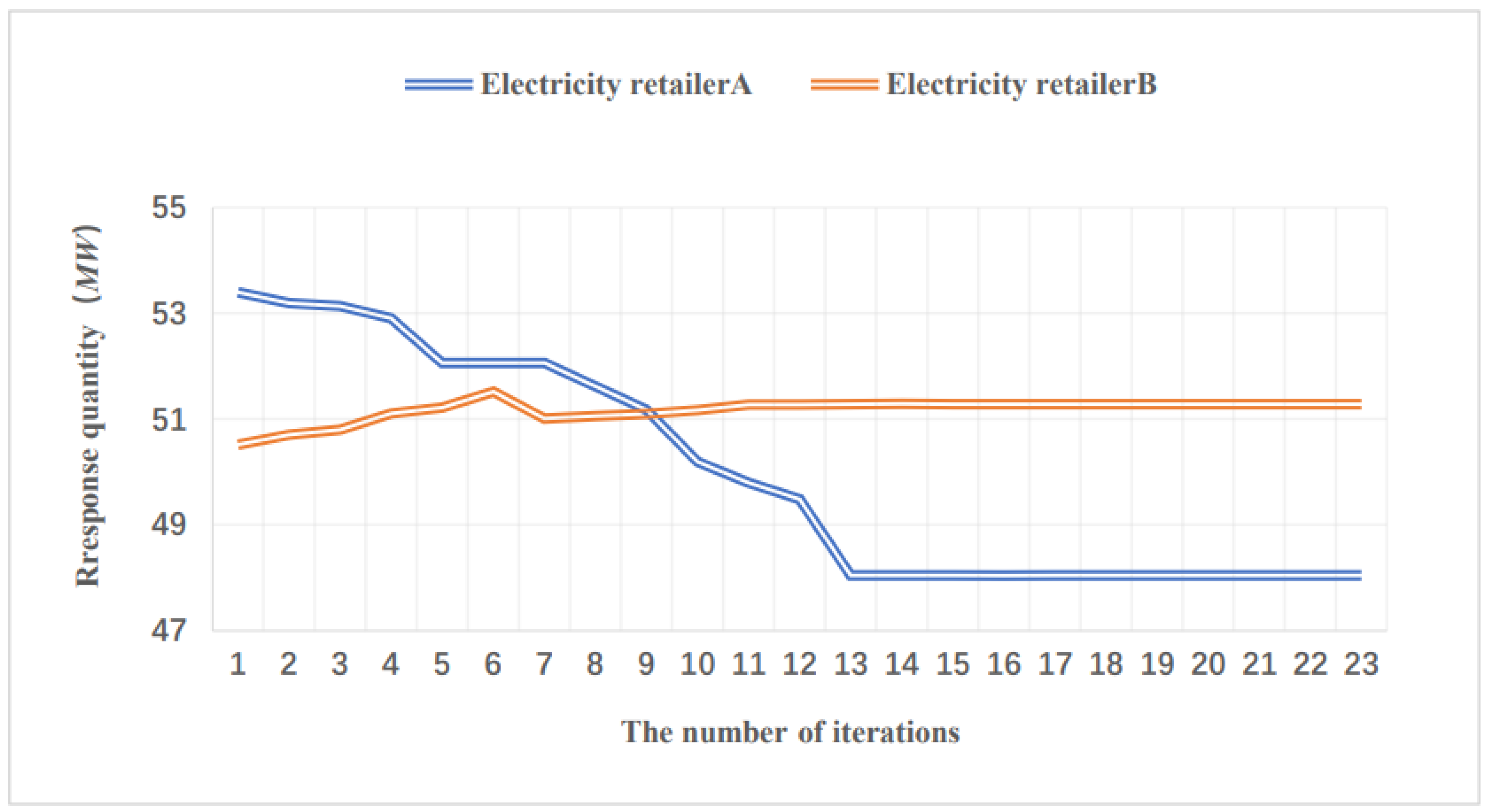
In Scenario 2, considering the elasticity of users, the optimal response of the power company converged in the 18th iteration as shown in Figure 6. The optimal response of Retail Electricity Company A was 48.04 MW, and the optimal response of Retail Electricity Company B was 50.87 MW. At this time, the power grid’s revenue was USD 3315.33 and the revenues of the two retail electricity companies were USD 2324.60 and USD 2420.37, respectively.

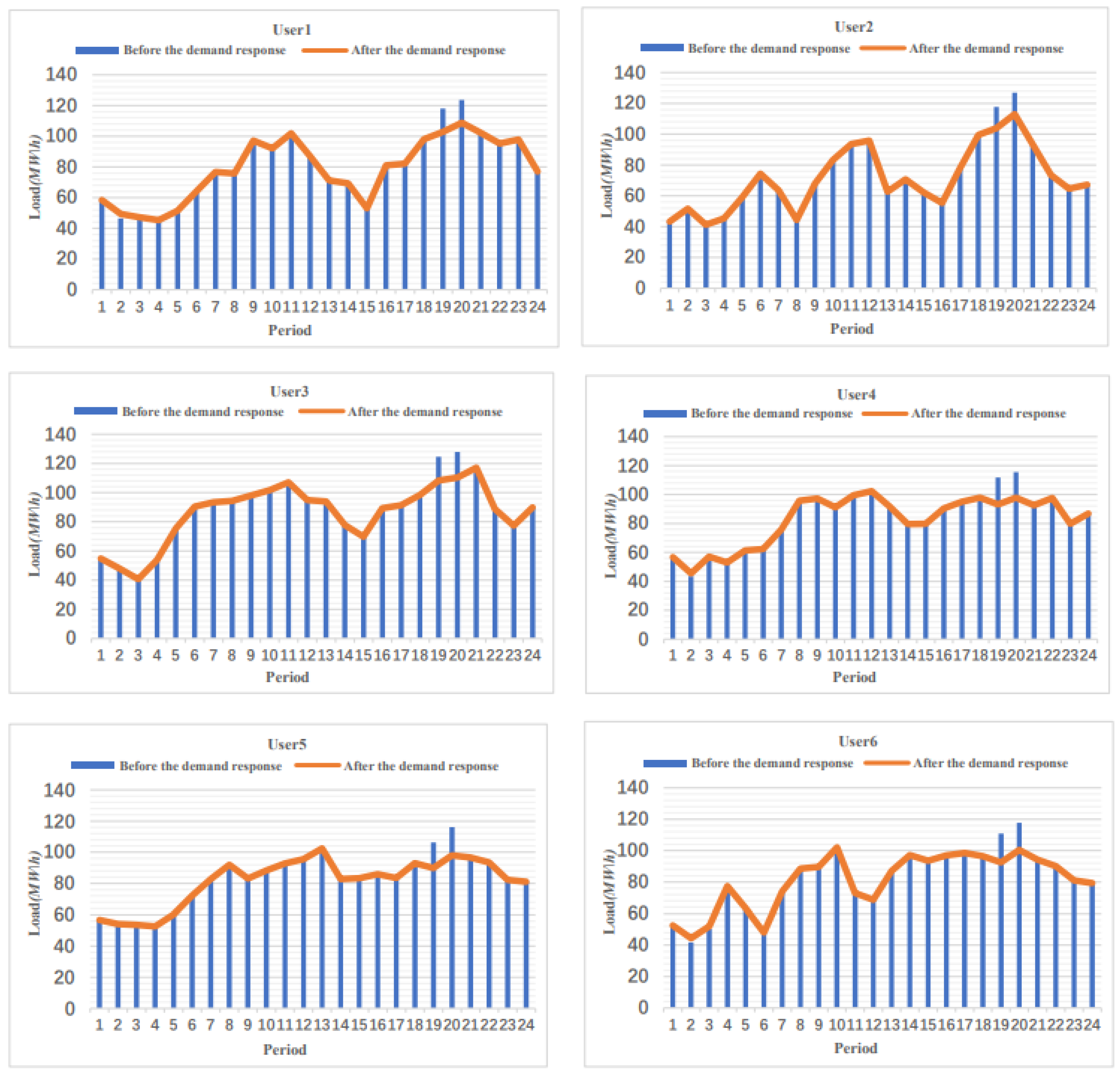
Figure 7 shows the comparison of load before and after demand response by electricity users. It is evident from the figure that there is a significant decrease in the load during peak hours and an increase in electricity consumption during off-peak hours. Among all users, user 6 had the highest decrease in load during the 19:00–20:00 period, reaching 15.97%, while user 1 had the highest increase in electricity consumption, reaching 6.09%. By participating in demand response, users reduce their electricity costs and have a more stable load curve, reducing the losses caused by the extreme imbalance of power generation in the power grid while considering the price elasticity of demand response. User 4 had the highest price elasticity of demand response, resulting in the highest electricity consumption transfer, which was 1.13%. Through participation in demand response, users can reduce their power purchase costs while also making their load curve smoother, thereby reducing the losses caused by extreme power generation imbalance in the power grid.

In both Scenario 1 and Scenario 2, the MOMOV algorithm was used, but Scenario 2 took into account the elasticity coefficients of the users. The results of the two scenarios are shown in

Table 6. Demand response in different scenarios.

Scenario	Response Cost Factor Grid Revenue ($)	Total Response (MW)	Load Transfer Amount (MW)
Scenario 1	3267.31	193.06	0
Scenario 2	3345.33	198.64	13.36

. The table shows that, in Scenario 2, the total user response increased by 2.89% and the power grid’s benefits increased by 2.39%. It is evident that, in the process of maximizing its own benefits, the power grid company may sacrifice user benefits, which reduces the enthusiasm of users to participate in response. However, when considering the elasticity coefficients of users, the transfer of load reduces the user’s response cost and increases their response enthusiasm, while optimizing the regulation of the power grid.

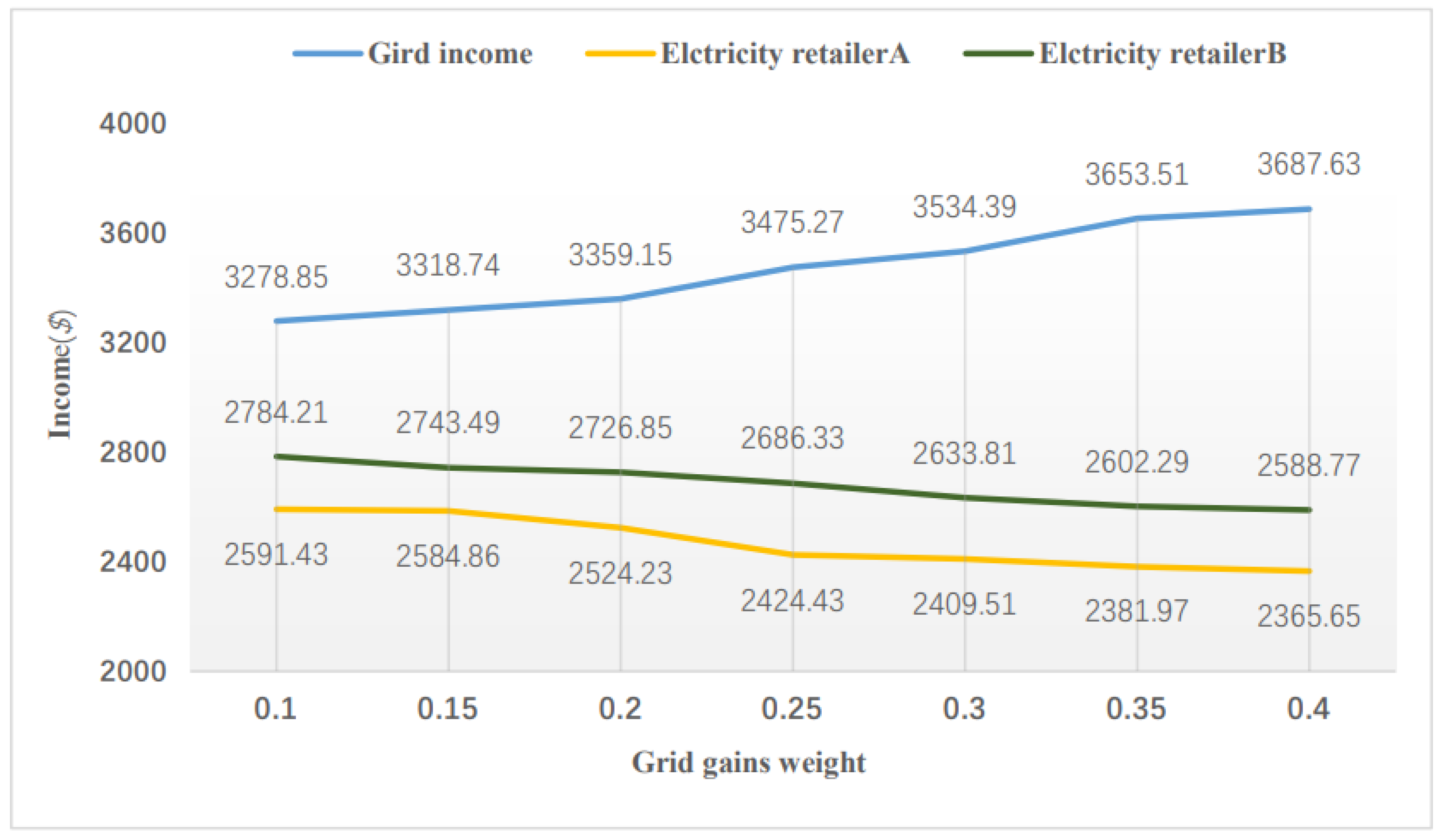
In Scenario 2, when adjusting the profit weight $l_{U_G}$ of the power grid while ensuring that other weight proportions remain unchanged, the changes in the profits of the power grid and electricity retailers are shown in Figure 8. When the profit weight $l_{U_G}$ of the power grid increased from 0.1 to 0.4 under optimal decision-making, the profit of the power grid increased by 12.46%, while the profits of electricity retailer A and B decreased by 8.71% and 7.02%, respectively. In the game, as the profit weight of the power grid increased and the response subsidies received by electricity retailers decreased, their profits decreased.

With all other parameter values being equal, the results of solving Scenarios 2, 3, and 4 were compared. In other words, the effectiveness of the MOMOV, MOPSO, and NSGA-II algorithms for solving the game model was compared when taking into account the elasticity coefficients of users. The model was solved using each algorithm, independently run 20 times. The average and standard deviation of the IGD indicator were calculated, as shown in

Table 7. Results of the multi-objective algorithms (using GD, IGD) on the model.

MOPSO		NSGA-II		MOMOV
GD	IGD	GD	IGD	GD	IGD
4.18 $\times {10}^{-3}$	1.32 $\times {10}^{-2}$	3.27 $\times {10}^{-3}$	2.12 $\times {10}^{-2}$	1.60 $\times {10}^{-4}$	4.10 $\times {10}^{-3}$

. It can be seen that the MOMOV algorithm performed the best in solving the model, with the smallest IGD indicator and standard deviation, indicating that this algorithm is more stable and effective than the other two algorithms. Therefore, the experimental findings serve as a testament to the efficacy of the MOMOV algorithm in addressing the decision variable contribution target analysis method for this particular model.

5. Conclusions

This paper addressed the demand response of the grid and proposed a game-theoretic model among grid, electricity retailers, and multiple users employing the master–slave game approach. Through the analysis and solution of the model, game equilibrium was achieved, and the corresponding strategy for power grid companies to set demand response subsidy prices was obtained. The simulation results of the example showed that the demand response game model constructed can achieve established goals, and the use of MOMOV for solving the model was superior to other optimization algorithms, which to some extent verified the rationality of the article. The subsidy price formulation strategy proposed in this paper not only considers user participation in demand response and reducing direct response subsidies, but also considers that users adjust their own electricity consumption under the influence of the price elasticity coefficient, and shift peak electricity consumption to valley hours. While users gain benefits, it has contributed positively to the process of reducing peak demand and filling low demand periods for the power system and effectively utilizing funds to improve the overall revenue of the grid in a competitive market environment. This has positive implications, while also providing a new train of thought for future demand response subsidized prices.

References

1. Zhang, G.; Xue, S.; Fan, M.; Zhang, H. Design of market-oriented trading mechanism for demand response to China’s electricity market. Electr. Power Constr. 2021, 42, 132–140. [Google Scholar]
2. Song, Y.; Bao, M.; Ding, Y.; Shao, C.; Shang, N. Review of Key Points and Related Suggestions of China’s Electricity Spot Market Construction under New Power Reform. Proc. CSEE 2020, 40, 3172–3187. [Google Scholar]
3. He, Q.; Ai, Q. Bidding Strategy of Electricity Market with Demand Response virtual power plant in the environment of power sales side liberalization. Electr. Power Constr. 2019, 3, 2–6. [Google Scholar]
4. Wang, T.; Xu, K.; Zhu, Y. Source-grid-load multilayer game economic dispatching strategy of active distribution network. Power Syst. Prot. Control 2018, 46, 10–19. [Google Scholar]
5. Wang, H.; Xu, H.; Zhao, W. Optimization of multi-agent trading decisions in electricity market under uncertain demand and quota system. Power Grid Clean Energy 2021, 37, 34–44. [Google Scholar]
6. Sun, L.; Wang, Y.; Ding, J.; Ding, M.; Wang, P. Robust Planning Strategy for Generation and Transmission Considering Incentive Demand-Side Response. Electr. Power Constr. 2022, 43, 63–72. [Google Scholar]
7. Sun, Q.; Wang, X.; Wang, Y.; Zhang, Y.; Liu, Z.; He, J. Integrated energy market transaction optimization decision based on multi-agent Nash-Q reinforcement learning. Power Syst. Autom. 2021, 45, 10. [Google Scholar]
8. Cai, G.; Jing, Y.; Huang, N.; Yang, D.; Pan, X.; Shang, W. Optimal Scheduling of Charge and Discharge of Large-scale Electric Vehicles Based on Multi-agent Two-Layer Game under Power Demand Response Mechanism. Proc. CSEE 2023, 43, 14. [Google Scholar]
9. Lu, Q.; Zhang, Y. Demand response strategy of game between power supply and power consumption under multi-type user mode. Int. J. Electr. Power Energy Syst. 2022, 134, 107348. [Google Scholar] [CrossRef]
10. Dai, Y.; Sun, X.; Li, L.; Gao, H. Real-time Demand Response Mechanism of Smart Grid Residential Power Based on Multi-layer Game. Oper. Res. Manag. 2021, 30, 11–17. [Google Scholar]
11. Dai, Y.; Sun, X.; Qi, Y.; Leng, M. A real-time, personalized consumption-based pricing scheme for the consumptions of traditional and renewable energies. Renew. Energy 2021, 180, 452–466. [Google Scholar] [CrossRef]
12. Apostolopoulos, P.A.; Tsiropoulou, E.E.; Papavassiliou, S. Demand response manage-ment in smart grid networks: A two-stage game-theoretic learning-based approach. Mob. Netw. Appl. 2021, 26, 548–561. [Google Scholar] [CrossRef]
13. Wu, C.; Gao, B.; Tang, Y.; Wang, Q. Master–slave Game Based Bilateral Contract Transaction Model for Generation Companies and Large Consumers. Autom. Electr. Power Syst. 2016, 40, 56–62. [Google Scholar]
14. Cheng, L.; Yin, L. Behav-ioral decision-making in power demand-side response management: A multi-population evolutionary game dynamics perspective. Int. J. Electr. Power Energy Syst. 2021, 129, 106743. [Google Scholar] [CrossRef]
15. Lu, Q.; Lv, S.; Leng, Y. A Nash-Stackelberg game approach in regional energy market considering users’ integrated demand response. Energy 2019, 175, 456–470. [Google Scholar] [CrossRef]
16. Motalleb, M.; Siano, P.; Ghorbani, R. Networked Stackelberg competition in a demand response market. Appl. Energy 2019, 239, 680–691. [Google Scholar] [CrossRef]
17. Dai, Y.; Gao, H.; Gao, Y.; Yuan, G. Real-time pricing mechanism in smart grid with forecasting update of power demand. Autom. Electr. Power Syst. 2018, 42, 58–63. [Google Scholar]
18. Lin, K.; Wu, J.; Liu, D.; Li, D. Energy management optimization of micro energy grid based on hierarchical Stackelberg game theory. Syst. Technol. 2019, 43, 973–983. [Google Scholar]
19. Mirjalili, S.; Jangir, P.; Mirjalili, S.Z.; Saremi, S.; Trivedi, I.N. Optimization of problems with multiple objectives using the multi-verse optimization algorithm. Knowl.-Based Syst. 2017, 134, 50–71. [Google Scholar] [CrossRef]
20. Lin, G.; Lu, S.; Guo, K.; Gao, Z.; Feng, X. Pricing Mech-anism of Demand Response Subsidy for Power Grid Companies Based on master–slave Game. Power Syst. Autom. 2020, 44, 59–67. [Google Scholar]
21. Xue, W.; Zhao, X.; Li, Y.; Mu, Y.; Tan, H.; Jia, Y.; Wang, X.; Zhao, H.; Zhao, Y. Research on the Optimal Design of Seasonal Time-of-Use Tariff Based on the Price Elasticity of Electricity Demand. Energies 2023, 16, 1625. [Google Scholar] [CrossRef]
22. Zhang, H.; Zhang, S.; Cheng, H.; Zhang, X.; Gu, Q. A Review of the Application of Stackelber Game in Electricity Market. Trans. China Electrotech. Soc. 2022, 37, 3250–3262. [Google Scholar]
23. Kumari, K.; Kumar, N.C.; Ranjan, N.M. Electric vehicles management enabling G2V and V2G in smart distribution system for maximizing profits using MOMVO. Int. Trans. Electr. Energy Syst. 2019, 29, e12013. [Google Scholar]
24. Haseeb, A.; Waleed, U.; Ashraf, M.M.; Siddiq, F.; Rafiq, M.; Shafique, M. Hybrid Weighted Least Square Multi-Verse Optimizer (WLS–MVO) Framework for Real-Time Estimation of Harmonics in Non-Linear Loads. Energies 2023, 16, 609. [Google Scholar] [CrossRef]
25. David, A.; VanVeldhuizen Gary, B. Lamont. Evolutionary Computation. In Evolutionary Computation; Massachusetts Institute of Technology Press: Cambridge, MA, USA, 1999. [Google Scholar]
26. Sierra, M.R.; Coello, C.A.C. Improving PSO-Based Multi-Objective Optimization Using Crowding, Mutation and—Dominance. In Proceedings of the Evolutionary Multi-Criterion Optimization, Guanajuato, Mexico, 9–11 March 2005; pp. 505–519. [Google Scholar]
27. Zhao, S.; Tang, S. Comprehe-nsive Evaluation of Transmission Network Planning Scheme Based on Improved Analytic Hierarchy Method, CRITIC Method and Approximation Ideal Solution Ranking Method. Electr. Power Autom. Equip. 2019, 39, 143–148+162. [Google Scholar]
Figure 1. Tripartite demand response decision model of “power grid, electricity retailers and consumers”.
Energies 16 04009 g001
Figure 2. The algorithm’s internal loop structure’s logical flow.
Energies 16 04009 g002
Figure 3. Real-time electricity price forecast value of power grid.
Energies 16 04009 g003
Figure 4. Convergence process of the optimal response quantity of the electricity retailers in Scenario 1.
Energies 16 04009 g004
Figure 5. The optimal response quantity and subsidy unit price of users during 20:00–21:00.
Energies 16 04009 g005
Figure 6. Convergence process of the optimal response quantity of the electricity retailers in Scenario 2.
Energies 16 04009 g006
Figure 7. Load change before and after users participate in demand response.
Energies 16 04009 g007
Figure 8. Response income with the participation of power grid and electricity retailers with the change of income weight of power grid.
Energies 16 04009 g008