Ellipsoidal Design of Robust Stabilization of Power Systems Exposed to a Cycle of Lightning Surges Modeled by Continuous-Time Markov Jumps

Abstract

Power system stability is greatly affected by two types of stochastic or random disturbances: (1) topological and (2) parametric. The topological stochastic disturbances due to line faults caused by a series of lightning strikes (associated with circuit breaker, C.B., opening, and auto-reclosing) are modeled in this paper as continuous-time Markov jumps. Additionally, the stochastic parameter changes e.g., the line reactance, are influenced by the phase separation, which in turn depends on the stochastic wind speed. This is modeled as a stochastic disturbance. In this manuscript, the impact of the above stochastic disturbance on power system small-disturbance stability is studied based on stochastic differential equations (SDEs). The mean-square stabilization of such a system is conducted through a novel excitation control. The invariant ellipsoid and linear matrix inequality (LMI) optimization are used to construct the control system. The numerical simulations are presented on a multi-machine test system.

1. Introduction

1.1. Brief Review

Power system stability is the most important issue in power system operation. The stability problem has become ever prominent, greatly endangering the safe and stable operation of a power system, even causing blackouts, which result in immeasurable losses to society and the economy. Power systems are vulnerable to stochastic fluctuations, which can be divided into three categories:

(1)

topological randomness (e.g., line faults);

(2)

parametric randomness (e.g., in the state matrix coefficients, which is caused by the parameters changes in the system equipment);

(3)

exogenous stochastic disturbances, such as variations in wind turbine mechanical power inputs.

Although randomness always exists in power systems, traditional stability studies remain almost deterministic. Considerable results exist on deterministic power system dynamic stability [1,2]. Conventional PSS may fail when the operating point changes [1]. Different designs of PSS which are robust against load changes exist. In [3], the authors use Kharitonov’s theorem to robustify the conventional PSS. In [4,5], the authors provide reliable PSS/governor control; even if either controller fails, the system stays stable. The practical control signal limits of PSS are presented in [6]. Wavelet-based PSS design is shown in [7]. The authors of [8] present the fuzzy switching of regional PSS pole placers without violating the control input limits. Robust decentralized PID-PSS design by iterative LMI is given in [9]. The uncertainty in the PSS’s parameters is shown in [10]. Graphical selection of the robust PID-PSS is given in [11].

Unlike deterministic stability, which is described by ordinary differential equations, stochastic differential or difference equations describe the dynamics of a system under random variations. In the field of stochastic stability for power systems, little research has been performed. The probabilistic eigenvalue analysis is used in [12,13,14] to construct a power system stabilizer that improves small-disturbance stability. Ref. [15] shows how to represent power system stabilization during sudden load changes using a Markov chain. Ref. [16] deals with cascading failure. The authors of [17] investigate the stabilization of a system after a succession of lightning strikes. However, as long as they are created on ordinary differential equations, these methods are not ideal for investigating the influence of stochastic disturbances.

The field of power system stochastic dynamics is relatively new. As shown in [18], it is approached as a stochastic differential equation (SDE). Ref. [19] gives a clear overview of SDEs. Wind power generation with stochastic wind speed variation is solved by SDEs in [20,21,22].

This manuscript introduces Itô’s stochastic calculus as the main tool for the stochastic stability problem. The stochastic power systems parameter uncertainties are considered as an external disturbance modeled as a Wiener (or Brownian) process. A continuous-time Markov process [23,24] is used to describe the power system under a string of lightning strikes, and the system state equation is derived using SDE. The system state equation is derived to model disturbance stability. Then an excitation control to achieve small stochastic mean-square stability and minimize the impact of the external disturbance is demonstrated [25]. The new proposed control design is derived based on the invariant (attractive) ellipsoid [26,27] and linear matrix inequalities (LMIs) optimization. Numerical simulations of the system response are carried out using the Euler–Milstein method.

1.2. The Most Important Contributions

The most important contributions in this work are:

• SDE modeling of a multi-machine system under a succession of lightning surges by continuous-time Markov jumps (representing the topology uncertainty) + external disturbance (representing the stochastic parameter uncertainty).
• A new sufficient condition for stochastic stability is derived where the external disturbance is rejected by minimizing the volume of the invariant (attractive) ellipsoid.
• A simple design of the excitation control is presented.
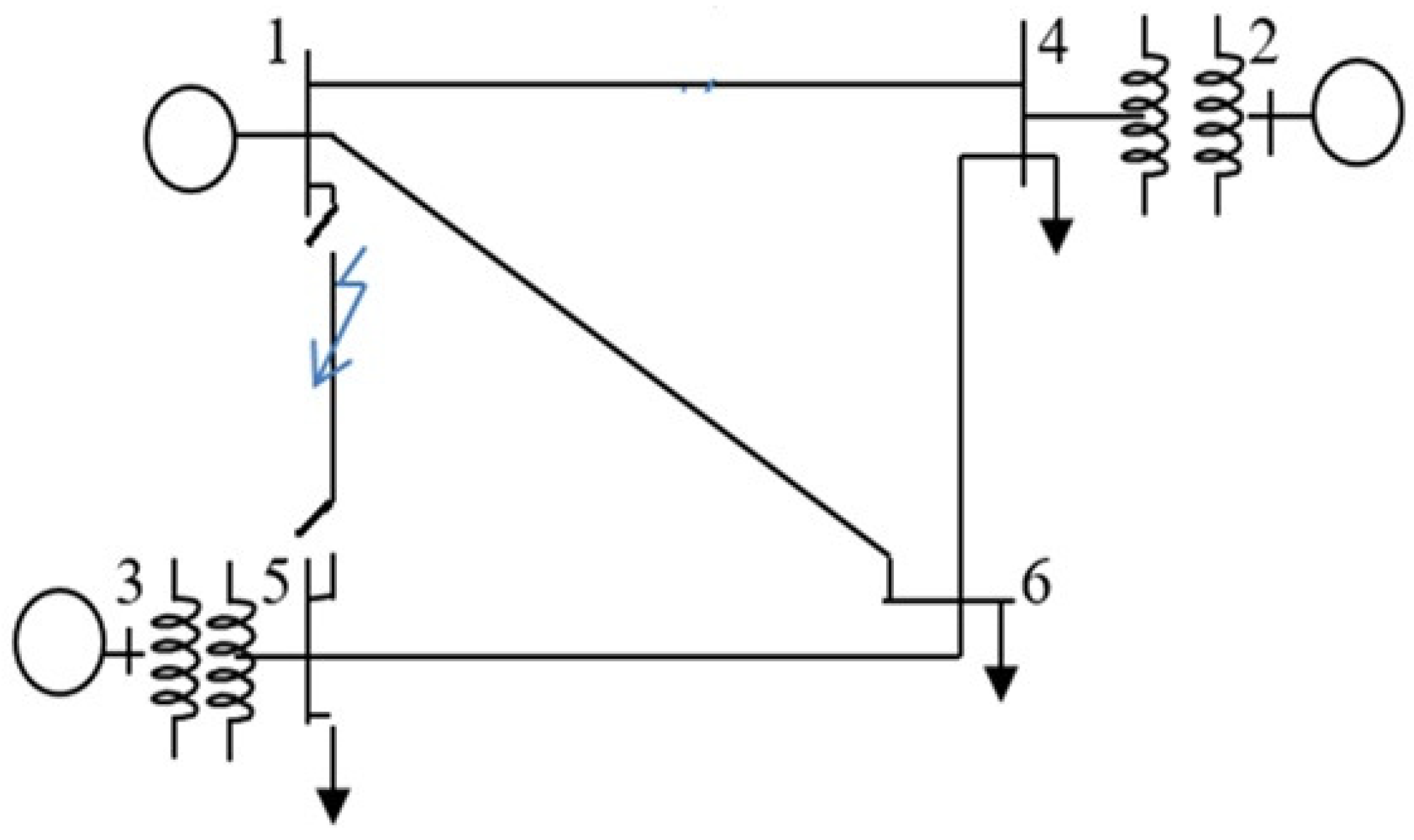
• The proposed design’s efficacy is tested on a 3-machine 6-bus power system.

1.3. Structure of the Paper

The following is a summary of the paper’s structure. Section 2 presents the problem description as a stochastic model of a multi-machine system based on stochastic calculus. In Section 3, preliminary mathematical tools of stochastic calculus to solve the stability problem are given. In Section 4, the stochastic disturbance stabilizer is designed. Numerical simulations are given in Section 5. Finally, the conclusions are presented in Section 6.

1.4. Notation

Throughout this paper,

• ${\mathbb{R}}^n$ denotes the n-dimensional Euclidean space;
• ${\mathbb{R}}^{m\times n}$ is the space of real matrices of dimension $m\times n$;
• $∥·∥$ refers to the Euclidean vector norm;
• The probability space with the sample space $\Omega ;$ $\sigma$-algebra F of subsets of the sample space, and probability measure $\mathbb{P}$ are represented by the notation $\left(\Omega ,\mathcal{F},\mathbb{P}\right)$;
• $\mathrm{E}$ signifies the expectation operator;
• For continuous-time systems, $\left\{{\eta }_t,t\ge 0\right\}$ is a time-homogeneous semi-Markov process with the right continuous trajectories and takes values in a finite set $\mathcal{N}=\left\{1,2,\dots ,N\right\}$ with stationary transition probabilities

  $$\mathbb{P}\left\{{\eta }_{t+h}=j\mid {\eta }_t=i\right\}=\left\{\begin{array}{ccc}{\pi }_{ij}h+o\left(h\right)& \mathrm{if}& i\ne j\\ 1+{\pi }_{ij}h+o\left(h\right)& \mathrm{if}& i=j\end{array}\right.$$

  (1)

  where $h>0$, $\underset{h\to 0}{lim}{\displaystyle \frac{o\left(h\right)}{h}}=0$ and ${\pi }_{ij}$ is the transition rate from mode i at time t to mode j at time $t+h$, satisfying for all $i\in \mathcal{N}$

  $${\pi }_{ii}=-\sum _{j=1,j\ne i}^N{\pi }_{ij}$$

  (2)

2. Problem Formulation

2.1. A Multi-Machine System’s Dynamic Model

Consider an $m+1$ generator multi-machine power system, where the i-th generator is connected to the other m generators.

The dynamics of m interconnected generators through a transmission network can be modeled by a classical model with flux decay dynamics [1] under some basic assumptions. The generator in this model is represented by the voltage behind direct axis transient reactance, with the voltage angle corresponding to the mechanical angle relative to the synchronously revolving reference frame. The network has been simplified to an internal bus representation, with loads assumed to be constant impedances and transfer conductance considered.

The classical third-order model [1] represents the dynamical model of the i-th machine as:

$${\dot{\delta }}_i=w_0\left(w_i-w_0\right),$$

(3)

$$\begin{array}{c}{\dot{w}}_i={\displaystyle \frac{1}{2H_i}}\left(P_{mi}-P_{ei}\right),{\dot{E}}_{qi}^{\prime }=\frac{1}{T_{d0}^{\prime }}\left(E_{fi}-E_{qi}\right)\end{array}$$

(4)

where

$$\left.\begin{array}{c}{E}_{qi}=E_{qi}^{\prime }+\left(x_{di}-x_{di}^{\prime }\right)I_{di},\Delta E_{fi}=u_i\\ P_{ei}=E_{qi}^{\prime }{\sum }_{j=1}^n{E}_{qj}^{\prime }{B}_{ij}sin\left({\delta }_i-{\delta }_j\right)\\ Q_{ei}=-E_{qi}^{\prime }{\sum }_{j=1}^n{E}_{qj}^{\prime }{B}_{ij}cos\left({\delta }_i-{\delta }_j\right)\\ I_{di}=-{\sum }_{j=1}^m{E}_{qj}^{\prime }{B}_{ij}cos\left({\delta }_i-{\delta }_j\right)\\ I_{qi}={\sum }_{j=1}^m{E}_{qj}^{\prime }{B}_{ij}sin\left({\delta }_i-{\delta }_j\right)\\ E_{qi}=V_{ti}+{\displaystyle \frac{Q_{ei}{x}_{di}}{V_{ti}}}\end{array}\right\}$$

(5)

The nomenclature specifies the notation for the multi-machine power system model. Let ${\delta }_{i0},w_0,P_{ei0}$ be the operational point for generator i. Assume $P_{mi}=\mathrm{const}$, and define $\Delta {\delta }_i:={\delta }_i-{\delta }_{i0},$ $\Delta w_i=w_i-w_{i0}$. The linearized state equation becomes for small oscillations around the operating point.

$$\dot{x}=Ax+Bu$$

(6)

where

$$\begin{array}{c}x={\left[x_1^{⊺},\dots ,x_m^{⊺}\right]}^{⊺}\in R^{n=3m}\\ x_i^{⊺}=\left[\Delta {\delta }_i,\Delta w_i,\Delta E_{qi}^{\prime }\right]\left(i=1,\dots ,m\right)\end{array}$$

(7)

Note that the linearization can be carried out numerically using the MatLab code linmod.

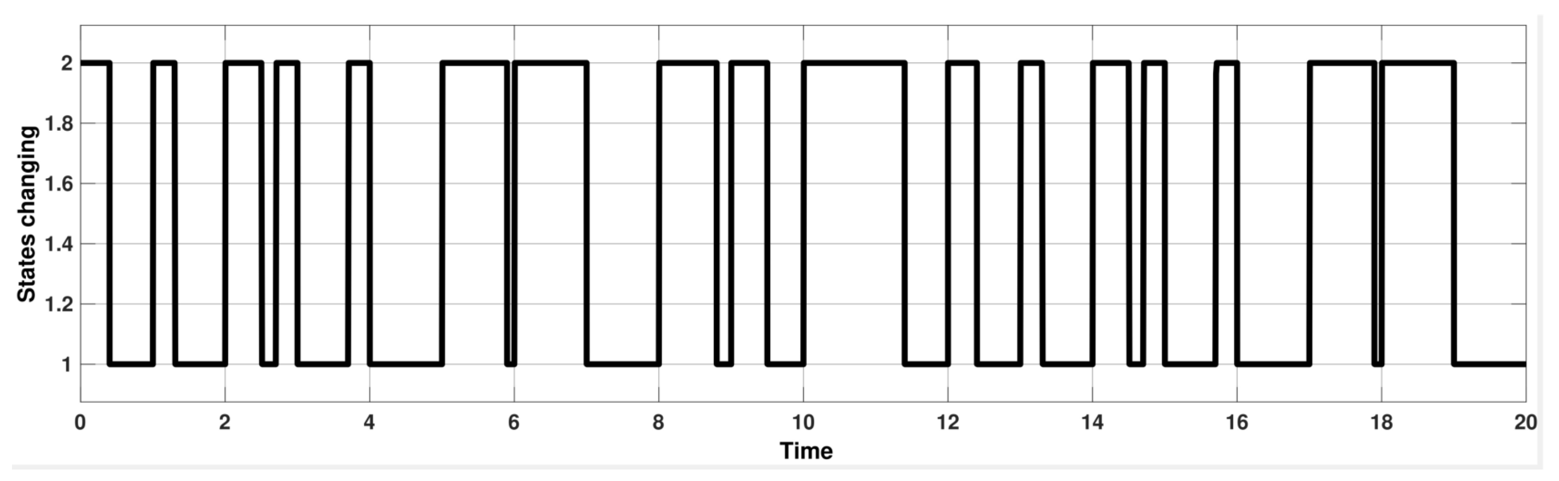
2.2. Continuous-Time Markov Model of Power System Subject to a Sequence of Lightning Strikes

Consider the multi-machine system in the case study hit by a succession of lightning strikes (see Figure 1).

We considered lightning as hitting only one line because hitting two or more lines simultaneously is very remote. We select lines 1–5 for switching because it represents one of the severe cases (generator 3 will be heavily stressed to feed its load and thus becomes nearer to instability).

Table 1. Normal loading conditions and system data.

Bus #	1	2	3	4	5	6
Gen-$Mw$		150	100
Load-$Mw$	0	0	0	100	90	160
Load-$Mvar$	0	0	0	70	30	110
$x_d,$$x_q,$$x_d^{\prime }$	0.8, 0.8, 0.2	1.3, 1.3, 0.15	0.9, 0.9, 0.25
$T_{d0}^{\prime }$	9	5.8	6
H	20	4	5
Bus #	Bus #	$\mathit{R}(\mathit{p},\mathit{u})$	$\mathit{X}(\mathit{p},\mathit{u})$	$\mathbf{0.5}\mathit{B}(\mathit{p},\mathit{u})$
1	4	0.035	0.025	0.0065
1	5	0.025	0.105	0.0045
1	6	0.04	0.215	0.0055
3	4	0	0.035	0
3	5	0	0.042	0
4	6	0.028	0.125	0.0035
5	6	0.026	0.175	0.03

shows the system’s data (see [28]).

The circuit breaker opens the line to clear the fault when a lightning strike hits the transmission line, say lines 1–5. The circuit breakers are provided with an auto-reclosure mechanism to close the line because the majority of failures are transient. When the issue persists, the auto-reclosing action is tried 1–2 times before being terminated and the line stays open (permanent).

In the simplest case, the power system dynamics under a succession of lightning strikes could be represented by an N-mode Markov jump linear system, as illustrated in Figure 1 (MJLS). Particularly, the system switches between N modes at random (due to circuit breaker open/closed in respect to a series of random lightning strikes). For our case, the number of modes N = 2. The power system dynamics can be described as a Markov jump linear system (MJLS). Hence, the line’s parameter entering the state matrix A changes in random jumps. Another change in the line’s parameter is due to the random wind speed affecting the phase conductors spacing (which in turn affects the line reactance). Similarly, the random ambient temperature changes affect the line resistance. The later effects are grouped and represented as a stochastic external disturbance (noise).

This MJLS + stochastic parameter external disturbances is represented as

$$\left.\begin{array}{c}\dot{x}\left(t\right)=A\left({\eta }_t\right)x\left(t\right)+B\left({\eta }_t\right)u\left(t\right)+\Xi \left({\eta }_t\right)w\left(t\right),\\ x\left(0\right)=x_0,\end{array}\right\}$$

(8)

where $x\left(t\right)$, $u\left(t\right)$, and $w\left(t\right)$ are the state, control, and external stochastic disturbance (noise) vectors of dimensions n, k, and l, respectively. Due to the fast, sharp changes in the slopes of the random noise, the derivative in (8) may be undefined. So, the ordinary differential Equation (8) is not suitable to model a stochastic system. It is better to cast (8) as a stochastic differential equation (SDE):

$$\left.\begin{array}{c}dx\left(t\right)=\left[A\left({\eta }_t\right)x\left(t\right)+B\left({\eta }_t\right)u\left(t\right)\right]dt+\Xi \left({\eta }_t\right)dW\left(t\right),\\ x\left(0\right)=x_0,A\left({\eta }_t\right)\in {\mathbb{R}}^{n\times n},B\left({\eta }_t\right)\in {\mathbb{R}}^{n\times k},\Xi \left({\eta }_t\right)\in {\mathbb{R}}^{n\times l}\end{array}\right\}$$

(9)

Problem 1.

The problem is to design a state feedback

$$u\left(t\right)=K\left({\eta }_t\right)x\left(t\right),K\left({\eta }_t\right)\in {\mathbb{R}}^{k\times n}$$

(10)

such that the state trajectories of the stochastic system (9) are attracted to a small region (represented by ellipsoids with minimum volumes) around the origin in a mean-square sense. A novel excitation control mechanism is applied against the stochastic uncertainties. Sufficient conditions in the form of LMIs are given where the energetic function, containing the matrix P, characterizes the “attractive ellipsoid” for the considered controlled process independently of the system mode. The matrix P cannot be dependent on the current mode of the system model since, by its physical nature, it should characterize the final effect of the applied control action independently on a varied structure of the plant. So, this reflects the contracting property of the applied control and is clearly understandable by the engineering community.

3. Problem Solution

3.1. Closed-Loop System

The closed-loop version of system (9) associated with the controller (10) is

$$\left.\begin{array}{c}dx\left(t\right)=A_K\left({\eta }_t\right)dt+\Xi \left({\eta }_t\right)dW\left(t\right),\\ x\left(0\right)=x_0,\\ A_K\left({\eta }_t\right):=A\left({\eta }_t\right)+B\left({\eta }_t\right)K\left({\eta }_t\right)\end{array}\right\}$$

(11)

3.2. Main Result

Theorem 1.

If for the linear system (11) there exist positive definite matrices $P_i$ and $Q_i$ and positive numbers ${\alpha }_i$ such that for all $i=1,\dots ,N$

$$\begin{array}{c}{W}_i:=P_i{A}_{K,i}+A_{K,i}^{⊺}{P}_i+\sum _{j=1}^N{\pi }_{ij}{P}_j+{\alpha }_i{P}_i=\\ P_i{A}_{K,i}^{\alpha }+{\left(A_{K,i}^{{}^{\alpha }}\right)}^{⊺}{P}_i+\sum _{j=1,j\ne i}^N{\pi }_{ij}{P}_j<0\end{array}$$

(12)

and

$${\Xi }_i^{⊺}{P}_i{\Xi }_i\le Q_i,$$

(13)

where

$$\begin{array}{c}{A}_{K,i}^{\alpha }=A_{K,i}+{\displaystyle \frac{{\alpha }_i+{\pi }_{ii}}{2}}{I}_{n\times n}=A_i+B_i{K}_i+{\displaystyle \frac{{\alpha }_i+{\pi }_{ii}}{2}}{I}_{n\times n},\\ A_i=A\left({\eta }_t=i\right),B_i=B\left({\eta }_t=i\right),K_i=K\left({\eta }_t=i\right),\end{array}$$

then we may guarantee the simultaneous mean-square convergence of trajectories $x\left(t\right)$ to the attractive ellipsoids ${\mathcal{E}}_i\left(P_{i,attr}\right)$, that is,

$$\left.\begin{array}{c}\underset{t\to \infty }{lim\; sup}\mathrm{E}\left\{x^{⊺}\left(t\right)P_{i,attr}x\left(t\right)\right\}\le 1,\\ \\ P_{i,attr}={\displaystyle \frac{{\alpha }_i}{\mathrm{tr}{Q}_i}}{P}_i,i=1,\dots ,N,\end{array}\right\}$$

(14)

providing the mean-square convergence of all trajectories ${\left\{x\left(t\right)\right\}}_{t\ge 0}$ to the intersections $\mathcal{E}$ of all ellipsoids ${\mathcal{E}}_i\left(P_{i,attr}\right)$ (which is in fact not an ellipsoid), namely,

$$\begin{array}{c}x\left(t\right)\underset{t\to \infty }{\stackrel{l.i.m.}{\to }}\mathcal{E},\mathcal{E}=\underset{i=1,\dots ,N}{\cap }{\mathcal{E}}_i\left(P_{i,attr}\right),\end{array}$$

where

$${\mathcal{E}}_i\left(P_{i,attr}\right):=\left\{x\in {\mathbb{R}}^n:x^{⊺}{P}_{i,attr}x\le 1\right\}.$$

Proof. 

It follows directly from Theorem A1 and Corollary A1 (see Appendix A.4). □

4. Optimal Feedback Gain Selection

A novel excitation control mechanism is applied against the stochastic uncertainties. Sufficient conditions in the form of LMIs are given where the energetic function, containing the matrix P, characterizes the “attractive ellipsoid” for the considered controlled process independently of the system mode. The matrix P cannot be dependent on the current mode of the system model since, by its physical nature, it should characterize the final effect of the applied control action independently on a varied structure of the plant. So, this reflects the contracting property of the applied control and is clearly understandable by the engineering community.

4.1. Optimization Problem Formulation

Optimal selection of the gain parameters $K_i$ $\left(i=1,\dots ,N\right)$ consists in finding positive definite matrices $P_i$ and $Q_i,$ matrices $K_i$, and positive numbers ${\alpha }_i$, which are the solutions of the following optimization problem

$$\sum _{i=1}^N\mathrm{tr}{P}_{i,attr}=\sum _{i=1}^N{\displaystyle \frac{{\alpha }_i}{\mathrm{tr}{Q}_i}}\mathrm{tr}{P}_i\to \underset{0<P_i,0<Q_i,K_i,0<{\alpha }_i,}{sup}$$

or equivalently,

$$\sum _{i=1}^N\mathrm{tr}{P}_{i,attr}^{-1}=\sum _{i=1}^N{\displaystyle \frac{\mathrm{tr}{Q}_i}{{\alpha }_i}}\mathrm{tr}{P}_i^{-1}\to \underset{0<P_i,0<Q_i,K_i,0<{\alpha }_i,}{inf}$$

(15)

subject to the system of nonlinear matrix inequalities (NMIs)

$$\left.\begin{array}{c}{W}_i:=P_i\left(A_i+B_i{K}_i+{\displaystyle \frac{{\alpha }_i+{\pi }_{ii}}{2}}{I}_{n\times n}\right)+{\left(A_i+B_i{K}_i+{\displaystyle \frac{{\alpha }_i+{\pi }_{ii}}{2}}{I}_{n\times n}\right)}^{⊺}{P}_i\\ +{\sum }_{j=1,j\ne i}^N{\pi }_{ij}{P}_j<0\\ \\ {\Xi }_i^{⊺}{P}_i{\Xi }_i\le Q_i\left(i=1,\dots ,N\right).\end{array}\right\}$$

(16)

4.2. Transformation of the Optimization Problems under MNIs Constrains to the Problem with LMIs

(a) Using Schur’s complement lemma, the inequalities ${\Xi }_i^{⊺}{P}_i{\Xi }_i\le Q_i$ can be equivalently represented as

$$\left[\begin{array}{cc}{Q}_i& {\Xi }_i\\ {\Xi }_i^{⊺}& P_i^{-1}\end{array}\right]\ge 0\left(i=1,\dots ,N\right)$$

(17)

(b) Notice that $W_i<0$ if and only if ${\left(P_i^{-1}\right)}^{⊺}{W}_i{P}_i^{-1}<0,$ which leads to

$$\begin{array}{c}{\left(P_i^{-1}\right)}^{⊺}{W}_i{P}_i^{-1}:=\left(A_i+B_i{K}_i+{\displaystyle \frac{{\alpha }_i+{\pi }_{ii}}{2}}{I}_{n\times n}\right)P_i^{-1}+\\ {\left(P_i^{-1}\right)}^{⊺}{\left(A_i+B_i{K}_i+{\displaystyle \frac{{\alpha }_i+{\pi }_{ii}}{2}}{I}_{n\times n}\right)}^{⊺}+{\sum }_{j=1,j\ne i}^N{\pi }_{ij}\left[{\left(P_i^{-1}\right)}^{⊺}{P}_j{P}_i^{-1}\right]<0,\end{array}$$

(18)

Using the estimates

$$\left[{\left(P_i^{-1}\right)}^{⊺}{P}_j{P}_i^{-1}\right]\le S_{ij}$$

(19)

for some positive definite matrices $S_i$ and Schur’s complement lemma for (19)

$$\left[\begin{array}{cc}{S}_{ij}& P_i^{-1}\\ {\left(P_i^{-1}\right)}^{⊺}& P_j^{-1}\end{array}\right]\ge 0\left(i=1,\dots ,N\right),$$

(20)

we are able to represent the nonlinear system of matrix inequalities (18) as the corresponding system of LMIs that gives

$$\begin{array}{c}{A}_{K,i}^{\alpha }{X}_i+X_i{\left(A_{K,i}^{\alpha }\right)}^{⊺}+B_i{Y}_i+{\left(Y_i\right)}^{⊺}{B}_i^{⊺}+{\sum }_{j=1,j\ne i}^N{\pi }_{ij}{S}_{ij}<0\\ \left[\begin{array}{cc}{Q}_i& {\Xi }_i\\ {\Xi }_i^{⊺}& X_i\end{array}\right]\ge 0,\\ \left[\begin{array}{cc}{S}_{ij}& X_i\\ {\left(X_i\right)}^{⊺}& X_j\end{array}\right]\ge 0\left(j\ne i=1,\dots ,N\right),\end{array}$$

(21)

where

$$X_i:=P_i^{-1},Y_i:=K_i{P}_i^{-1}.$$

(22)

The main result of this paper follows.

Theorem 2.

The optimization problem (15) under the NMIs (nonlinear matrix inequalities) constraints (16) are equivalent to the following optimization problem

$$\sum _{i=1}^N{\displaystyle \frac{\mathrm{tr}{Q}_i}{{\alpha }_i}}\mathrm{tr}{X}_i\to \underset{0<X_i,0<Q_i,Y_i,0<S_{ij}0<{\alpha }_i,}{inf}$$

(23)

subject to the system of LMIs (21). The feedback control gain matrices $K_i^{*}$, minimizing the “size” of the attractive ellipsoids are

$$K_i^{*}=Y_i^{*}{\left(X_i^{*}\right)}^{-1},i=1,2.$$

(24)

5. Numerical Example

The numerical simulations are carried out using the following system parameters:

• The example below is solved numerically for $N=2$,

  $$\left[{\pi }_{ij}\right]:=\left[\begin{array}{cc}{\pi }_{11}=-0.8& {\pi }_{12}=0.8\\ {\pi }_{21}=0.1& {\pi }_{22}=-0.1\end{array}\right]$$

$$\begin{array}{c}{\Xi }_1:={\left[\begin{array}{cccccc}0.2& 0.1& 0.1& 0.3& 0.2& 0.3\end{array}\right]}^{⊺}\\ {\Xi }_2:={\left[\begin{array}{cccccc}0.1& 0.2& 0.2& 0.3& 0.1& 0.3\end{array}\right]}^{⊺}\end{array}$$

with the initial conditions (caused by a cleared fault):

$$x\left(0\right)={\left[\begin{array}{cccccc}0.3& 0& 0& 0.1& 0& 0\end{array}\right]}^{⊺}$$

Mode 1 (Lines 1–5 Connected, No Fault)

$$A_1=\left[\begin{array}{cccccc}0& 377& 0& 0& 0& 0\\ -0.335& 0& -0.347& 0.0115& 0& 0.0463\\ -0.463& 0& -0.870& 0.0204& 0& 0.0275\\ 0& 0& 0& 0& 377& 0\\ -0.152& 0& 0.00372& -0.1919& 0& -0.1834\\ 0.0122& 0& 0.0168& -0.1786& 0& -0.4645\end{array}\right]$$

$$B_1^{⊺}=\left[\begin{array}{cccccc}0& 0& 0.1724& 0& 0& 0\\ 0& 0& 0& 0& 0& 0.1667\end{array}\right]$$

Mode 2 (Lines 1–5 Disconnected Due to Fault)

$$A_2=\left[\begin{array}{cccccc}0& 377& 0& 0& 0& 0\\ -0.3269& 0& -0.3415& 0.03326& 0& 0.0006889\\ -0.4445& 0& -0.8632& 0.0561& 0& 0.05124\\ 0& 0& 0& 0& 377& 0\\ 0.02448& 0& 0.008583& -0.139& 0& -0.152\\ 0.02544& 0& 0.03866& -0.9945& 0& -0.377\end{array}\right],$$

$$B_2^{⊺}=\left[\begin{array}{cccccc}0& 0& 0.1724& 0& 0& 0\\ 0& 0& 0& 0& 0& 0.1667\end{array}\right]$$

5.1. Optimal Parameters

Applying the matrix optimization procedure (23) and the relations (24), we obtained the following results:

$${\alpha }_1^{*}=0.4211,{\alpha }_2^{*}=0.2210,$$

$$\begin{array}{c}{P}_1^{*}={10}^{+5}·\mathrm{Inv}\left(X_1\right)\\ P_1^{*}=\left[\begin{array}{cccccc}753.12& 15,173.79& -10.30& 243.49& 2124.15& -2.53\\ 15,173.79& 337,027.17& -225.35& 2311.34& -22,769.64& -38.38\\ -10.30& -225.35& 1.71& -0.23& 47.67& 0.55\\ 243.49& 2311.34& -0.23& -232.70& -6972.22& 2.17\\ 2124.15& -22,769.64& 47.67& -6972.22& -130,245.04& 54.47\\ -2.53& -38.38& 0.55& 2.17& 54.47& 1.21\end{array}\right]\end{array}$$

$$\begin{array}{c}{P}_2^{*}={10}^{+5}·\mathrm{Inv}\left(X_1\right)\\ P_2^{*}=\left[\begin{array}{cccccc}100.39& -712.52& 0.69& -109.33& -4343.40& 1.27\\ -712.52& 115,383.84& -71.57& 5489.50& 166,495.64& -60.23\\ 0.69& -71.57& 0.181& -3.67& -115.00& 0.058\\ -109.33& 5489.50& -3.67& 379.45& 12,161.87& -3.99\\ -4343.40& 166,495.64& -115.00& 12,161.87& 432,852.67& -137.70\\ 1.27& -60.23& 0.058& -3.99& -137.70& 0.21\end{array}\right]\end{array}$$

$$\begin{array}{c}{K}_1^{*}=\left[\begin{array}{cccccc}781.9& 3981.2& -1461.6& -561.6& -3412.8& 673.2\\ 662.4& 112& 696.6& -276.5& 781.6& -1976\end{array}\right],\\ K_2^{*}=\left[\begin{array}{cccccc}743& 23,662& -1978& -964& -21,977& 514\\ 1032& -21,318& 530& 392& 21,200& -1836\end{array}\right],\end{array}$$

(25)

$$\mathrm{tr}\left(Q_1^{*}\right)={10}^{+5}·\left(1.9924\right),\mathrm{tr}\left(Q_2^{*}\right)={10}^{+5}·\left(1.9832\right)$$

$$\begin{array}{c}\mathrm{tr}{P}_{1,attr}={\displaystyle \frac{{\alpha }_1^{*}}{\mathrm{tr}{Q}_1^{*}}}\mathrm{tr}{P}_1^{*}={10}^4·\left(4.1620\right),\\ \mathrm{tr}{P}_{2,attr}={\displaystyle \frac{{\alpha }_2^{*}}{\mathrm{tr}{Q}_2^{*}}}\mathrm{tr}{P}_2^{*}={10}^4·\left(5.508\right).\end{array}$$

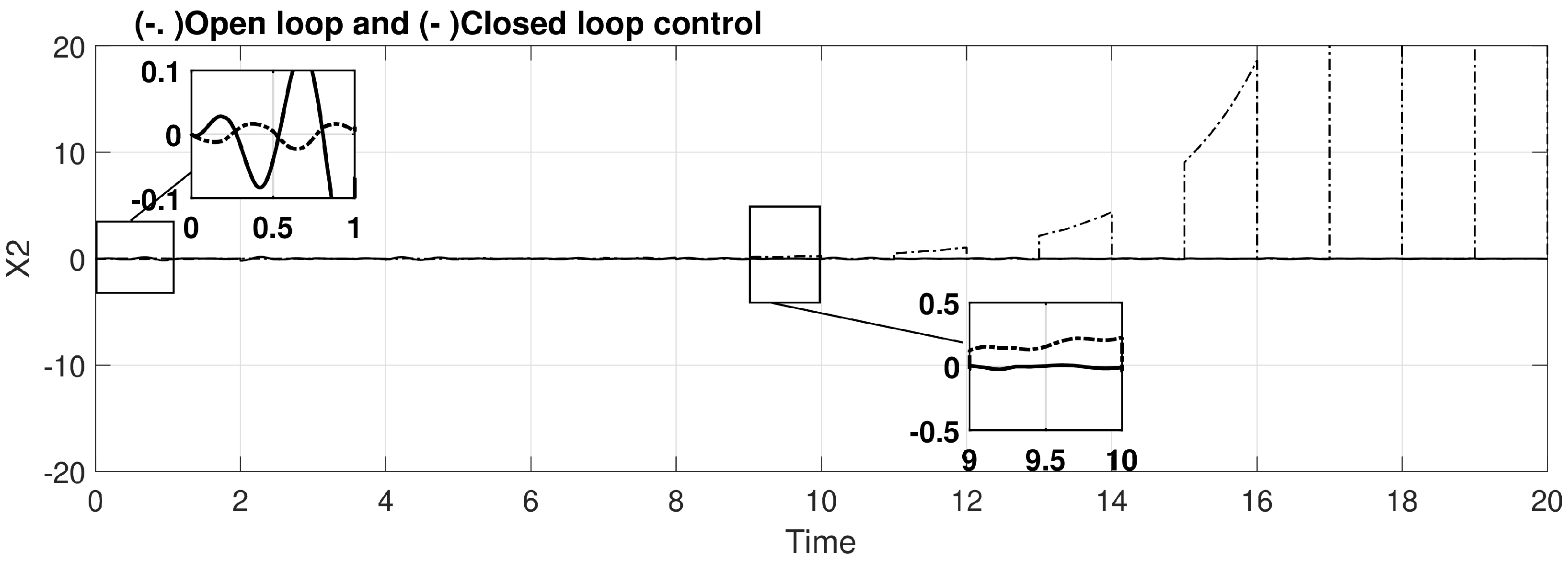
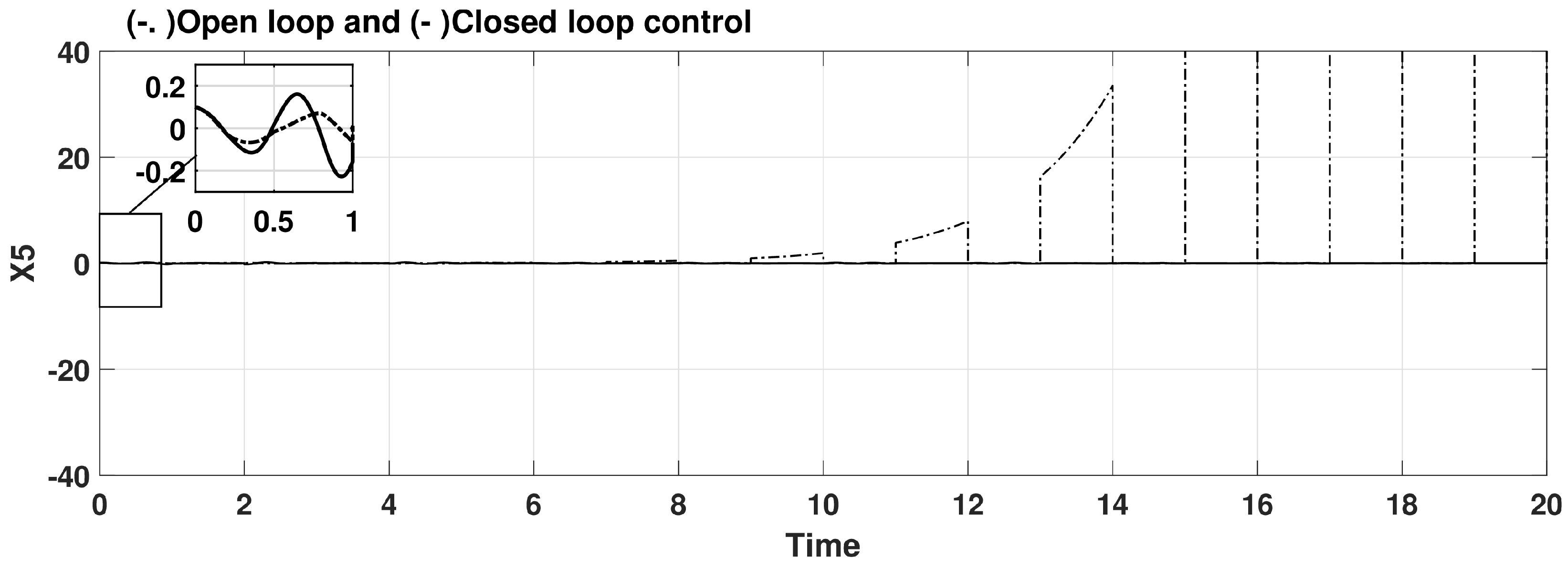
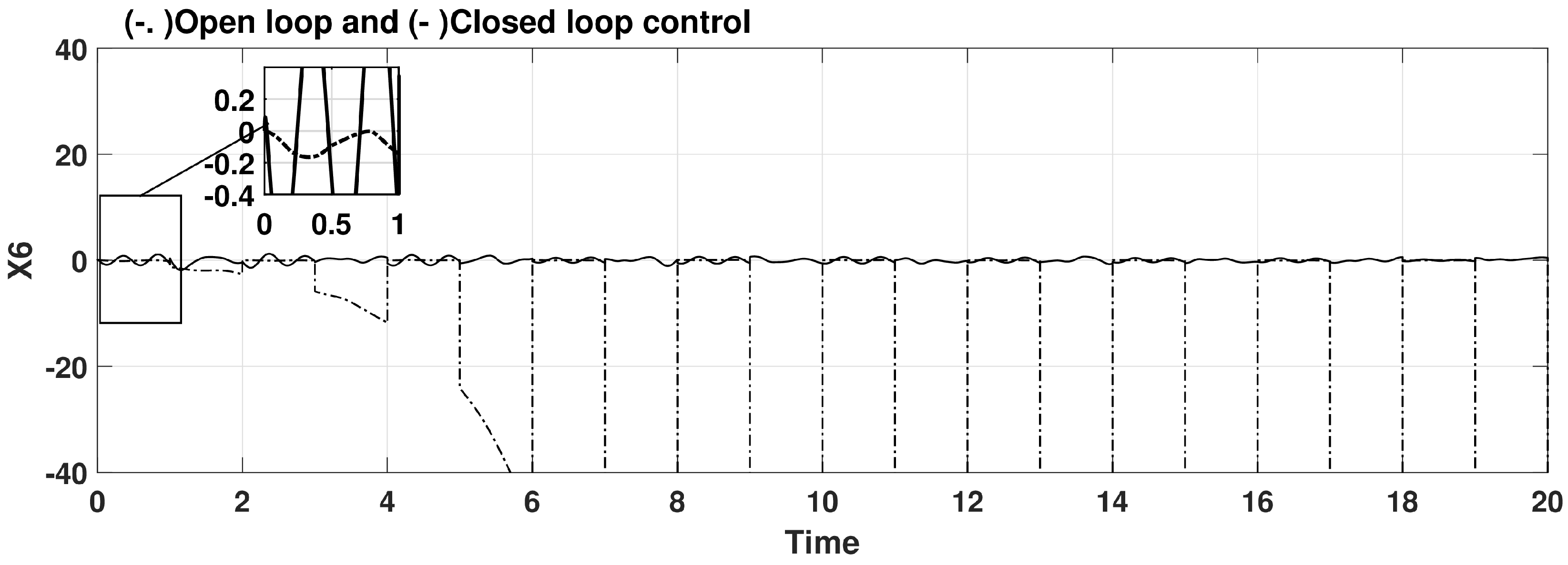
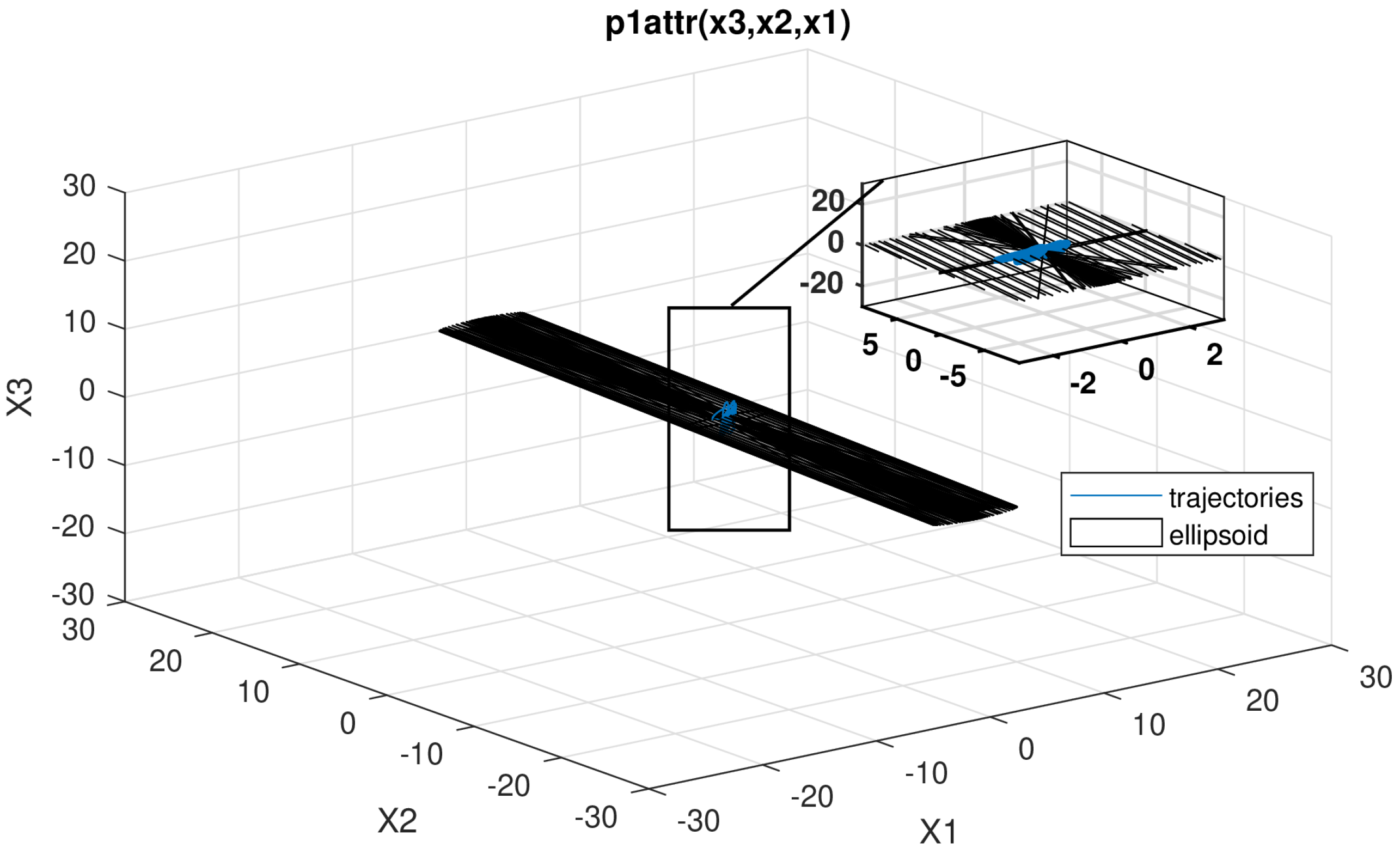
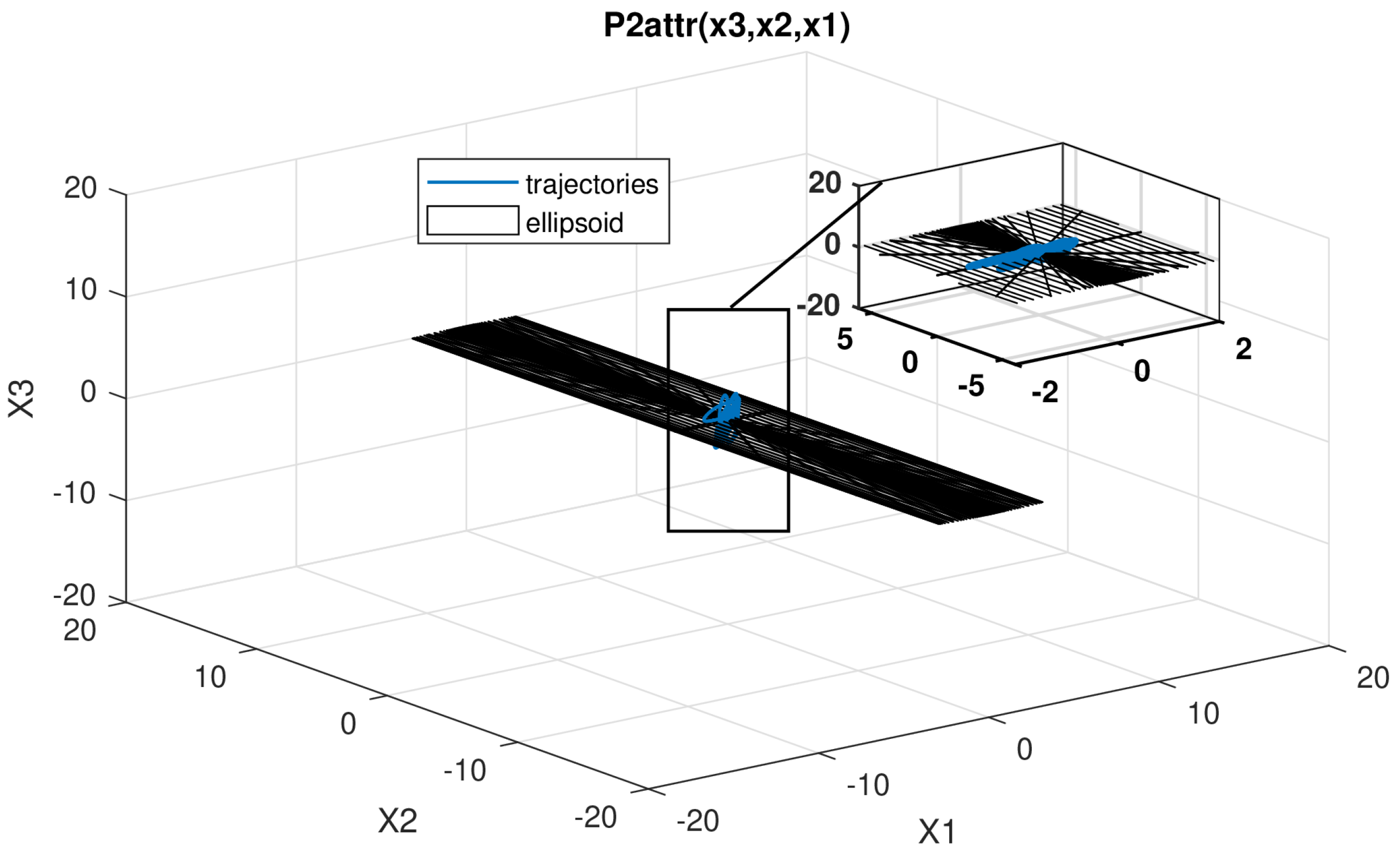
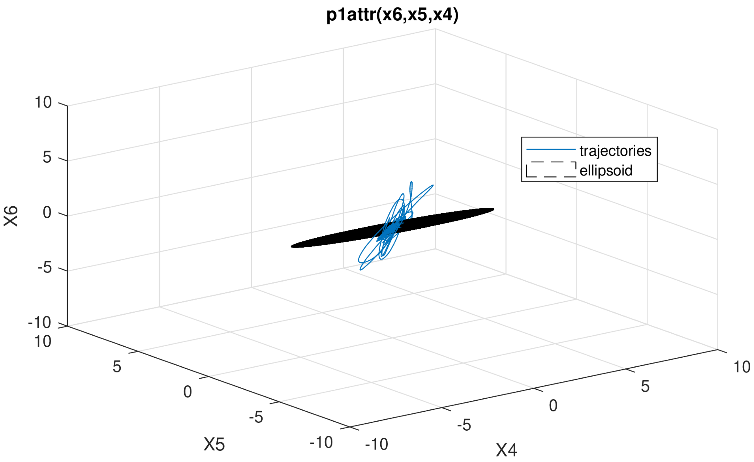
5.2. Illustrating Figures

Figure 2, Figure 3, Figure 4, Figure 5, Figure 6, Figure 7, Figure 8, Figure 9, Figure 10, Figure 11 and Figure 12 depict the behavior without (shown as -.-.) and with the proposed control (shown as -). As seen, the open-loop response is unstable, whereas the proposed control stabilizes well the system in a mean-square sense under the optimal parameters (25).

The above figures show that the system without control is unstable, whereas the proposed controller succeeds in stabilizing the system effectively.

6. Conclusions

For a stochastic power system, this work proposes a new robust excitation control of rotor angle stabilization (in a mean-square sense). A stochastic dynamic model is derived for a multi-machine test system subject to stochastic factors (random topological and parameter changes). The system subject to a series of lightning strikes associated with auto-reclosures of circuit breakers is modeled by continuous-time Markov jumps. The random parameter changes in the system are represented by external disturbances. A sufficient condition is derived as a set of nonlinear matrix inequalities (transformed into LMIs) for the proposed control. The condition is derived using the invariant ellipsoid method. The ellipsoid’s volume is minimized to achieve the optimal performance of the system. On a multi-machine system, the effectiveness of the suggested control is assessed. It damps well the system’s oscillations in a mean-square sense. The future study is to include packet loss and delays in communication networks used in power grids.

References

1. Machowski, J.; Lubosny, Z.; Bialek, J.W.; Bumby, J.R. Power System Dynamics: Stability and Control; John Wiley&Sons: Croydon, UK, 2020. [Google Scholar]
2. El-Sheikhi, F.A.; Soliman, H.M.; Ahshan, R.; Hossain, E. Regional pole placers of power systems under random failures/repair Markov jumps. Energies 2021, 14, 1989. [Google Scholar] [CrossRef]
3. Soliman, H.M.; Elshafei, A.L.; Shaltout, A.A.; Morsi, M.F. Robust power system stabilizer. IEE Proc. Gener. Distrib. 2000, 147, 285–291. [Google Scholar] [CrossRef]
4. Soliman, H.M.; Dabroum, A.; Mahmoud, M.S.; Soliman, M. Guaranteed-cost reliable control with regional pole placement of a power system. J. Frankl. Inst. 2011, 348, 884–898. [Google Scholar] [CrossRef]
5. Derbel, N.; Ghommam, J.; Zhu, Q. Diagnosis, Fault Detection & Tolerant Control; Springer: Berlin/Heidelberg, Germany, 2020. [Google Scholar]
6. Soliman, H.M.; Yousef, H.A. Saturated robust power system stabilizers. Int. J. Electr. Power Energy Syst. 2015, 73, 608–614. [Google Scholar] [CrossRef]
7. Yousef, H.; Soliman, H.M.; Albadi, M. Nonlinear power system excitation control using adaptive wavelet networks. Neurocomputing 2017, 30, 302–311. [Google Scholar] [CrossRef]
8. Soliman, H.M.; El Metwally, K.A. Robust pole placement for power systems using two-dimensional membership fuzzy constrained controllers. IET Gener. Transm. Distrib. 2017, 11, 3966–3973. [Google Scholar] [CrossRef]
9. Soliman, M.; Elshafei, A.L.; Bendary, F.; Mansour, W. Robust decentralized PID-based power system stabilizer design using an ILMI approach. Electr. Power Syst. Res. 2008, 80, 1488–1497. [Google Scholar] [CrossRef]
10. Soliman, M. Robust non-fragile power system stabilizer. Int. J. Electr. Power Energy Syst. 2015, 64, 626–634. [Google Scholar] [CrossRef]
11. Soliman, M. Parameterization of robust three-term power system stabilizers. Electr. Power Syst. Res. 2014, 17, 172–184. [Google Scholar] [CrossRef]
12. Nwankpa, C.O.; Shahidehpour, S.M.; Schuss, Z.A. stochastic approach to small disturbance stability analysis. IEEE Trans. Power Syst. 1992, 7, 1519–1528. [Google Scholar] [CrossRef]
13. Rueda, J.L.; Colome, D.G.; Erlich, I. Assessment and enhancement of small signal stability considering uncertainties. IEEE Trans. Power Syst. 2009, 24, 198–207. [Google Scholar] [CrossRef]
14. Chung, C.Y.; Wang, K.W.; Tse, C.T.; Bian, X.Y.; David, A.K. Probabilistic eigenvalue sensitivity analysis and PSS design in multimachine systems. IEEE Trans. Power Syst. 2003, 18, 1439–1445. [Google Scholar] [CrossRef]
15. Ugrinovskii, V.; Pota, H.R. Decentralized control of power systems via robust control of uncertain Markov jump parameter systems. Int. J. Control. 2005, 78, 662–677. [Google Scholar] [CrossRef]
16. Ma, J.; Wang, S.; Qiu, Y.; Li, Y.; Wang, Z.; Thorp, J.S. Angle stability analysis of power system with multiple operating conditions considering cascading failure. IEEE Trans. Power Systems 2017, 32, 873–882. [Google Scholar] [CrossRef]
17. Soliman, H.; Shafiq, M. Robust stabilisation of power systems with random abrupt changes. IET Gener. Distrib. 2015, 9, 2159–2166. [Google Scholar] [CrossRef]
18. Ju, P. Fundamentals of Stochastic Dynamics. In Stochastic Dynamics of Power Systems; Springer: Singapore, 2019. [Google Scholar]
19. Duffy, D.G. Advanced Engineering Mathematics with MATLAB®, 3rd ed.; Chapman and Hall/CRC: New York, NY, USA, 2016. [Google Scholar]
20. Yuan, B.; Zhou, M.; Li, G.; Zhang, X.P. Stochastic small-signal stability of power systems with wind power generation. IEEE Trans. Power Syst. 2014, 30, 1680–1689. [Google Scholar] [CrossRef]
21. Sun, Y.; Wang, Y.; Wei, Z.; Sun, G.; Wu, X. Robust H load frequency control of multi-area power system with time delay: A sliding mode control approach. IEEE/CAA J. Autom. 2017, 5, 610–617. [Google Scholar] [CrossRef]
22. Zhang, Z.; Liu, Y. Stochastic Small Signal Interval Stability of Power Systems with Asynchronous Wind Turbine Generators. Math. Probl. Eng. 2018, 2018, 7617394. [Google Scholar] [CrossRef]
23. Kuppusamy, S.; Joo, Y.H.; Kim, H.S. Asynchronous Control for Discrete-Time Hidden Markov Jump Power Systems. IEEE Trans. Cybern. 2021, 52, 9943–9948. [Google Scholar] [CrossRef]
24. Soliman, H.M.; Alazki, H.; Poznyak, A.S. Robust stabilization of power systems subject to a series of lightning strokes modeled by Markov jumps: Attracting ellipsoids approach. J. Frankl. Inst. 2022, 35, 3389–3404. [Google Scholar] [CrossRef]
25. Poznyak, A.S.; Alazki, H.; Soliman, H.M. Invariant-set design of observer-based robust control for power systems under stochastic topology and parameters changes. Int. J. Electr. Power Energy Syst. 2016, 131, 107–112. [Google Scholar] [CrossRef]
26. Poznyak, A.; Polyakov, A.; Azhmyakov, V. Attractive Ellipsoids in Robust Control; Birkhauser: Boston, MA, USA, 2014. [Google Scholar]
27. Alazki, H.; Hernández, E.; Ibarra, J.; Poznyak, A. Attractive ellipsoid method controller under noised measurements for SLAM. Int. Control. Autom. Syst. 2017, 15, 2764–2775. [Google Scholar] [CrossRef]
28. Saadat, H. The Power System and Electric Power Generation, 3rd ed.; PSA Publishing: Alexandria, VA, USA, 2010; pp. 154–196. [Google Scholar]
29. Feng, X.; Loparo, K.A.; Ji, Y.; Chizeck, H.J. Stochastic stability properties of jump linear systems. IEEE Trans. Automatic Control. 1992, 37, 38–53. [Google Scholar] [CrossRef]
30. Hou, Z.; Luo, J.; Shi, P.; Nguang, S.K. Stochastic stability of Ito differential equations with semi-Markovian jump parameters. IEEE Trans. Autom. Control. 2006, 51, 1383–1387. [Google Scholar] [CrossRef]
31. Khasminskii, R. Stochastic Stability of Differential Equations; Springer Science and Business Media: Berlin/Heidelberg, Germany, 2012. [Google Scholar]
Figure 1. Lighting strikes are applied to a multi-machine system: one-line diagram of a 6-bus 3-machine system.
Energies 16 00414 g001
Figure 2. Changing states.
Energies 16 00414 g002
Figure 3. Coordinate x 1 .
Energies 16 00414 g003
Figure 4. Coordinate x 2 .
Energies 16 00414 g004
Figure 5. Coordinate x 3 .
Energies 16 00414 g005
Figure 6. Coordinate x 4 .
Energies 16 00414 g006
Figure 7. Coordinate x 5 .
Energies 16 00414 g007
Figure 8. Coordinate x 6 .
Energies 16 00414 g008
Figure 9. Convergence of x 1 ; x 2 ; x 3 in the ellipsoid P 1 a t t r .
Energies 16 00414 g009
Figure 10. Convergence of x 1 ; x 2 ; x 3 in the ellipsoid P 2 a t t r .
Energies 16 00414 g010
Figure 11. Convergence of x 4 ; x 5 ; x 6 in the ellipsoid P 1 a t t r .
Energies 16 00414 g011
Figure 12. Convergence of x 4 ; x 5 ; x 6 in the ellipsoid P 2 a t t r .
Energies 16 00414 g012