Experimental Investigation on the Vector Characteristics of Concentrated Solar Radiation Flux Map

Abstract

It is difficult to measure the concentrated solar radiation flux (CSRF) inside a cavity receiver directly due to the complex geometry of cavity receivers. At present, most reports measure the CSRF at the aperture plane (generally coinciding with the focal plane of solar concentrators) of the cavity receiver instead of at the absorber wall, which would result in serious aberration because of the obvious difference in configuration between the aperture plane and the absorber wall. To obtain the CSRF at the absorber wall with complex geometry, the vector characteristics (consisting of both directional distributions and spatial distributions) of the CSRF at the focal plane were measured using developed double water-cooled Lambertian targets together with a CCD (charge-coupled device) camera. Then the CSRF images at the absorber wall of a hemisphere cavity receiver were carried out by applying MCRTM (Monte Carlo ray-tracing method) in combination with the measured vector results of the CSRF at the aperture plane. Results show that the directional distributions of the CSRF at the aperture plane are rather nonhomogeneous along the zenith angle and the circumferential angle. The directional distribution performance of the CSRF at the focal plane plays an equally important role in the CSRF images of the cavity receivers. In addition, the relative error of the peak CSRF value of the cavity receiver between the uniform and the measured directional distribution cases is up to 16%. The conclusions provide an important reference for the development of the CSRF measurement.

1. Introduction

In high-temperature solar thermal applications, concentrated solar radiation flux (CSRF) heats solar absorbers and heat energy is transferred to the internal energy of the working fluid by convection heat transfer [1,2]. Generally, for cavity tubular receivers, the CSRF determines the heat transfer process by thermal boundary conditions. However, for volumetric receivers, the CSRF dominates the solar thermal conversion efficiency in the form of an internal heat source [3,4].

During the past few decades, the CSRF was fully investigated and discussed using both the direct measurement [5,6,7] and the indirect measurement [8,9,10,11,12]. The direct measurement method measures the CSRF at the focal plane of the solar concentrator by the movable heat flux meter or heat flux meter array. Ballestrín et al. [5] presented a direct heat flux measurement system to measure the concentrated solar power delivered by a heliostat field onto the flat aperture of solar central receiver prototypes, and the concentrated solar power and the spatial heat flux distribution have been determined by the measurement system. To avoid moving parts and allow continuous measurement, Roger et al. [6] proposed a direct method which measures the solar flux density directly on receiver surfaces and a proper scientific evaluation was discussed on the basis of specific reflectance properties of the receiver materials. Wang et al. [7] developed a new measurement method to measure the non-uniform solar flux distribution of parabolic trough collectors using a rotating heat flux gage system.

On the other hand, the indirect measurement measures heat flux distribution using a water-cooled white bar as a target and a CCD (charge-coupled device) camera to take images. The heat flux distributions are estimated by the gray image of the CCD camera together with its convert expression. Ulmer et al. [8] proposed a flux density measuring system to measure the concentrated solar radiation in the entrance aperture of solar tower receivers using a white rotating bar as a target and a CCD camera taking images. An indirect measurement apparatus was developed by Krueger K R et al. [9] to test the operational performance of a high-flux solar simulator with 45 kW power. Li et al. [10] also performed an indirect measurement experiment to predict the optical analysis of a hexagonal 42 kW high-flux solar simulator. The flux mapping method was used to evaluate the performance of an adjustable flux solar simulator for solar thermal, thermochemical and photovoltaic applications [11]. Levêque G et al. [12] conducted an experimental and numerical characterization of a new 45 kW multisource high-flux solar simulator. Compared with the direct measurement, the indirect measurement method has been widely used for its higher spatial resolution and large measuring range [13].

To decrease systematic errors, a hybrid method that consists of the direct measurement and the indirect measurement has been adopted. Ballestrín [14] designed, built and mounted a hybrid heat flux measurement system on top of the SSPS-CRS to measure the incident solar power. The two measurements are compared in detail showing a good level of agreement. To evaluate the performance of a multi-lamp high-flux solar simulator, Xiao et al. [15,16] developed a novel flux mapping system that was made up of a stationary water-cooled Lambertian target where there was a circular hole in the center used to install a flux sensor and a movable Lambertian target used to cover the flux sensor when shooting the concentrated light beam image.

However, the CSRF is a radiant vector, which is a function of both spatial coordinates and direction angles [17,18]. The above-mentioned literature mainly focused on the spatial distribution of the CSRF at the focal plane. There is a lack of experimental discussion on the directional performances of the CSRF. For simplification, most reports suppose that the directional radiative intensity is uniform for the heat transfer model of solar receivers [19,20]. Because of the complex configuration of the solar concentrating systems (e.g., heliostats field, multi-faceted dish concentrator), the radiative intensity of the CSRF is not uniform but changes with the zenith angle and the circumferential angle evidently [21,22]. The hypothesis that the radiative intensity of the CSRF is uniform will produce several disadvantages.

(i) For cavity receivers, because of the different geometric shapes between the aperture and the tubular absorbers, the spatial distributions of the CSRF measured at the aperture are quite distinct from those of the tubular absorbers [23,24,25]. More accurate thermal conditions of the tubular absorbers inside the cavity receivers could be predicted experimentally when we measure the spatial distributions together with the directional distributions of the CSRF at the aperture or the focal plane simultaneously. For volumetric receivers, the CSRF could continually transmit inside the porous absorber to form the internal heat source because the porous material is full of open cells [26,27]. A more accurate internal heat source could be obtained with both the spatial distributions and the directional distributions of the CSRF than with only single spatial distributions.

(ii) The directional distributions of the CSRF are beneficial to the optimization of the window configurations of the receiver and the compound parabolic concentrator installed at the aperture of the receiver, where the transmissivity of the CSRF depends on the angle measured between the incident direction of the sunlight and the normal direction of the window surface or compound parabolic concentrator surface [28,29,30].

(iii) To some extent, the directional radiative intensity of the CSRF represents the capacity of the solar radiation collected at the corresponding direction of the solar concentrating systems. Therefore, the directional distributions of the CSRF are useful to design and monitor solar concentrating systems [31,32].

Therefore, the directional distributions of the CSRF are of equal importance as spatial distributions for solar thermal applications. The aim of this study is to propose an experimental method to measure the directional distributions of the CSRF at the focal plane and to predict the CSRF images of cavity receivers as a function of directional distribution conditions. The article structure is as follows: in Section 2, the experimental method and apparatus are described; in Section 3, the MCRTM method coupled with experimental CSRF are given; in Section 4, the experimental results of directional distributions are presented and a case study is conducted to analyze the influence of the directional distributions on the CSRF images of the cavity receiver. Finally, the conclusions are presented.

2. Experimental Details

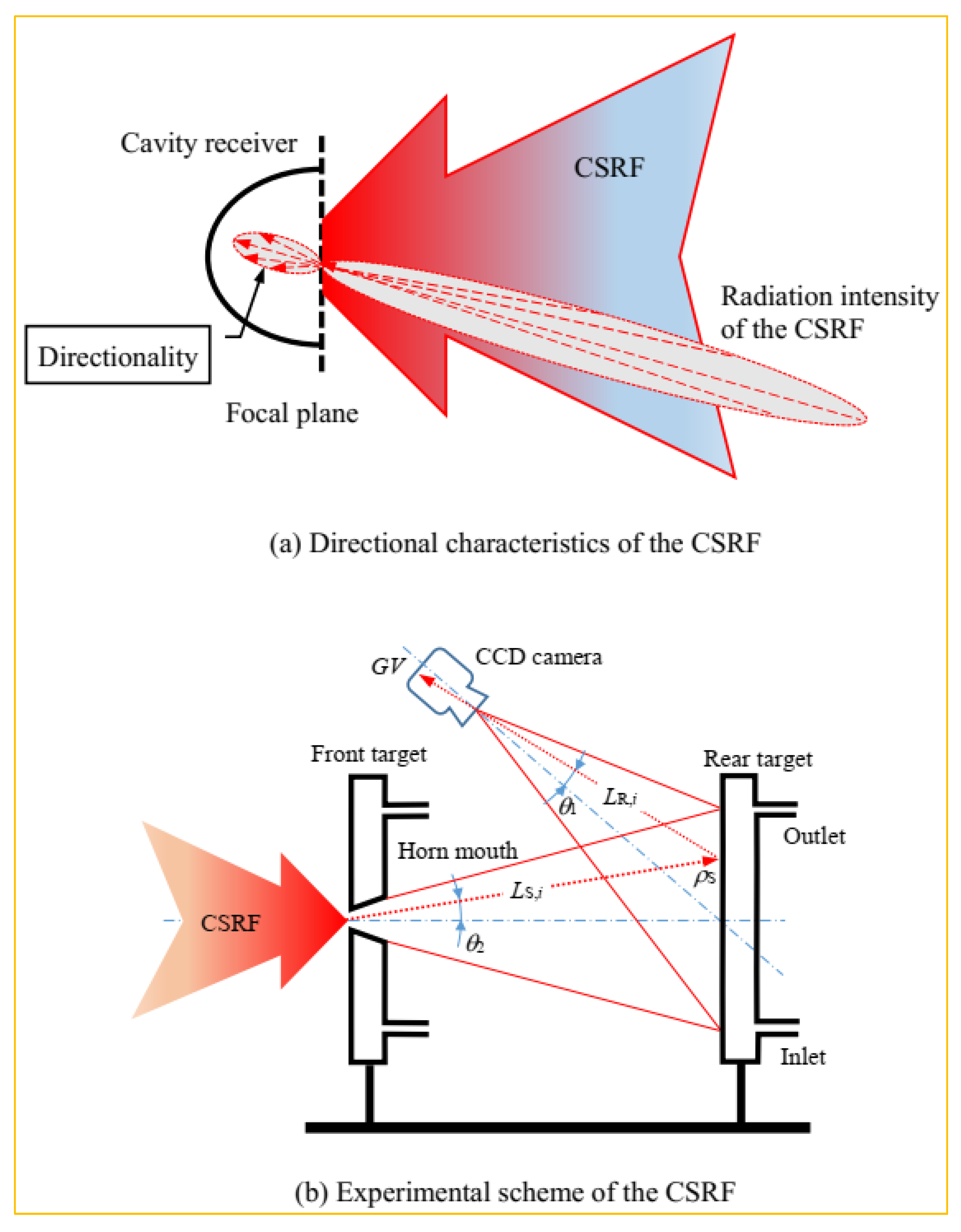
2.1. Experimental Method

The optical path for measuring the directional distributions of the CSRF is shown in Figure 1. Figure 1a shows the directional characteristics of the CSRF, where the spatial CSRF value is equal to the integration of the radiant intensity at the local position over the solid angle. As shown in Figure 1b, along the transmission direction of the incoming sunlight emitted from the solar simulator, both the front and the rear target (water-cooled) are installed on a three-dimensional movable platform. So, their relative positions are fixed during the experimental measurement.

The left side surface of the front target coincides with the focal plane of the solar simulator during the measurement. At the center point of the front target there is a small horn mouth, which enables local incoming sunlight to penetrate through the front target and illuminate the rear target. Then the CCD camera photographs the CSRF maps on the rear target. By adjusting the geometric positions of the three-dimensional movable platform, the CSRF maps at different positions of the focal plane can be measured and obtained through the image data analysis of the CCD camera.

Using a uniform light source and a luxmeter, the relationship between the gray value of the CCD camera and the radiative power can be expressed approximately as [16]:

$$L=a_{\mathrm{c}}\cdot GV+b_{\mathrm{c}}$$

(1)

In the above equation, the symbol L is the radiative power of the uniform light source, measured by the luxmeter, W/m². The symbol GV is the gray value of the CCD camera. The symbols a_c and b_c are the fitting coefficients of the CCD camera, respectively.

To describe the directional distribution characteristics of the CSRF, a coordinate system o-xyz is set up between the front and the rear target. The xoy plane is fixed on the left side surface of the front target and the original point is located at the center point of the horn mouth. The z coordinate points at the rear target. The left side surface of the rear target is divided into surface elements along the x axis and the y axis direction uniformly. For the convenience of analysis, the number of the surface elements is equal to the pixel number of the image. According to Equation (1), the incoming solar radiative power of the CSRF presented at surface element (i, j) can be calculated by the following formula:

$$L_{\mathrm{S},\left(i,j\right)}=\frac{a_{\mathrm{c}}\cdot G{V}_{\mathrm{S},\left(i,j\right)}+b_{\mathrm{c}}}{{\rho }_{\mathrm{S}}\cdot f_{\mathrm{S}}}$$

(2)

In Equation (2), the symbol $L_{\mathrm{S},\left(i,j\right)}$ is the incoming solar radiative power at surface element (i, j), W/m². The symbol ${\displaystyle {\rho }_{\mathrm{S}}}$ is the reflectivity of the left side surface of the rear target, and it is about 0.8. The symbol $f_{\mathrm{S}}$ is the transmittance of the neutral density filter installed at the CCD camera during the measurement. The symbol $G{V}_{\mathrm{S},\left(i,j\right)}$ is the gray value at pixel (i, j) of the image photographed by the CCD camera.

Both the zenith angle and the circumferential angle of the CSRF at surface element (i, j) can be estimated through the geometry relationships between the horn mouth and the left side surface of the rear target through the following expressions:

$${\theta }_{\left(i,j\right)}=\arctan \left(\frac{\sqrt{x_i^2+y_j^2}}{l}\right)$$

(3a)

$${\beta }_{\left(i,j\right)}=\{\begin{array}{l}\arccos \left(\frac{x_i}{\sqrt{x_i^2+y_j^2}}\right), y_j>0\\ 2\pi -\arccos \left(\frac{x_i}{\sqrt{x_i^2+y_j^2}}\right), y_j<0\end{array}$$

(3b)

In the above equations, the symbols ${\theta }_{\left(i,j\right)}$ and ${\beta }_{\left(i,j\right)}$ are the zenith angle and the circumferential angle of the CSRF at surface element (i, j). The symbol l is the spacing between left side surface of the front and the rear target, which is set to 200 mm, as shown in Figure 1b. The symbols $x_i$ and $y_j$ are the x coordinate and the y coordinate of surface element (i, j), which can be calculated by the following equation:

$$x_i=i\cdot \frac{h_x}{N_x}-\frac{h_x}{2}$$

(4a)

$$y_j=j\cdot \frac{h_y}{N_y}-\frac{h_y}{2}$$

(4b)

In the above equation, the symbols i and j are the order number of surface element (i, j) along the x axis and the y axis direction; the symbols $h_x$ and $h_y$ are the size of the rear target surface along the x axis and the y axis direction; the symbols $N_x$ and $N_y$ are the pixel numbers of the surface image.

The directional distributions of the concentrated solar radiative intensity (CSRI) and the relative CSRI are defined as follows:

$$I_{\mathrm{S}}=\frac{L_{\mathrm{S}}\cdot \Delta A}{\Delta \Omega \cdot \Delta A_{\mathrm{H}\mathrm{M}}\cdot \cos \theta }$$

(5)

$${I^{\prime }}_{\mathrm{S}}=\frac{I_{\mathrm{S}}}{I_{\mathrm{S},\max }}$$

(6)

where the symbols $I_{\mathrm{S}}$ and ${I^{\prime }}_{\mathrm{S}}$ are the CSRI and the relative CSRI receptivity. The symbol $L_{\mathrm{S},\max }$ is the maximal CSRI. The symbol $L_{\mathrm{S}}$ is defined in Equation (2). The symbol $\Delta A_{\mathrm{HM}}$ is the area of the horn mouth and $\theta$ is the zenith angle as defined in Equation (3a). The symbols $\Delta \mathsf{\Omega }$ and $\Delta A$ are the micro solid angle and the micro area of surface element (i, j) on the rear target. The micro solid angle $\Delta \mathsf{\Omega }$ can be expressed as:

$$\Delta \mathsf{\Omega }=\frac{\Delta A\cdot \cos \theta }{{\left(l/\cos \theta \right)}^2}=\frac{\Delta A\cdot {\cos }^3\theta }{l^2}$$

(7)

Substituting Equation (7) in Equation (5) gives:

$$I_{\mathrm{S}}=\frac{L_{\mathrm{S}}\cdot l^2}{{\cos }^4\theta }$$

(8)

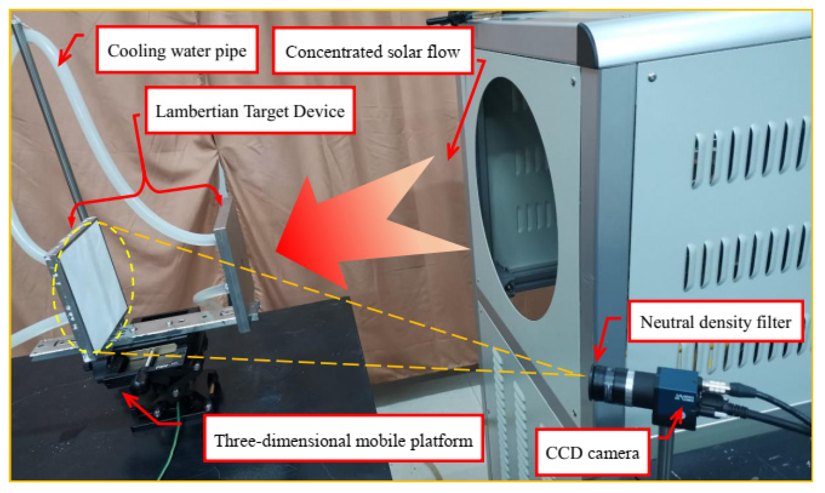
2.2. Experimental Apparatus

Figure 2 shows the experimental apparatus of the CSRF measurement, which mainly includes the water-cooled Lambertian target device (the front and the rear target), solar simulator, and the CCD camera fixed with the neutral density filter. According to the optical path in Figure 1, the beam emitted from the solar simulator penetrates the horn mouth of the front target and arrives at the left side surface of the rear target. Then, the beam image was shot using the CCD camera with the neutral density filter to form the gray image.

(1) The water-cooled Lambertian target device includes double Lambertian targets (front target and rear target), which are water-cooled to take away the radiation energy absorbed and reduce the temperature, as shown in Figure 3a. A horn mouth is set at the center point of the front target to ensure that all of the local incident sunlight can pass through it. To produce the Lambertian targets, both the left side surfaces of the front and rear target were covered with barium sulfate slurry until it was dry. Both the front and rear targets are made up of stainless-steel plates with an external size of 150 mm × 150 mm × 15 mm. To circulate the cooling water, the targets are hollow structures with a wall thickness of 5 mm, the right side surface of the front target is shown in Figure 3b. In repeated testing, the spacing between the two targets was set to 200 mm during measurement.

(2) The solar simulator mainly includes a xenon light source, an ellipsoidal concentrator, an air-cooling system, and a water-cooling system, etc. The maximum input power is 10 kW, the maximum radiant power is 3 kW (electro-optical conversion efficiency is about 30%, the spectral energy distribution is similar to atmospheric mass 1.5). The spot diameter is less than 80 mm, and the peak flux is less than 3 MW/m².

(3) The CCD camera is MER-201-25GM with a resolution of 1682 × 1236. During the measurement, the CCD camera was arranged with the lens pointed to the left side surface of the rear target. Through personal computer operation, the image of the sun spot on the rear target was captured and recorded.

(4) A neutral density filter is necessary to reduce the target radiative intensity and prevent saturation of the CCD camera. The transmittance of the neutral density filter generally includes 1%, 10%, 30%, 50%, etc. During both the calibration experiment and CSRF experiment, multiple neutral density filters should be set in series to ensure that the peak gray value of the image is about 200.

Before the experimental measurement of the CSRF map, the fitting coefficients of the CCD camera in Equation (1) should be determined. In this study, an integrating sphere source (with diameter of 30 cm and maximum power of 36 W) was used to calibrate the CCD camera. According to the calibration test, the value of the symbol a_c and b_c in Equation (1) are equal to 0.08778 and −0.6112, respectively.

In short, the experimental measurement and data processing procedure can be summarized as follows:

Firstly, turn on the cooling system, and then turn on the xenon light source. Adjust the Lambertian target position to ensure that the focal plane coincides with the front target surface.

Secondly, photograph the image of the CSRF on the left side surface of the rear target when the irradiation is stable. By adjusting the three-dimensional mobile platform, record the spot images of the CSRF at different points along the focal plane.

Thirdly, read out the gray value of the spot images by applying MATLAB software, and calculate the radiative intensity using Equation (2) for all of the surface elements.

Finally, calculate the tangential angle and the radial angle of surface element (i, j) through Equation (3). Combining the results from Equations (2) and (3), it is possible to measure the directional distributions of the CSRF at different points along the focal plane.

The total uncertainty of the experimental result is composed of type A and B uncertainty. Type A uncertainty is calculated using an error analysis method with the gray value of the spot images, and type B uncertainty is determined by the accuracy of the instrument. Therefore, the total uncertainty can be calculated using the following expression:

$$\mu =\sqrt{{\mu }_{\mathrm{A}}^2+{\mu }_{\mathrm{B}}^2}$$

(9)

In the above equation, the symbol ${\mu }_{\mathrm{A}}$ and ${\mu }_{\mathrm{B}}$ are type A and B uncertainty, respectively.

To calculate type A uncertainty, the spot image of the CSRF is measured repeatedly 20 times. The arithmetic mean value of the samples and the experimental standard deviation are calculated separately (the significance level of Grubbs criterion is taken as 5%). The symbol ${\mu }_{\mathrm{A}}$ is equal to 1.32% in this study. Type B uncertainty mainly includes the uncertainty of the diffuse reflection of the Lambertian target surface, the uncertainty of the neutral density filter and the uncertainty of the CCD camera, which are equal to 2.6%, 0.5% and 3.72%, respectively, through the analysis. Consequently, the total uncertainty is about 4.76% calculated by Equation (9), which satisfies the measurement demands.

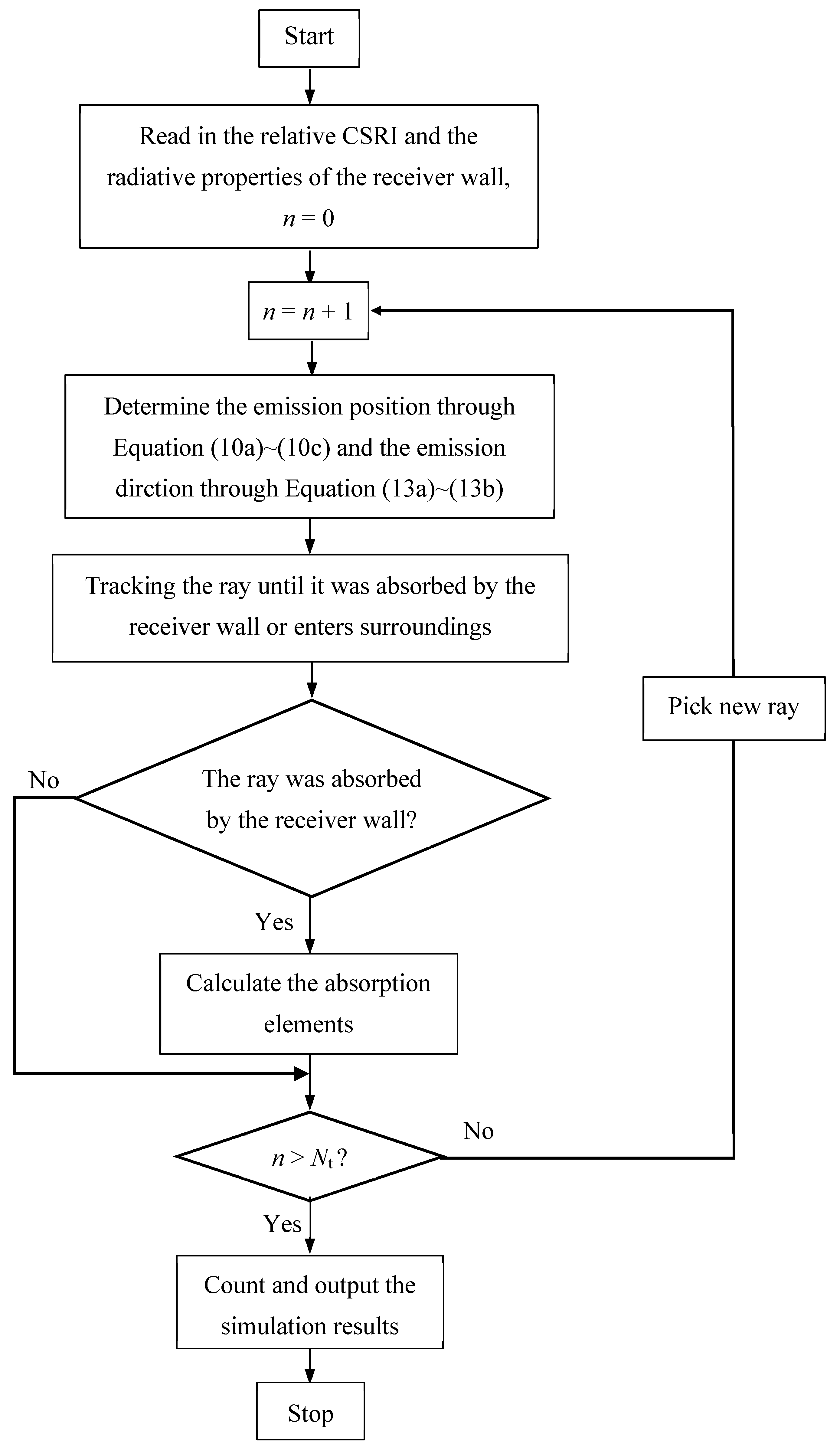
3. MCRTM Method Coupled with Experimental CSRF on the Focal Plane

For convenience of analysis, a hemisphere cavity receiver was taken as an example to illustrate the influences of the directional distributions of the CSRF on the solar concentrating characteristics, as shown in Figure 1a. Based on the experimental spatial and directional distributions of the CSRI on the focal plane, the wall flux images of the cavity receiver were simulated by applying the Monte Carlo ray-tracing method (MCRTM). MCRTM obtains the statistical results by tracking massive and independent solar rays from the emission position to the absorption position. The transmission process of each ray is composed of a series of independent sub-processes (emission, reflection, and absorption), and each independent sub-process follows a specific probability model [18].

On the focal plane, the probability function of the emission position for each solar ray is given by the following expression:

$$x_0=r\cdot \cos \left(2\pi \cdot R_{\phi }\right)$$

(10a)

$$y_0=r\cdot \sin \left(2\pi \cdot R_{\phi }\right)$$

(10b)

$$z_0=0$$

(10c)

In the above equation, the symbol $R_{\phi }$ is the random number which is uniformly distributed between zero and one. The symbol r is the emission radius for the solar ray given by:

$$R_r=\frac{{\displaystyle {\int }_0^r{q}_{\mathrm{s}}(r)\cdot 2\pi r^{\prime }\mathrm{d}{r}^{\prime }}}{{\displaystyle {\int }_0^{r_0}{q}_{\mathrm{s}}(r)\cdot 2\pi r^{\prime }\mathrm{d}{r}^{\prime }}}$$

(11)

where the symbol $R_r$ is the random number which is uniformly distributed between zero and one. $r_0$ is the maximal radius of the CSRF on the focal plane, and $r_0=0.04 \mathrm{m}$. The symbol $q_{\mathrm{s}}(r)$ is the spatial density distribution of the CSRF on the focal plane, as shown in Equation (14).

Inserting Equation (14) into Equation (11) and collecting the terms yields the expression of $r$ as:

$$r=\sqrt{-\frac{\ln \left(1-0.98336R_r\right)}{2560}}$$

(12)

The emission direction of the solar rays can be defined by the zenith angle $\theta$ and the circumferential angle $\beta$. The probability function of the zenith angle and the circumferential angle can be calculated using the discrete experimental data directly through the following form [17]:

$$R_{\beta }=\frac{{\displaystyle \sum _{{\beta }^{\prime }=0}^{\beta }{\displaystyle \sum _{{\theta }^{\prime }={\theta }_{\min }}^{{\theta }_{\max }}{I^{\prime }}_{\mathrm{S}}\cos {\theta }^{\prime }\sin {\theta }^{\prime }\mathrm{d}{\theta }^{\prime }\mathrm{d}{\beta }^{\prime }}}}{{\displaystyle \sum _{{\beta }^{\prime }=0}^{2\pi }{\displaystyle \sum _{{\theta }^{\prime }={\theta }_{\min }}^{{\theta }_{\max }}{I^{\prime }}_{\mathrm{S}}\cos {\theta }^{\prime }\sin {\theta }^{\prime }\mathrm{d}{\theta }^{\prime }\mathrm{d}{\beta }^{\prime }}}}$$

(13a)

$$R_{\theta }=\frac{{\displaystyle \sum _{{\theta }^{\prime }={\theta }_{\min }}^{\theta }{I^{\prime }}_{\mathrm{S}}\cos {\theta }^{\prime }\sin {\theta }^{\prime }\mathrm{d}{\theta }^{\prime }}}{{\displaystyle \sum _{{\theta }^{\prime }={\theta }_{\min }}^{{\theta }_{\max }}{I^{\prime }}_{\mathrm{S}}\cos {\theta }^{\prime }\sin {\theta }^{\prime }\mathrm{d}{\theta }^{\prime }\mathrm{d}{\varphi }^{\prime }}}$$

(13b)

where the symbols $R_{\beta }$ and $R_{\theta }$ are the random number, which is uniformly distributed between zero and one, respectively. The symbols ${\theta }_{\min }$ and ${\theta }_{\max }$ are the maximal and the minimal value of the zenith angle, respectively, and ${\theta }_{\min }=0.05 \mathrm{rad}$, ${\theta }_{\max }=0.25 \mathrm{rad}$ as discussed above. The symbol ${I^{\prime }}_{\mathrm{S}}$ is discrete experimental data of the relative CSRI.

To calculate the value of circumferential angle $\beta$ from Equation (13a), we should give the random number $R_{\beta }$ first. Then, accumulate the right side of Equation (13a) along the circumferential angle $\beta$ step by step. Once the accumulated value is larger than $R_{\beta }$, the current $\beta$ is just the solution. A similar calculation process is suitable to solve the zenith angle $\theta$ from Equation (13b). To ensure the convergence of the statistical results calculated by MCRTM (with a relative error less than 0.1%), 10⁹ solar rays were sampled for each case. The flowchart of the MCRTM together with the measured results is shown in Figure 4, where the emission positions and the directions are determined by the measured relative CSRI. The symbol N_t is the total ray number sampled, which is set to 10⁹ as discussed.

4. Measurement Results and Experimental Verification

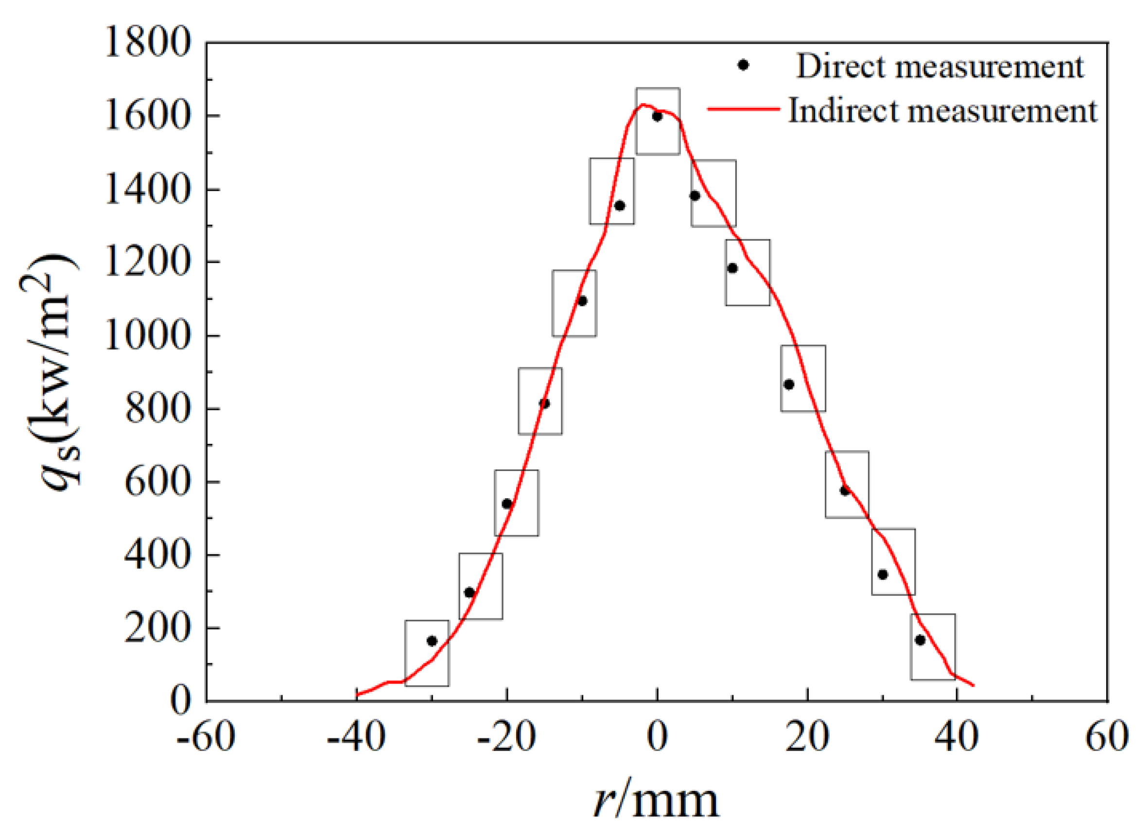
4.1. Composite Measurement of the CSRF Density Distributions

In order to verify the accuracy of the CCD measurement, a composite experimental method that comprises the direct and the indirect measurement was conducted to measure the spatial distribution of the CSRF on the focal plane. For the direct measurement, the probe of the heat flux meter (GD-B3-3M) was fixed on the focal plane. The CSRF values at different positions were tested by the heat flow meter through moving the three-dimensional mobile platform. Using this measurement, the heat flux values of thirteen positions uniformly along the vertical axis were recorded and obtained. The peak value around the center of the focal plane is up to 1601.5 kW/m², as shown in Figure 5.

Meanwhile, the CSRF spot was obtained through the indirect measurement, which was carried out using the CCD camera together with the rear target. To avoid the saturation of the CCD camera when exposed to the CSRF, four neutral density filters with identical transmissivity of 1% ware arranged in series ($f_{\mathrm{S}}={10}^{-8}$). Results show that the CSRF spot is asymmetric, and the effective diameter of the spot is about 60 mm. The peak value at the center of the spot is about 1655.4 kW/m². The relative error of the peak heat flux density between the direct and the indirect measurements is about 3.6%. Because the probe of the heat flux meter is too large compared to a single pixel on the curve, the value recorded by the heat flux meter represents the average gray value of the CCD graph inside the rectangular box.

Moreover, the spatial distribution of the CSRF spot on the focal plane can be fitted using the Gaussian function as follows:

$$q_{\mathrm{s}}(r)=A\exp (-B{r}^2)$$

(14)

where the symbol r is the radius of the CSRF spot, m. The symbols A and B are the fitting coefficients of the experimental curve, respectively. In this measurement, A = 1.655 × 10⁶ W/m², B = 2560 m⁻².

4.2. The Directional Characteristics of the CSRF

To measure the directional characteristics of the CSRF, the horn mouth of the front target was positioned at the center point O (0,0) of the focal plane. After the image of the CSRF spot on the rear target surface was stabilized, the CCD camera was used to shoot the gray value image (the transmissivity $f_{\mathrm{S}}$ of the neutral density filters was set to 10⁻⁵ to avoid the saturation of the CCD camera), as shown in Figure 6a.

Figure 6b shows the corresponding CSRF value computed by the gray value image through Equation (2). It can be seen clearly from Figure 6b that the CSRF image is uneven and spinous. Most heat fluxes are located in the first quadrant, and the peak value of the heat flux is about 1700 kW/m². In the other three quadrants, the CSRF distributions are relatively uniformly and low. There is a blue hole in the central region, which means that the heat flux in this region is negligible.

Figure 6c shows the CSRF image in the spherical coordinates, where the zenith angle and the circumferential angle are calculated through Equation (3a,b). It can be found that the directional distribution of the CSRF is non-uniform along the zenith angle and the circumferential angle. Most CSRF locates in the tangential angle only from 0.05 to 0.3 rad, in the other range there is no heat flux. Furthermore, the CSRF illuminate the entire circumferential angle ranges. In addition, the value of the CSRF in the first quadrant is evidently greater than that in the other quadrants.

For convenience of analysis, the directional distributions of the CSRF in Figure 6c can be fitted using the piecewise Gaussian functions along the zenith angle and the circumferential angle as follows:

$$q_{\mathrm{s}}(\theta ,\beta )=\{\begin{array}{c}-0.167+2.00\exp \left[-\frac{1}{2}{\left(\frac{\theta -0.14}{0.09}\right)}^2-\frac{1}{2}{\left(\frac{\beta -0.54}{0.93}\right)}^2\right],\beta =\left(0~0.51\right)\pi ,R=0.911\\ -0.046+1.18\exp \left[-\frac{1}{2}{\left(\frac{\theta -0.11}{0.08}\right)}^2-\frac{1}{2}{\left(\frac{\beta -1.99}{1.51}\right)}^2\right],\beta =\left(0.51~0.96\right)\pi ,R=0.912\\ -0.003+1.05\exp \left[-\frac{1}{2}{\left(\frac{\theta -0.13}{0.07}\right)}^2-\frac{1}{2}{\left(\frac{\beta -4.11}{2.25}\right)}^2\right],\beta =\left(0.96~1.66\right)\pi ,R=0.846\\ -0.160+1.34\exp \left[-\frac{1}{2}{\left(\frac{\theta -0.17}{0.09}\right)}^2-\frac{1}{2}{\left(\frac{\beta -6.19}{3.11}\right)}^2\right],\beta =\left(1.66~2.0\right)\pi ,R=0.85\end{array}$$

(15)

In the above equation, the symbol $q_{\mathrm{s}}(\theta ,\beta )$ is the directional distribution of the CSRF at the center point of the focal plane and the symbols $\theta$ and $\beta$ are the tangential angle and the radial angle, respectively. The symbol R denotes the correlation coefficient of the fitting functions. It can be found that all of the correlation coefficients of the fitting functions in Equation (15) are larger than 0.84, which means the fitting functions are quite reliable.

Figure 6d shows the directional distributions of the relative CSRI (as defined in Equation (6)) in the spherical coordinates. It can be found that the profile of the relative CSRI image is similar to that of the CSRF image in Figure 6c because the tangential angle range is rather small and its cosine values approach 1.0.

From the experimental measurement, it can be also found that the directional distributions of the CSRF of the other points on the focal plane are similar to that of the center point O, where the relative CSRI is also the Gaussian distribution over a certain solid angle range.

4.3. Influences of the Directional CSRI on Thermal Conditions of the Cavity Receiver

Figure 7 shows the CSRF images on the wall of the hemisphere cavity receiver with a radius of 0.05 m under two directional CSRF distributions on the focal plane. Figure 7c shows the CSRF images in the case of the uniform directional CSRI with the zenith angle from 0.0 to 0.3 rad. Figure 7b shows the CSRF images in the case of the measured directional CSRI plotted in Figure 6d. For comparison, the wall emissivity of the hemisphere cavity is given as 0.85 for both cases, and the spatial distribution of the CSRF on the focal plane are also identical as presented in Equation (14).

It can be found from Figure 7a that the CSRF image is Gaussian shape in spherical coordinates, where the CSRF value decreases with the increasing of the zenith angle, and the peak value appears at the top of the hemisphere cavity. The CSRF value becomes rather uniform along the circumferential angle. However, the CSRF image in Figure 7b is asymmetric round the symmetry axis of the hemisphere cavity receiver due to the complexity of the measured directional CSRI distributions, where the concentrated solar energy in the first quadrant is more than that in the other two quadrants. In general, the CSRF images of the cavity receiver depend on both the spatial CSRF and the directional CSRI of the focal plane. When the geometry size of the cavity receiver is small, the CSRF images of the cavity receiver are dominated by the spatial CSRF of the focal plane because the transmission distance of the CSRF is short and the influence of the directional CSRI is limited. However, the influence of the directional CSRI will be amplified with increasing geometry size of the hemisphere cavity. The transmission distances of the CSRF will dominate the CSRF images of the cavity receiver, and the peak CSRF element of the cavity receiver always occurs at the orientation of the maximum CSRI.

Figure 7c shows the difference image between the CSRF in Figure 7b and that in Figure 7a. It can be seen that there is a bright spot in the right side of the hemisphere cavity receiver, and the differential value ranges from −0.16 MW/m² to 0.1 MW/m². The relative error of the CSRF value in Figure 7b and that in Figure 7c is up to 16%. These values prove that the directional CSRI plays an important role in the CSRF images of the cavity receiver. More accurate thermal conditions of solar receivers can be obtained when both the spatial CSRF and the directional CSRI are measured together. It is beneficial to the heat transfer improvement of solar thermal applications.

5. Conclusions

In this paper, double water-cooled Lambertian targets were developed to measure the spatial and directional distributions of the CSRF at the focal plane emitted from the sun simulator. The uncertainty of the experimental data is about 4.76% according to error analysis. The directional distributions of the CSRF are spinous and the piecewise Gaussian function should be used to fit the measured data. The CSRF images on the cavity wall in the case of the spinous CSRF were quite different from those of the uniform directional CSRF. The relative error of the peak CSRF images between two cases was up to 16%. Clearly, it is essential to measure the vectorial CSRF distribution on the focal plane because we are capable of predicting more accurate thermal conditions of the solar receiver.

It also necessary to note that this measurement method of the vectorial CSRF was performed by applying a solar simulator and the experimental data is steady. However, the experimental process and the data would be unsteady for the solar concentrators. In addition, multiple neutral density filters are needed to ensure that the peak value of the image is about 200 for both the calibration experiment and the CSRF experiment.

References

1. Ávila-Marín, A.L. Volumetric receivers in solar thermal power plants with central receiver system technology: A review. Sol. Energy 2011, 85, 891–910. [Google Scholar] [CrossRef]
2. Avila-Marin, A.L.; Fernandez-Reche, J.; Martinez-Tarifa, A. Modelling strategies for porous structures as solar receivers in central receiver systems: A review. Renew. Sustain. Energy Rev. 2019, 111, 15–33. [Google Scholar] [CrossRef]
3. Cagnoli, M.; Froio, A.; Savoldi, L.; Zanino, R. Multi-scale modular analysis of open volumetric receivers for central tower CSP systems. Sol. Energy 2019, 190, 195–211. [Google Scholar] [CrossRef]
4. Patil, V.R.; Kiener, F.; Grylka, A.; Steinfeld, A. Experimental testing of a solar air cavity-receiver with reticulated porous ceramic absorbers for thermal processing at above 1000 °C. Sol. Energy 2021, 214, 72–85. [Google Scholar] [CrossRef]
5. Ballestrin, J. A non-water-cooled heat flux measurement system under concentrated solar radiation conditions. Sol. Energy 2002, 73, 159–168. [Google Scholar] [CrossRef]
6. Röger, M.; Herrmann, P.; Ulmer, S.; Ebert, M.; Prahl, C.; Göhring, F. Techniques to Measure Solar Flux Density Distribution on Large-Scale Receivers. J. Sol. Energy Eng. 2014, 136, 031013–1–031013–10. [Google Scholar] [CrossRef] [Green Version]
7. Wang, Y.; Liu, Q.; Lei, J.; Liu, F. Design and characterization of the non-uniform solar flux distribution measurement system. Appl. Therm. Eng. 2019, 150, 294–304. [Google Scholar] [CrossRef]
8. Ulmer, S.; Lüpfert, E.; Pfänder, M.; Buck, R. Calibration corrections of solar tower flux density measurements. Energy 2004, 29, 925–933. [Google Scholar] [CrossRef]
9. Krueger, K.R.; Lipinski, W.; Davidson, J.H. Operational performance of the university of minnesota 45 kWe High-Flux Solar Simulator. J. Sol. Energy Eng. 2013, 135, 044501.1–044501.4. [Google Scholar] [CrossRef]
10. Li, J.; Gonzalez-Aguilar, J.; Pérez-Rábago, C.; Zeaiter, H.; Romero, M. Optical analysis of a hexagonal 42kWe high-flux solar simulator. Energy Procedia 2014, 57, 590–596. [Google Scholar] [CrossRef]
11. Sarwar, J.; Georgakis, G.; LaChance, R.; Ozalp, N. Description and characterization of an adjustable flux solar simulator for solar thermal, thermochemical and photovoltaic applications. Sol. Energy 2014, 100, 179–194. [Google Scholar] [CrossRef]
12. Levêque, G.; Bader, R.; Lipiński, W.; Haussener, S. Experimental and numerical characterization of a new 45 kWel multisource high-flux solar simulator. Opt. Express 2016, 24, A1360–A1373. [Google Scholar] [CrossRef] [PubMed]
13. Aichmayer, L.; Wang, W.; Garrido, J.; Laumert, B. Experimental flux measurement of a high-flux solar simulator using a Lambertian target and a thermopile flux sensor. In AIP Conference Proceedings; AIP Publishing LLC: Melville, NY, USA, 2016. [Google Scholar]
14. Ballestrín, J.; Monterreal, R. Hybrid heat flux measurement system for solar central receiver evaluation. Energy 2004, 29, 915–924. [Google Scholar] [CrossRef]
15. Xiao, J.; Wei, X.; Gilaber, R.N.; Zhang, Y.; Li, Z. Design and characterization of a high-flux non-coaxial concentrating solar simulator. Appl. Therm. Eng. 2018, 145, 201–211. [Google Scholar] [CrossRef]
16. Xiao, J.; Yang, H.; Wei, X.; Li, Z. A novel flux mapping system for high-flux solar simulators based on the indirect method. Sol. Energy 2019, 179, 89–98. [Google Scholar] [CrossRef]
17. Modest, M. Radiative Heat Transfer; Academic Press: Cambridge, MA, USA, 2003. [Google Scholar]
18. Shuai, Y.; Xia, X.L.; Tan, H.P. Radiation performance of dish solar concentrator/cavity receiver systems. Sol. Energy 2008, 82, 13–21. [Google Scholar] [CrossRef]
19. Chen, X.; Xia, X.L.; Liu, H.; Li, Y.; Liu, B. Heat transfer analysis of a volumetric solar receiver by coupling the solar radiation transport and internal heat transfer. Energy Convers. Manag. 2016, 114, 20–27. [Google Scholar] [CrossRef]
20. Ali, M.; Rady, M.; Attia, M.A.; Ewais, E.M. Consistent coupled optical and thermal analysis of volumetric solar receivers with honeycomb absorbers. Renew. Energy 2020, 145, 1849–1861. [Google Scholar] [CrossRef]
21. Garcia, P.; Ferriere, A.; Bezian, J.J. Codes for solar flux calculation dedicated to central receiver system applications—A comparative review. Sol. Energy 2008, 82, 189–197. [Google Scholar] [CrossRef] [Green Version]
22. He, Y.L.; Cui, F.Q.; Cheng, Z.D.; Li, Z.Y.; Tao, W.Q. Numerical simulation of solar radiation transmission process for the solar tower power plant_ From the heliostat field to the pressurized volumetric receiver. Appl. Therm. Eng. 2013, 61, 583–595. [Google Scholar] [CrossRef]
23. Daabo, A.M.; Mahmoud, S.; Al-Dadah, R.K. The optical efficiency of three different geometries of a small scale cavity receiver for concentrated solar applications. Appl. Energy 2016, 179, 1081–1096. [Google Scholar] [CrossRef] [Green Version]
24. Daabo, A.M.; Ahmad, A.; Mahmoud, S.; Al-Dadah, R.K. Parametric analysis of small scale cavity receiver with optimum shape for solar powered closed Brayton cycle applications. Appl. Therm. Eng. 2011, 31, 3377–3386. [Google Scholar] [CrossRef]
25. Kasaeian, A.; Kouravand, A.; Rad, M.A.V.; Maniee, S.; Pourfayaz, F. Cavity receivers in solar dish collectors: A geometric overview. Renew. Energy 2021, 169, 53–79. [Google Scholar] [CrossRef]
26. Du, S.; He, Y.L.; Yang, W.W.; Liu, Z.B. Optimization method for the porous volumetric solar receiver coupling genetic algorithm and heat transfer analysis. Int. J. Heat Mass Transf. 2018, 122, 383–390. [Google Scholar] [CrossRef]
27. Barreto, G.; Canhoto, P.; Collares-Pereira, M. Three-dimensional CFD modelling and thermal performance analysis of porous volumetric receivers coupled to solar concentration systems. Appl. Energy 2019, 252, 113433. [Google Scholar] [CrossRef]
28. Kribus, A. Optical performance of conical windows for concentrated solar radiation. J. Sol. Energy Eng. 1994, 116, 47–52. [Google Scholar] [CrossRef]
29. Karni, J.; Kribus, A.; Ostraich, B.; Kochavi, E. A high-pressure window for volumetric solar receivers. J. Sol. Energy Eng. 1998, 120, 101–107. [Google Scholar] [CrossRef]
30. Timinger, A.; Spirkl, W.; Kribus, A.; Ries, H. Optimized secondary concentrators for a partitioned central receiver system. Sol. Energy 2000, 69, 153–162. [Google Scholar] [CrossRef]
31. Xia, X.L.; Dai, G.L.; Shuai, Y. Experimental and numerical investigation on solar concentrating characteristics of a sixteen-dish concentrator. Int. J. Hydrogen Energy 2012, 37, 18694–18703. [Google Scholar] [CrossRef]
32. Wang, K.; He, Y.L.; Qiu, Y.; Zhang, Y. A novel integrated simulation approach couples MCRT and Gebhart methods to simulate solar radiation transfer in a solar power tower system with a cavity receiver. Renew. Energy 2016, 89, 93–107. [Google Scholar] [CrossRef]
Figure 1. Optical path for the directional distribution measurement of the CSRF.
Energies 16 00136 g001
Figure 2. Experiment apparatus of the CSRF measurement.
Energies 16 00136 g002
Figure 3. Water-cooled Lambertian targets.
Energies 16 00136 g003
Figure 4. Flowchart of the MCRTM together with the measured results.
Energies 16 00136 g004
Figure 5. Composite measurement curves of the CSRF spot.
Energies 16 00136 g005
Figure 6. Direction distribution characteristics of the center point O (0,0) on the focal plane.
Energies 16 00136 g006
Figure 7. CSRF images on the hemisphere cavity wall with the wall emissivity of 0.85.
Energies 16 00136 g007
Disclaimer/Publisher’s Note: The statements, opinions and data contained in all publications are solely those of the individual author(s) and contributor(s) and not of MDPI and/or the editor(s). MDPI and/or the editor(s) disclaim responsibility for any injury to people or property resulting from any ideas, methods, instructions or products referred to in the content.